Óbuda University

(1)

Óbuda University

PhD Thesis

Multi-Directional Image Projections with Fixed Resolution for Object Recognition and Matching

Gábor Kertész

Supervisors:

Dr. Zoltán Vámossy Dr. habil. Sándor Szénási

Doctoral School of Applied Informatics and Applied Mathematics

Budapest, 2019.

(2)

Final Examination Committee:

Chair:

Prof. Dr. Péter Nagy, DSc Members:

Dr. Kálmán Palágyi, PhD (University of Szeged) Dr. Szabolcs Sergyán, PhD

Dr. László Csink, PhD

Full Committee of Public Defense:

Opponents:

Dr. Kálmán Palágyi, PhD (University of Szeged) Dr. László Csink, PhD

Chair:

Prof. Dr. Péter Nagy, DSc Secretary:

Dr. Edit Tóthné Laufer, PhD Replacement secretary / member:

Dr. József Tick, PhD Members:

Dr. Szilveszter Kovács, PhD (University of Miskolc) Dr. Szilveszter Pletl, PhD (University of Szeged)

Replacement member:

Dr. Ferdinánd Filip, PhD (J. Selye University) Date of Public Defense:

October 17th, 2019

(3)

Declaration

I, the undersigned,Gábor Kertész, hereby state and declare that this Ph.D. thesis represents my own work and is the result of my own original research. I only used the sources listed in the references. All parts taken from other works, either as word for word citation or rewritten keeping the original meaning, have been unambiguously marked, and reference to the source was included.

Nyilatkozat

AlulírottKertész Gáborkijelentem, hogy ez a doktori értekezés a saját munkámat mutatja be, és a saját eredeti kutatásom eredménye. Csak a hivatkozásokban fel- sorolt forrásokat használtam fel, minden más munkából származó rész, a szó szerinti, vagy az eredeti jelentést megtartó átiratok egyértelműen jelölve, és forráshivatkozva lettek.

Gábor Kertész

(4)

Acknowledgments

First of all, I would like to thank my doctoral supervisors,Dr. Zoltán Vámossy and Dr. habil. Sándor Szénási for their valuable, ongoing support during my doctoral studies. As a result of their professional leadership and the many years of their ded- icated work I became the researcher and lecturer that I am today. I am immensely grateful for the guidance and encouragement they have given me along this path.

I am thankful to the members of the committee, especiallyProf. Dr. Péter Nagy, Dr. Kálmán Palágyi,Dr. László Csink, andDr. Adrienn Dineva, for sacrificing time and providing feedback during the review of the dissertation.

Special thanks to the staff of the John von Neumann Faculty of Informatics; in particular Prof. Dr. Dezső Sima, Dr. habil. András Molnár, Dr. habil. Imre Felde and Dr. Szabolcs Sergyán for providing professional background and an inspiring environment. Thanks to my colleagueDániel Kiss for his regular professional help.

Thanks to the Doctoral School of Applied Informatics and Applied Mathematics, especially Prof. Dr. Aurél Galántaiand Prof. Dr. László Horváth for providing regular professional feedback and the opportunity to attend international conferences.

I am grateful to my colleagues at MTA SZTAKI for their patience when I finalized the dissertation.

I am thankful toDr. Éva Nagyné HajnalandDr. Márta Seebauer, for considering me capable, and starting me on this path.

I would like to thank my family, especially my parents, for their support and encouragement in helping me achieve my goals throughout my life. Without their selfless financial and spiritual support, my dissertation would not have been possible.

Thank you for the patience of my friends during the writing of the dissertation.

Balázs, Csaba, István and Zsolt provided much useful advice during our professional discussions. Thank you for the inspiration.

I am grateful to my current and former students for their hard work, which resulted in presented and awarded studies at the National Scientific Students’ Asso- ciations Conference.

I am grateful to János, who, many years ago, directed me to the teaching pro- fession – a turning point in my life.

Finally, I owe special thanks to Gina – this dissertation would not have been completed without her understanding, patience, and support.

(7)

Köszönetnyilvánítás

Szeretnék köszönetet mondani doktori témavezetőimnek, Dr. Vámossy Zoltánnak ésDr. habil. Szénási Sándornak a tanulmányaim során nyújtott folyamatos, értékes segítségükért. Szakmai vezetésük, több éves áldozatos tevékenységük eredményeként váltam azzá a kutatóvá és oktatóvá, aki ma vagyok. Mérhetetlenül hálás vagyok az iránymutatásért és ösztönzésért, amellyel végigsegítettek ezen az úton.

Köszönöm a bizottság tagjainak, kiemeltenProf. Dr. Nagy Péternek,Dr. Palágyi Kálmánnak,Dr. Csink Lászlónak ésDr. Dineva Adrienn-nek hogy idejüket áldozták és tanácsokkal láttak el a disszertáció áttekintése során.

Külön köszönettel tartozom munkatársaimnak az Óbudai Egyetem Neumann János Informatikai Karán, elsősorban Prof. Dr. Sima Dezsőnek, Dr. habil. Molnár Andrásnak, Dr. habil. Felde Imrének és Dr. Sergyán Szabolcsnak köszönöm a pro- fesszionális szakmai háttér biztosítását és az inspiráló környezetet. Köszönöm Kiss Dánielkollégámnak a rendszeres szakmai segítséget.

Köszönet az Alkalmazott Informatikai és Matematikai Doktori Iskolának, kü- lönösen Prof. Dr. Galántai Aurélnak és Prof. Dr. Horváth Lászlónak a rendszeres szakmai visszajelzést és a nemzetközi konferenciákon való részvételi lehetőség bizto- sítását.

Hálás vagyok az MTA SZTAKInál dolgozó kollégáimnak a türelmükért, amelyet a disszertáció befejezésekor tanúsítottak.

Köszönöm Dr. Nagyné Hajnal Évának és Dr. Seebauer Mártának, hogy évekkel ezelőtt rátermettnek tartottak, és elindítottak ezen az úton.

Köszönettel tartozom családomnak, elsősorban a szüleimnek a támogatásukért és ösztönzésükért, amellyel egész életemben segítettek a céljaim elérésében. Önzetlen anyagi és lelki támogatásuk nélkül a dolgozatom nem jöhetett volna létre. Köszönöm barátaim türelmét, amelyet a disszertáció megírása során tanúsítottak.

Számtalan hasznos tanáccsal látott el szakmai diszkusszióink soránBalázs,Csaba, Istvánés Zsolt, köszönöm az inspirációt.

Hálás vagyok a jelenlegi és egykori hallgatóimnak a lelkiismeretes munkájukért, melynek eredményeképp Tudományos Diákköri Konferencián bemutatott és díjazott pályamunkák, valamint közös publikációk születtek.

Hálával tartozomJánosnak, aki hosszú évekkel ezelőtt az oktatói pályára terelt, amely fordulópont volt az életemben.

Végül különleges köszönettel tartozom Ginának – ez a disszertáció nem készült volna el megértése, türelme és támogatása nélkül.

(8)

Multi-Directional Image Projections with Fixed Resolution for Object Recognition and Matching

Gábor Kertész

Abstract

The use of computer vision and image processing in traffic analysis and control has shown significant growth in recent years. In addition to traditional solutions (such as traffic counting, accident detection), multi-camera applications based on vehicle identification and tracking have also emerged.

Innovation is supported by the explosive growth of image classification efficiency in recent years, which is the result of machine learning, in particular, the rise of deep learning.

This dissertation introduces solutions for multi-camera vehicle tracking to recog- nize and match vehicles through multiple with low-resolution, low-quality camera images.

The first group of theses deal with multi-directional image projections. I have developed a method for mapping two-dimensional image functions to one-dimensional projection vectors similar to the Radon transformation. The novelty of the solution is the fixed bin number, which is independent of the projection angle and specified as the input to the procedure. The memory cost of the resulting projection matrix is independent of the size of the input image.

I have designed and implemented a parallel version of the method in a GPU environment, taking into account the specific architecture and properties of the graphics processors. Runtime is linear and speedup is proportional to the number of available processing units.

I have compared the defined multi-directional image projection method with lower dimensional procedures in case of object matching. After evaluating the results, I have found that by applying the method, accuracy increased significantly and by using a fixed number of bins, the efficiency improved as well.

In the second group of theses, I present my results related to object matching based on machine learning solutions. In accordance with the state-of-the-art solutions, I have designed a method based on a Siamese convolutional neural network, which is capable of handling image projections as input. For a comprehensive measurement, it was first necessary to review possible network architectures and develop a method that generates multiple Convolutional neural network architectures based on input matrix dimensions. Based on the known convolutional design patterns, I have developed an optimization method based on backtracking search for Neural Architecture Generation. Based on the given input size and the number of hidden layers, the algorithm makes suggestions for the architecture of the head parts of the Siamese structured neural network, having the memory cost of the parameters taken into account.

The resulting architectures can be trained in parallel on a cluster of multiple workstations with GPUs. For the implementation, I designed and implemented a Master/Worker method, where the scheduler optimizes parallel efficiency based on

(9)

the parameters of the architectures. Based on the measurement results, I found that the acceleration is approximately equal to the number of workstations involved.

During the investigations, I analyzed the effects of the application of different projection methods as input to the Siamese networks and compared the results to the classic image input based comparators. When evaluating the results, I concluded that the projection methods are suitable for object matching and the method based on the fixed number of bins is Pareto optimal in terms of pairing efficiency and memory cost.

(10)

Többirányú, rögzített felbontású képi vetületek objektumok felismerésére és párosítására

Kertész Gábor

Kivonat

A gépi látás és képfeldolgozás használata a forgalomelemzés és -irányítás terü- letén az elmúlt években jelentős növekedésnek indult. A hagyományos megoldások (például forgalomszámlálás, balesetészlelés) mellett a járművek azonosításán és kö- vetésén alapuló több-kamerás alkalmazások is megjelentek.

Az innovációt támogatja a képi klasszifikáció hatékonyságának elmúlt években tapasztalt robbanásszerű növekedése, amely a gépi tanulás, azon belül is a mélyta- nulás megjelenésének eredménye.

Jelen disszertáció több-kamerás járműkövetés témakörében mutat be megoldá- sokat a gépjárművek azonosítására és több képen keresztüli párosítására alacsony felbontású, gyenge minőségű kameraképek esetén.

Az első téziscsoport a többirányú képi vetületek témakörével foglalkozik. Kidol- goztam egy módszert, amely a Radon transzformációhoz hasonlóan alkalmas két- dimenziós képi függvények egydimenziós vetületi vektorokra való leképezésére. A megoldás újdonsága a vetületi szögtől független fix rekesszám, amely az eljárás be- meneteként megadható. Az így készített vetületi mátrix memóriaköltsége független a bemeneti kép méretétől.

Megterveztem és implementáltam a módszer párhuzamos változatát GPU környe- zetben, figyelembe véve a grafikus processzorok sajátos felépítését és tulajdonságait.

A futásidő lineáris, a gyorsulás az elérhető műveletvégzők számával arányos.

A kidolgozott többirányú képi vetületi módszert összevetettem alacsonyabb di- menziójú eljárásokkal egyezésvizsgálat esetén. Az eredmények kiértékelése után meg- állapítottam hogy a módszer alkalmazásával jelentősen nőtt a pontosság, illetve a fix rekesszámnak köszönhetően a hatékonyság is is javult.

A második téziscsoportban az egyezésvizsgálat gépi tanuláson alapuló megoldásá- val kapcsolatos eredményeim mutatom be. A korszerű megoldásoknak megfelelően, egy sziámi konvolúciós neurális hálózatra épülő módszert terveztem, amely alkalmas akár képi vetületet bemeneteként fogadni. Az átfogó méréshez elöször szükséges volt áttekinteni a lehetséges hálózati architektúrákat, és kidolgozni egy módszert amely többféle konvolúciós neurális hálózati architektúrát generál a bemeneti mátrix di- menzióihoz igazodva. Az ismert konvolúciós tervezési minták alapján kidolgoztam egy visszalépéses keresésen alapuló optimalizációs módszert neurális architektúra ge- nerálásra. Az algoritmus az adott bemeneti méret és a rejtett rétegek száma alapján tesz javaslatokat a sziámi szerkezetű neurális hálózat fej-részeinek architektúrájára, figyelembe véve a paraméterek memória-költségét.

Az így előállított architektúrák tanítása párhuzamosan is történhet, több, GPU- val felszerelt munkaállomásból álló klaszterben. A megvalósításhoz egy Master/

Worker elvű módszert terveztem és valósítottam meg, ahol az ütemező az archi- tektúrák paraméterei alapján optimalizálja a párhuzamos hatékonyságot. A mérési eredmények alapján megállapítottam hogy a gyorsítás megközelítőleg egyezik a be- vont munkaállomások számával.

(11)

A vizsgálatok során különféle vetületi módszerek alkalmazásának hatásait vizs- gáltam a sziámi hálózatok bemeneteként, és az eredményeket összehasonlítottam a hagyományos képi bemenetű komparátorokra. Az eredmények kiértékelésekor meg- állapítottam, hogy a vetületi módszerek alkalmasak objektum párosításra, valamint a fix rekesszámú módszer Pareto optimális a párosítás hatékonysága és memória költsége szempontjából.

(12)

Abbreviations & notations

In this study the following notations and abbreviations were used:

Abbrevations

PCC Pearson Correlation Coefficient CNN Convolutional Neural Network SNN Siamese Neural Network GPU Graphical Processing Unit FCN Fully Convolutional Network FC Fully Connected (layers)

MDIPFL Multi-directional Image Projections with Fixed Length LPT Longest Processing Times

Projections

I image matrix

I_i,j pixel value of image on coordinate (i, j)

N×M matrix size

π_H,π_V,π_D,π_A horizontal, vertical, diagonal, antidiagonal projection vectors S₂,S₄ two- and four-dimensional projection-based signatures

σ standard deviation

cov(·,·) covariance between two vectors

ρ_H, ρ_V, ρ_D, ρ_A correlation coefficient of horizontal, vertical, diagonal vectors r(·) rectified value of scalar

µ similarity

f(p, φ) =ˇ Rf Radon transform of function f

p line of summarization

α,φ rotational angle

LL,HL projection segments around point P

S number of bins

res resolution

start,end position of projection on segment LL+HL P⁺_H set of ρ_H correlation coefficients for true pairs P⁻_H set of ρ_H correlation coefficients for false pairs

(13)

Neural networks

O_W, O_H width and height of output IW, IH width and height of input F_W, F_H width and height of filter P_W, P_H horizontal and vertical padding S_W, S_H horizontal and vertical stride F_num number of filters

F_num⁽ⁱ⁾ number of filters in layeri

L_num number of convolutional and pooling layer pairs N_num number of neurons

Nnum⁽ⁱ⁾ number of neurons in layer i x∈X observations

c∈C categories

f(x) =c mapping of observations to categories S(·,·) predicted similarity of inputs

m∈M models

f_err(·) error rate of model

f_memory(·) parameter number of model m₁ m₂ m₁ Pareto dominates m₂

(14)

List of Figures

1.1 Horizontal (a) and vertical (b) image projections are calculated by summarizing the row and column values in the matrix. . . 7 1.2 Diagonal (a) and antidiagonal (b) image projections of a squared

image matrix. . . 7 1.3 The visualized projection signature of a vehicle observation. Subfigure

(a) shows the squared image of a rear-viewed vehicle. In diagrams (b), (c), (d) and (e), the horizontal, vertical, diagonal and antidiagonal projections are visualized (π_H, π_V, π_D and π_A, respectively). . . 8 2.1 The Shepp-Logan [54] phantom is a standard test image used in the

testing of image reconstruction algorithms: it consists of 10 differently sized, rotated ellipses with different intensity levels inside the squared area. . . 14 2.2 The transformation of the sinus wave is formalized as Asin(α+β),

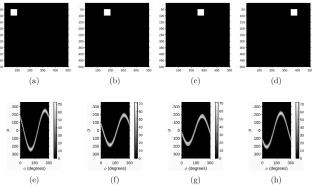
where A stands for the amplitude and β is the phase shift. . . 15 2.3 The results of horizontal translation on the sinogram: subfigures (a),

(b), (c) and (d) show the input image, where the object is shifted to the right. Subfigures (e), (f), (g) and (h) present the sinograms for each input image [K2]. It is notable, that the changes of the amplitude are directly affected by the distance changes from the center of the image. . . 16 2.4 The effect of shifting in Radon space results in rotation. The original

image (in subfigure (a)), and the sinogram of its projection sums (in subfigure (e)). To illustrate the effect of the circular shifting, the resulting matrix of the Radon transform is shifted byφ=π/2,π and π/6, presented in subfigures (b), (c) and (d), respectively. Subfigures (f), (g) and (h) show the result of the reconstruction after shifting [K2]. 17 2.5 Insignificant regions in the sinogram. In subfigure (a) is the image

representation of the matrix defined in (2.14). In subfigure (b) is the sinogram of the Radon transform of the image. The regions above and below the projection of the corner points are insignificant [K2]. . 18 2.6 The Radon transform of a unit matrix. In subfigure (a) is the image

representation of the unit matrix defined in (2.15). Subfigure (b) shows the sinogram of the Radon transform of this image. Note, that the intensity is affected by the number of pixels summarized: the brightest points are in the centers of the diagonal and antidiagonal projections at 45, 135, 225 and 315 degrees [K2]. . . 18

(15)

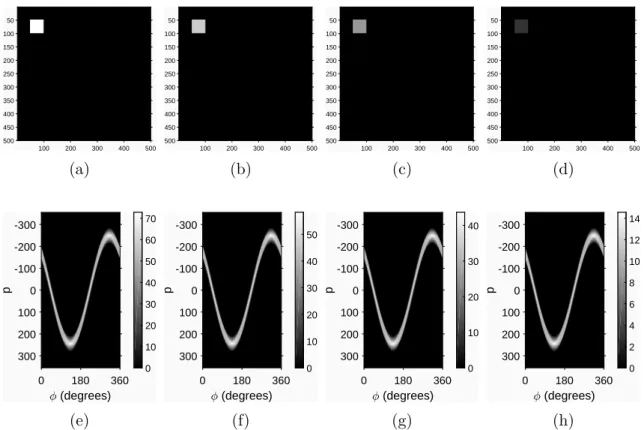
2.7 The effect of intensity changes on the sinogram. Subfigures (a), (b), (c) and (d) show the input image, where the object intensity is 1, 0.8, 0.6 and 0.2, respectively, and subfigures (e), (f), (g) and (h) presents the sinograms for the input images [K2].

While the forms of the sinusoids are the same, the intensity levels (visible on the bars) are different. . . 19 2.8 The effect of noise in the Radon space. Subfigure (a) shows the origi-

nal image with a zero mean, 0.1 variance Gaussian noise. In (b), the sinogram of the original image is visualized. In (c) is the Gauss filtered original image. Subfigure (d) gives the reconstructed image. Note, that the reconstruction removes some noise. Subfigure (e) shows the sinogram after filtering each column with a moving average filter, and in subfigure (f) is the reconstructed image of this method [K2]. . . 20 2.9 A sample vehicle image in subfigure (a) and the sinogram of the

Radon transform for the same image for angles [0; 2π) in subfigure (b). . . 22 2.10 (a) The proposed method with fixed bin sizes. Rotational angle α is

30 degrees and the number of bins is 10. (b) The value of one pixel can affect two (or more) projection bins, according to the resolution. . 22 2.11 The affected pixels for different bin numbers, and the affected bins

for a single pixel. (a) S = 8, which is equal to the width and height (N) of the matrix. (b) S = 6, having S < N. (c) S = 15, having S > N, which results in a single pixel affecting multiple bins. . . 25 2.12 A sample output of the defined method. In subfigure (a) is the sample

image, and in subfigure (b) is the result of the proposed method, displayed as an intensity image, similar to the sinogram. For the sample, S = N resolution was used. For reference, subfigure (c) shows the result sinogram of the Radon transform, the same as in Fig. 2.9. . . 26 2.13 The behavior corner region points (subfigure (a)) in the transforma-

tion space of the MDIPFL method (subfigure (b)). Bin number is set to S = N. Note the straight diagonal lines representing the movement of the two opposite corners while the other two are projected to the start and end of the projection line. . . 27 2.14 The output of the MDIPFL method for a unit matrix type image

with maximum intensity values in all positions. The image is shown in subfigure (a) and the result of the transformation is in subfigure (b). 27 2.15 The results of horizontal translation when applying the MDIPFL

transformation: subfigures (a), (b), (c) and (d) show the input image where the object is shifted to the right. Subfigures (e), (f), (g) and (h) present the result of transforms for each input image. The number of bins is set to S = 100. . . 28 2.16 The effects of image rotation to the result of the MDIPFL transform.

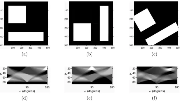
Subfigure (a), (b) and (c) show the input images, where (a) is the original, (b) (c) are rotated by 90 degrees and 30 degrees counter- clockwise, respectively. Subfigures (d), (e) and (f) are the visualized results of the transformation of (a), (b) and (c). . . 28

(16)

2.17 Visualized steps of the parallel method for multi-directional projections with fixed vector length. . . 33 2.18 Comparison of runtimes for different image sizes [K4]. The horizontal

axis displays the width of the squared images in pixels. The vertical axis shows the runtimes in milliseconds. The CPU and GPU imple- mentations of the presented method were compared with the runtime of MATLAB’s GPU-accelerated Radon transform [K4]. . . 36 2.19 The calculated horizontal, vertical, diagonal and antidiagonal projec-

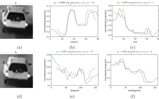
tions for different observations of the same vehicle. In subfigure (a) and (d) are imagesI₁ andI₂, in subfigures (b) and (c) the normalized vertical and horizontal projections, and in subfigures (e) and (f) the diagonal and antidiagonal projections are shown. Note the difference caused by the blink on the left side of the vehicle on I₂. [K5]. . . 38 2.20 The calculated horizontal, vertical, diagonal and antidiagonal projec-

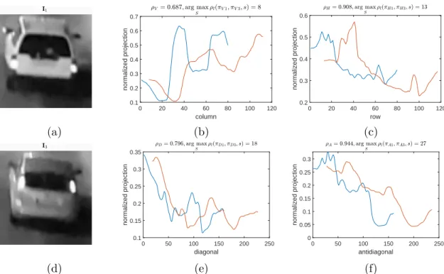
tions for observations of two different vehicles. In subfigure (a) and (d) are images I₁ and I₃ of the vehicles; in subfigures (b), (c), (e) and (f) the normalized vertical, horizontal, diagonal and antidiagonal projections are shown. Note the high correlation coefficients for the clearly different functions [K5]. . . 39 2.21 The measured correlation coefficients and calculated similarity scores

in the case of true pairs using the 4D signatures. The scatter plot in subfigure (a) shows the values of ρ_H and ρ_V. In subfigure (b), the diagonal ρ_D and antidiagonal ρ_A correlations are visualized. The µ similarity is presented in subfigure (c) [K5]. . . 40 2.22 The measured correlation coefficients in the case of false pairs using

the 4D signatures. Subfigure (a) shows a scatter diagram of measured ρ_H horizontal andρ_V vertical correlations. In subfigure (b) is a similar diagram with the diagonal (ρ_D) and antidiagonal (ρ_A) coefficients.

Note the large spread and high amount of very strong similarities.

Also, it is notable that the negative correlations are removed and corresponding values are set to zero [K5]. . . 41 2.23 A histogram of the distribution of the similarities calculated for the

same (red) and different (blue) objects [K5]. . . 41 2.24 Distributions of similarity scores generated by using alternatives to

the Euclidean norm (Figure 2.23). In the subfigure (a) the average, in (b) the maximum and in (c) the minimum values were used from the four calculated coefficients. . . 42 2.25 Histogram of the similarities measured using the multi-directional

projection method, with a fixed bin number of 25, andStepSizeset to five degrees. Red columns show the percentage for the comparison of the same and blue columns present the calculated values for different objects [K5]. . . 44 2.26 The rate of false positives if the threshold is adjusted to a limit where

50% (F50) or 80% (F80) of true matches should pass, for different number of projection bins [K5]. . . 45 2.27 A comparison of memory cost for the 2D and 4D signatures and the

multi-directional method with fixed bin numbers for different image sizes. . . 45

(17)

2.28 A selection of various false positive and false negative pairs [K5]. . . . 46 2.29 (a) Distribution of calculated similarity scores when using the Radon

transform to produce multi-directional projections. The step size used for rotation was five degrees. The scores are similar to the previously introduced 4D signature-based method, visualized in Figure 2.23. Di- agram (b) shows the differences between the two histograms. . . 48 3.1 The basic structure of the "two-headed" Siamese Neural Network.

The fully-convolutional (FCN) layers are followed by fully-connected (FC) layers. These heads share the same weights, and their outputs are multi-dimensional vectors. The distance of the output vectors gives the similarity of the inputs [K6]. . . 53 3.2 The sequence diagram of the interactions between the Master and

the Worker instances. After the Master starts, the Workers take new tasks from the waiting queue, process them, and send the results back. After there is no job left, the Worker gets notified by a so-called poison pill, and then terminates [K9]. . . 69 3.3 The estimated complexity values and the processing times for each

model, ordered by the estimated value based on (3.10). The thick red line represents the complexity value, while the thin columns show the processing times for each model. Although there are some visible diversions between the two, the calculated correlation is strong, 0.749 [K9]. . . 72 3.4 Correlation heatmap generated using the input parameters of model

training and the measured processing times from the total of 4000 trainings. pred represents the predicted complexity based on (3.10). . 73 3.5 A sample frame from the Vehicle ReIdentification dataset provided for

the International Workshop on Automatic Traffic Surveillance, on the 29th IEEE Conference on Computer Vision and Pattern Recognition (CVPR 2016) [112]. . . 74 3.6 Sample images from the dataset, from left to right: the original image,

the result of the Radon transform, the MDIPFL transform and the Trace transform, respectively. . . 76 3.7 One-shot classification accuracy for classes N = 1. . .10, grouped by

different numbers of hidden convolutional-pooling layer pairs, from 1 to 5, left to right, respectively. . . 79 3.8 Average processing times of models grouped by input types and the

number of hidden layers. Each bar represents the average processing time of the training 50 models twice. Error bars illustrate the standard deviation. . . 80 3.9 The results visualized by the number of parameters for the model

and the validation error rate. Each model was tested with 10,000 validation examples. The Pareto optimal results – values that are not dominated by any other result – are visualized in the bottom left corners as the Pareto frontier [K6]. . . 82

(18)

List of Tables

2.1 Processing of the projection calculation methods on different image sizes [K4]. . . 35 2.2 Runtime of the proposed method compared to the Radon transform

function in MATLAB [K4]. . . 36 2.3 Performance of the 2D and 4D projection signatures for object match-

ing. Note that the calculated similarity score is very high for the false pairs as well [K5]. . . 40 2.4 Performance of the multi-directional projections, with bin number set

as N, 2N-1, 25, 50, 100 and 300. As visible, constant bin numbers perform better [K5]. . . 43 3.1 The distributed processing of the models was done in two separate

runs. While there is a minimal difference between the results, the speedup and the efficiency in both cases are very high. It is also important to point out that the load balance of this scheduling is very good, the granularity of the last tasks is fine, causing a low idle time for the Worker which terminates first. Time values in this table are represented in a HH:MM:SS format [K9]. . . 71 3.2 The results of 1000 simulations of random scheduling. The generated

runtimes are ordered increasingly, and the minimum, maximum and median values are described in three columns of this table. Time values in this table are represented in a HH:MM:SS format [K9]. . . . 71 3.3 The different input types, by matrix sizes. As MDIPFL works with

a fixed bin size, multiple outputs were generated and tested. . . 75 3.4 The measured prediction accuracy for each transformation for 2,4,6,8

and 10-way classification. The models were tested with 10,000 tests and the best performances were selected for this table. . . 78 A.1 Top measured one-shot classification accuracy for different inputs dur-

ing N-way classification for one hidden convolutional-pooling layer pair.101 A.2 Top measured one-shot classification accuracy for different inputs dur-

ing N-way classification for 2 hidden convolutional-pooling layer pairs. 101 A.3 Top measured one-shot classification accuracy for different inputs dur-

ing N-way classification for 5 hidden convolutional-pooling layer pairs. 102

(19)

List of Algorithms

1 Method to calculate Multi-Directional Fixed Length Projections of an Image. . . 23 2 Kernel procedure to calculate the image projection for multiple direc-

tions. . . 31 3 Function to calculate the output size for a given input image with

the size given asI_W andI_H. L_num is the total number of convolutional-pooling layer pairs. C_W,C_H,P_W andP_H gives the maximum sizes of the convolutional kernels and pooling windows. . . 57 4 Method to calculate the maximum window sizes for a given input

image: L_num is the total number of convolutional-pooling layer pairs.

I_W and I_H denotes the input size and r_CP gives the minimum ra- tio between convolutional and pooling window sizes. The GetSize function is defined in Algorithm 3. . . 58 5 Searching for available solutions using a recursive backtracking search

with multiple results. . . 59 6 The estimation of the ideal batch size for training. The minimum

number of training batches is defined as 10; however, this could de- pend on the number of training samples in a single epoch. Function RoughEstimation results in the number of bytes defined in (3.7). . 61 7 The algorithm of the Master. For representation purposes, the inner

loop is an infinite loop, which accepts incoming TCP connections on the defined IP and port; however, in an actual software cancellation can be implemented as well for to shutdown of the listener. . . 66 8 Processing of the client requests is based on the first message of the

client: if the client states it is "ready," then a new task is sent to it.

In other cases, the worker is trying to send the results of a process. . 67 9 The pseudo language representation of the Worker process. The work-

ers repeatedly ask for the next neural architecture, and after training and evaluation, the results are sent back to the Master. Worker ter- mination is implemented with the "poison pill" approach. . . 68

(20)

Chapter 1 Introduction

Equations are just the boring part of mathematics.

I attempt to see things in terms of geometry.

— Stephen Hawking

Closed-circuit television cameras – also known as surveillance cameras – are often applied to monitor traffic. Based on the use cases, several applications of these traffic cameras are known: congestion-detection and accident-detection systems are popular, speed cameras, safety and various enforcement solutions as well [1]. Most of these solutions require the device to be able to identify or track the vehicle, which could be challenging depending on the brightness and weather conditions. Advanced devices have high-resolution cameras with infrared LEDs for night vision [2], also PTZ¹ cameras can be used to track object movement.

On distant locations like public roads, highways, bridges and tunnels simple static cameras are placed with non-overlapping fields of view. These camera-networks are mostly used to measure traffic after crossroads and calculate the average speed of vehicles based on the distance between the cameras and the time of observations [3].

Recognizing a vehicle by using the plate number is not always feasible [4]. In tunnels, where natural light is rare and colors are hard to detect, the usage of such high-level devices is not cost-efficient, giving similar low-quality images as other, less expensive cameras. The changes in lighting and vehicle movement can cause difficulties when matching the image representations, as well as different camera settings could reflect in errors.

1pan-tilt-zoom

(21)

In computer vision, there are simple methods to find objects with specific colors or shapes [5]. Most methods are based on lines or corners, or other keypoint-based descriptors extracted from template images. In the case of noisy and low-quality pictures, low-level techniques can be applied, for example, template matching [K1]

and histogram- or image projection-based comparison [6].

The improvement of the projection-based method can be done by increasing the number of projection angles. There are some well-known methods that provide a mapping from two-dimensional data to one-dimensional projections, like the Radon transform [7] [8]. This, however, in the case of a rectangular structure, gives different projection lengths for different angles [K2], affecting in the result matrix of the Radon transform (the sinogram) as blank areas.

In Chapter 2, a method that generates the multi-directional projections of a squared input is introduced. This transform has a similar result as the application of the Radon transform; however, the negative effects are removed with a fixed vector length. To demonstrate the robustness of this algorithm, a data-parallel implementation is also described and evaluated in Chapter 2, Section 2.2.

In the following section (Section 2.3), this method is used as an input for object matching in the case of vehicle images. The precision rate, memory efficiency and computation cost of the method is compared with the rates given by previously studied techniques.

As a second thesis group, in Chapter 3, a machine learning-based solution is designed and developed for the same problem, based on Siamese-architectured convolutional neural networks. To analyze the applicability of the projection-based neural comparison, a novel method to generate convolutional neural network (CNN) architectures is proposed (Section 3.2). A distributed environment with high parallel efficiency is designed and implemented (Section 3.3), where the networks with the generated architectures are trained and evaluated (Section 3.4).

1.1 Object matching

Richard Szeliski [9] declares object recognition as one of the most challenging tasks of computer vision. By defining the actual task, the problem can be object detection, instance or category recognition. If the size and visual representation of the sought object or objects are known, and the task is to locate these on the input image, the task is object detection. The most popular applications for object detection can be observed in digital cameras, smartphones or even on social network sites for face detection on images.

In the case of re-recognizing a previously examined object, the task is referred to as instance recognition. The process of determining that two visual objects represent the same entity is object matching [9].

To match object representations, a number of methods were introduced during the history of computer vision. The early approaches are summarized in the paper of Joseph L. Mundy [10], concluding that the basic detection methods, such as template matching and basic signal processing, were used to detect and match objects. Mundy also states that some of the early ideas were revisited later in the 1990s.

Modern approaches for object matching were done using geometric object descriptors, lines, edges, corners and other interesting keypoints.

In the following sections some of these methods are presented.

(22)

1.1.1 Color-based segmentation and matching

A simple solution for object segmentation is based on colors. If the foreground color of the object is different from the colors of the environment and the background, object boundaries can be easily marked.

These color-based segmentation methods [5] can be implemented based on the RGB² representation of colors; however, the HSI³ intensity-based model is a proper choice for these tasks.

After the object is separated, multiple procedures can follow to match the object of interest with a reference. Based on the color information, the color histograms of the two can be compared [11]. It is worth mentioning, that although the results for true pairs from the same collection of images are satisfactory, changes in lightning or small color changes can significantly change the measured distance between the two histograms. Another disadvantage of this matching method is that the shape and texture of the object is ignored [12], and as different images can have very similar color histograms, in these cases the defined similarity would result in a false positive match.

It is notable, that segmentation could also be done based on intensity, texture [13] or edges [14]. Modern approaches are based on trainable convolutional neural networks. Examples for semantic segmentation are fully-convolutional networks [15]

or to handle the computational expenses the U-Net structure [16] is often used.

If segmentation is done as a preprocessing step, beyond color data, distance functions based on the shape of the segmented object can be applied to match the representation with others. Such a method is given as the Edge Histogram Descriptor [17] where the relative distribution of different edge-types was used as a signature of the object.

1.1.2 Keypoints and feature descriptors

While color information is important, the human eye uses more information to rec- ognize objects [18]. Segmentation, categorization and instance detection is based on spatial information, as well as relationships with adjacent objects and the surrounding environment.

In computer vision algorithms the problem space is narrowed down, reducing the visual representation as possible. According to a survey by Mundy [10], the paradigm of detection switched from basic geometric descriptions to appearance features.

Image features are based on keypoints and descriptors. A keypoint is a point of interest that is invariant to rotation, translation, scale and intensity transformations.

The descriptor gives information about the region around this point.

Points of interest could be corners, line endings, or points on a curve where the curvature is locally maximal. Historically, the first corner detection method was presented by Hans P. Moravec [19] in 1977. The idea was that corners (and edges) could be detected locally using a small window: if the shifting of the window to any direction results in a large change in the intensity sum, a corner is detected. As only a 45-degree shift is considered, any edges not horizontal, vertical or diagonal

2Red-Green-Blue

3Hue-Saturation-Intensity

(23)

are incorrectly marked as corner points.

The Moravec detector is not isotropic, the response is not invariant to rotation.

An improved solution was presented by Christopher G. Harris and Mike Stephens [20] in 1988. To deal with the noise and possible rotations, a Gaussian window function was introduced. Using this window, all possible shifts should be examined; however, this step would have been computationally intense. So, instead, the first-order Taylor series expansion was used to approximate the value.

In 1994, Jianbo Shi and Carlo Tomasi [21] proposed a method based on the Harris detector, with a small and effective change on the scoring formula.

It is important to point out that both the Harris corner detector and the Shi- Tomasi detector are invariant to rotation; however, both are affected by input scaling. The scaling issue could be handled by storing external information about the region around the point of interest, for example, the patch size [22]. Other descriptors based on derivatives are often used as descriptors, like the Laplacian of Gaussians (LoG) or Difference of Gaussians (DoG) [23].

Scale-invariant feature transform (SIFT) was published by David G. Lowe in 1999 [24]. Inspired by the Harris detection, the procedure of feature extraction was based on the application of Gaussian kernels to obtain multiple scale representations of the same image, which was used to discard points of interest with low contrast.

The SIFT method is sensitive to lightning changes and blur, but the most important drawback of the application is that it is computationally heavy and real-time applications are not feasible.

The Speeded up robust features (SURF) [25] technique is using integral images resulting in a faster detection with similar precision [26]. It is worth mentioning, that the SURF method itself is not real-time; however, parallelization is possible.

If the task is matching instances of similar objects of the same category with similar appearance on low-quality images, the application of feature-based descriptors could result in low performance. While scale-invariant feature detection is a computationally intense process, noise of low contrast, blur and lightning changes affect the features, and therefore the result of matching as well.

For the vehicle-matching problem several solutions were introduced. For aerial object tracking, [27] introduced an extended line segment-based approach to detect and warp observations for matching. The authors proposed another approach in the following year based on 3D model approximation [28]. A similar method for vehicle matching of observations in different poses was introduced in [29], where the estimation is supported by the reflected light. In [30], it was pointed out that temporal information could also be used for tracking in a multi-camera network.

1.1.3 Template matching

To deal with the matching of low-quality images, classic template matching [31]

can be used. Finding the visual representation of an object on a reference image is based on a basic, pixel-level comparison of the reference pixels and the template.

The matching process is comparing the pixels of the template image with the reference image, using a sliding window, and selecting the best fit. The window is a template-sized patch, which is moved over the reference image.

While moving the window over the reference image, the fitting of the corresponding pixels is measured. There are several methods to evaluate: the simple ways are

(24)

to calculate the sum of squared differences or the cross-correlation. However, the normalized versions of these methods usually provide better results.

Depending on the chosen method, the minimum or maximum value represents the best match on the image. Multiple matches can be handled as well, if a threshold is applied instead of the minimum-maximum selection.

Template matching is sensitive to rotational or scalable changes on the reference image. A possible solution to solve the problems raised by different sizes is to create multiple images resizing the original template, match each of them on the reference, and, finally, select the best match of the results. These multi-scale template-matching methods are highly parallelizable [K3]. It is notable that this method could still fail detecting rotated or tilted objects.

1.1.4 Haar-like features

The processing of intensity values on an image patch is computationally expensive, and although parallelizational methods exist, the effectiveness is questionable. An alternative to working with intensities is based on integral images.

In 1997, Constantine P. Papageorgiou et al. presented a method [32, 33] which was based on the idea of Haar wavelets. After a statistical analysis of multiple objects from the same class, the trainable method was able to detect objects, for example, pedestrians or faces.

In 2001, Paul Viola and Michael Jones [34] published a machine learning approach to detect visual representations rapidly. Motivated by Papageorgiou et al. the system was not working directly with intensities, initially an integral image representation was computed from the source, storing the sum of pixel intensities for every point on the image.

The authors also defined Haar-like features [35] as differences in the sum of intensities in rectangular regions in an image. Using the integral image, the intensity sum of a rectangular region can be calculated in constant time, producing a fixed step number for Haar-like feature computation.

The Viola-Jones detector is trainable and uses an AdaBoost-based technique to select the important features and to order them in a cascade structure to increase the speed of the detection. The method was very popular and widely used from face detection to vehicle detection.

After the detection, the matching could be done based on the same features used for detection [36], without the need of unnecessary computation. Reyes Rios- Cabrera et al. [4] presented a complex system for vehicle detection, tracking and identification. In the identification method, a so-called vehicle fingerprint was used, which is based on the Haar-features used for detecting the vehicles.

The speed and accuracy of a system based on reusing Haar-like features are satisfactory; however, the condition of necessary pre-training is difficult to meet in real-life applications. The training set of images and the test set should be acquired on the same environmental conditions. Also, the set needs to be large enough to include multiple environments, conditions (lightning, weather, etc.).

(25)

1.2 Projection features

Similar low-level features could be constructed based on the sum of intensities for every column and row of the patch. These sums, the horizontal and vertical projections, are one-dimensional vectors mapped from the 2D image.

Applications of row and column sum vectors are first described by Herbert J. Ryser in 1957 [37], which is referred as one of the first discrete tomography [38, 39] methods: based on the two orthogonal projections, the original binary matrix is reconstructable. Reconstruction from a small number of projections can yield multiple valid results. It is notable that, in the case of a non-binary domain of values, the number of possible solutions of the reconstruction method can be lowered by more projections.

While reconstruction is important in medical applications [40], for object image matching the projection functions themselves could be used. Margrit Betke et al. presented a method for vehicle detection and tracking [41], where projection vectors are calculated of an edge map and are used to adjust the position during tracking.

In other applications, projections can be used for gait analysis for walking people [42], where the video sequence is transformed into a spatio-temporal 2D representation. Patterns in this so-called Frieze-group [43] representation can be analyzed using horizontal and vertical projections. As an extension, a variation of this method could be developed based only on the shape information [44], resulting in a method that was not affected by body appearance.

The idea of using a mapping of the vehicle observation for further processing also appeared in [45], where the distance calculation between observations were based on edge maps.

1.2.1 4D signature calculation

Vedran Jelača et al. [46] presented a solution based on projections for vehicle matching in tunnels, where object signatures are calculated from projection profiles. A possible interpretation of this method is presented here in detail.

After the region of interest is selected, the area is completed to a square and cropped. As color data are irrelevant in dark, artificially lighted areas such as tunnels, the images are grayscaled, meaning that the information is simplified from a RGB structure to a single intensity value. In the case of 8-bit grayscale images, the intensity information of one pixel is stored in one single byte.

Each image can be handled as matrixI∈N^N×N whereI_i,j = [0,1, . . .255] denotes the element of the matrix at (i;j). The horizontal (π_H) and vertical projections (π_V) for a squaredN ×N matrix result in vectors with the same length:

dimπ_H = dimπ_V =N. (1.1)

These projections are the averaged sums of the rows and columns of the matrix, normalized to [0,1] by the value of maximal possible intensity:

π_H(i) = 1 255N

N

X

j=1

I_i,j,

π_V(j) = 1 255N

N

X

i=1

I_i,j,

(1.2)

(26)

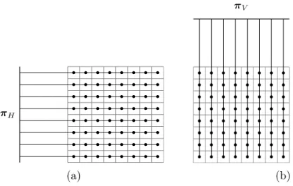
πH

(a)

πV

(b)

Figure 1.1. Horizontal (a) and vertical (b) image projections are calculated by summarizing the row and column values in the matrix.

πD

(a)

πA

(b)

Figure 1.2. Diagonal (a) and antidiagonal (b) image projections of a squared image matrix.

visualized in Figure 1.1.

π_H,π_V, therefore, defines the two-dimensional projection signature of the object:

S₂ = (π_H,π_V). (1.3)

The diagonal and antidiagonal projections can be calculated likewise, but it is important to point out that the number of elements for each projected value differs (Figure 1.2).

The length of the diagonal projection vectors are:

dimπ_D = dimπ_A= 2N −1, (1.4)

the number of elements in each summarization is based on the distance from the main diagonal:

ElemNum(i) =







i if i≤N

2N −i otherwise (1.5)

wherei is the index of an element in a diagonal projection, having i≤2N −1.

(27)

The calculation of the diagonal projections π_D,π_A is formalized as:

π_D(i) =











1 255·ElemNum(i)

Pi

j=1I_j,N_−(i₋_j) if i≤N

i−N

P

j=1I_j+(i₋_N),j otherwise

π_A(i) =











Pi

j=1I_j,(i₋_j)+1 if i≤N

i−N

P

j=1I_j+(i₋_N),N_−(j₋₁₎ otherwise

(1.6)

These projection vectors together provide the 4D projection signature of the object:

S₄ = (π_H,π_V,π_D,π_A). (1.7) After normalizing the values using the number of elements that make up the sum, multiplied with the maximum intensity value 255, the domain of the projection function is [0; 1]. The 4D signature of a vehicle observation is visualized in Fig. 1.3.

1.2.2 Projection-based object matching

As the size of the input images could be different, the length of projection functions is different as well. To be able to match these functions properly a similarity measurement method must be defined.

Cropped image

(a)

0 20 40 60 80

column 0.1

0.2 0.3 0.4 0.5 0.6 0.7

normalized projection

Vertical projection

(b)

0 20 40 60 80

row 0.25

0.3 0.35 0.4 0.45 0.5 0.55

Horizontal projection

(c)

0 50 100 150

diagonal 0.1

0.15 0.2 0.25 0.3 0.35

Diagonal projection

(d)

0 50 100 150

antidiagonal 0

0.05 0.1 0.15 0.2 0.25 0.3

Antidiagonal projection

(e)

Figure 1.3. The visualized projection signature of a vehicle observation. Subfigure (a) shows the squared image of a rear-viewed vehicle. In diagrams (b), (c), (d) and (e), the horizontal, vertical, diagonal and antidiagonal projections are visualized (π_H, π_V, π_D and π_A, respectively).

(28)

To calculate the alignment of the functions, the method suggested in [46] is to align the projection functions globally, and then fine-tune with a "local alignment"

using a method similar to the Iterative Closest Point [47, 48].

First, the signature vectors are rescaled based on the camera settings and the position of the object in the image, so the effects of zoom and camera settings are corrected. After the signatures are resized, it is still necessary to align the signatures because of shifting and length differences.

The functions are compared based on the sliding window technique: the shorter function is moved over the longer function, and each correlation coefficient is calculated using the Pearson correlation coefficient (PCC) formula:

ρ_l(x,y, s) = cov(x,y_s)

σ(x)σ(y_s), (1.8)

where x,y are projection vectors, where dimx ≤ dimy. y_s represents the part of vectory, which is shifted by s and overlaps x.

Basically, the ρ_l(x,y, s) correlation coefficients are calculated for each step s, where the number of steps is dimy−dimx. cov(x,y_s) means the covariance between the two vectors and σ indicates the standard deviation.

The highest value max_sρ_l(x,y, s) is selected asρ, defining the similarity ofxand y. For horizontal, vertical, diagonal and antidiagonal projection functions, notations ρ_H,ρ_V, ρ_D and ρ_A are used, respectively.

The local alignment suggested in [46] was based on signature smoothing followed by curve alignment: step-by-step iteratively removing the extremas caused by noise and finding the best fit for two functions.

The range of the values are mapped to [−1; 1], which could be easily handled: the higher the coefficient, the better the match. After all similarity values are calculated for the projections, the result values are filtered with a rectifier, setting all negative values to zero:

r(v) =







v if v >0

0 otherwise = max(0, v) (1.9)

Negative correlation values mean that the changes of one function affect an opposite change on the other function, meaning that the relationship between the two is inverse. So, in this case, the penalization of the negative correlation is necessary, because projection inverses should not be relevant at all.

The suggestion in [46] is to equally handle each dimension of the data, by using the Euclidean norm (L2 norm). A single similarity value µ is calculated from the 4D signature as

µ=

qr(ρ_H)²+r(ρ_V)²+r(ρ_D)²+r(ρ_A)²

2 (1.10)

where 2 is the square root of the dimension number, therefore, normalizing the norm.

1.3 Goal of the research

The research described in the following chapters was inspired by this four-dimensional projection signature technique. The motivation for further research was based on the study of multiple projection directions for object descriptors.

(29)

The main goal is to analyze the effectiveness of multi-directional projection signatures for object matching. As the four-dimensional projection signatures are applicable for instance recognition, it is presumed that multiple directions would increase the accuracy of the method.

The length of a projection vector depends on the size of the image and on the projection angle. If the calculated similarity of different length functions is based on the best fitting, the resulting values result in high scores even in the case of false pairs.

My goal is to develop a multi-directional projection mapping method, where the number of bins is independent from the rotational angle or the image size.

The properties of the designed transformation should be analyzed and the performance of object matching should be compared to other similar techniques.

The possibilities of parallel implementation should also be examined, as modern computer architectures provide great support for data-parallel execution.

For different object types, projections could have different significance in terms of object matching. To analyze the weight of each angle, statistical or machine learning approaches could be done.

The secondary goal of this dissertation is to study the modern machine learning approaches of object matching and to analyze the applicability of multi-directional projections for object descriptors for the same task.

A comprehensive experiment is necessary to determine the performance of such methods. In large experiments, the selective environment and the broad input data are key factors. In this dissertation, a complex experiment is designed and implemented for object image matching using neural networks.

As a part of this task, a neural network architecture generation method is developed and a distributed approach for processing the models is designed.

(30)

Chapter 2 Multi-directional image projections

Good approximations often lead to better ones.

— George Pólya, Mathematical Methods in Science

While projection-based matching methods can be simply described and implemented, the noise of surrounding objects and lighting changes result in noise, which affects the precision of the solution. In works presented earlier [4, 45, 46], these draw- backs are handled by complex appearance modeling and multiple levels of alignment during the process.

It is clear that the computational cost of the projection transformation is low and data-parallel solutions could be given to further reduce the runtime. However, the complexity of the matching algorithm alongside the rescaling, noise removal and alignment steps significantly affect the overall performance.

The idea of increasing the number of projections was motivated by the mechanism of computer-assisted tomography machines: the more input data is given, the more precise the reconstructed 3D image is going to be. More accurately, there is a tradeoff between accuracy and computational cost, and the latter is directly affected by the number of projection angles.

In the following sections, the well-known Radon transform is introduced and analyzed, followed by the definition of a novel method for multi-directional image projection calculation in Section 2.2. To demonstrate the real-time capabilities of the method, a data-parallel solution is given in Section 2.3. The method is implemented and results for object matching are evaluated in Section 2.4.

(31)

2.1 Introduction

For horizontal and vertical projections on rectangular patches, the summarization of rows and columns is a correct approach. In case the diagonal and antidiagonal projections are also required in a squared matrix, the method of summarizing elements by traversing through the matrix as given in Section 1.2 is similarly simple.

For other angles (i.e. other than 0, 45, 90, 135 degrees), this discrete, element- based method is not applicable without direct loss of information or ambiguity.

The solution for this problem can be based on the work of mathematician Johann Radon, who defined a mathematical framework to create a transformation between an object and its projections [40].

2.1.1 The Radon-transform

The original mapping of 2D objects to 1D projection profiles was first studied by Johann Radon [7] in 1917; a translation of his paper was published in 1986 [8]. The formula and the inversion formula became popular [40] as they were used with CT¹, PET², MRI³ and SPECT⁴ scanners to reconstruct images from the obtained data.

Current reconstruction algorithms are based or inspired by the inverse Radon-transformation [40]. Other application fields include electron microscopy [49], astronomy [50], and geophysics [51].

To formally define the method, define f as a function on the two-dimensional Euclidean space R². Let (x, y) designate coordinates of points of the plane. The Radon transform off results in ˇf by integrating f over all L lines in the plane.

So the Radon transform is usually defined as fˇ=Rf =

Z

L

f(x, y)ds, (2.1)

The projection or line integral is based on line L ∈ R², and ds is an increment alongL[40]. It is notable, that there are multiple generalized forms of the transform, where the domain is extended to higher dimensions (such asR² or Rⁿ) [52, 53].

A line could be given in normal form as

p=xcos(φ) +ysin(φ), (2.2)

whereφ is the angle of rotation. From pand φ, the Radon transform off(x, y) can be given as

f(p, φ) =ˇ Rf =

Z

L

f(x, y)ds. (2.3)

A rotated coordinate system with axes p and s could be presented by applying the rotation matrixRot(φ) as

1Computerized Tomography

2Positron Emission Tomography

3Magnetic Resonance Imaging

4Single-Photon Emission Computed Tomography

Óbuda University