1.Introduction M.V.Barbarossa, M.Polner, andG.Röst TemporalEvolutionofImmunityDistributionsinaPopulationwithWaningandBoosting ResearchArticle

(1)

Research Article

Temporal Evolution of Immunity Distributions in a Population with Waning and Boosting

M. V. Barbarossa,¹M. Polner ,²and G. Röst^2,3

1Institute for Applied Mathematics, Heidelberg University, Im Neuenheimer Feld 205, 69120 Heidelberg, Germany

2Bolyai Institute, University of Szeged, Aradi vértanúk tere 1, Szeged 6720, Hungary

3Mathematical Institute, University of Oxford, Woodstock Road, Oxford OX2 6GG, UK

Correspondence should be addressed to M. Polner; polner@math.u-szeged.hu Received 24 January 2018; Accepted 2 July 2018; Published 30 August 2018

Academic Editor: Philippe Bogaerts

Copyright © 2018 M. V. Barbarossa et al. This is an open access article distributed under the Creative Commons Attribution License, which permits unrestricted use, distribution, and reproduction in any medium, provided the original work is properly cited.

We investigate the temporal evolution of the distribution of immunities in a population, which is determined by various epidemiological, immunological, and demographical phenomena: after a disease outbreak, recovered individuals constitute a large immune population; however, their immunity is waning in the long term and they may become susceptible again.

Meanwhile, their immunity can be boosted by repeated exposure to the pathogen, which is linked to the density of infected individuals present in the population. This prolongs the length of their immunity. We consider a mathematical model formulated as a coupled system of ordinary and partial differential equations that connects all these processes and systematically compare a number of boosting assumptions proposed in the literature, showing that different boosting mechanisms lead to very different stationary distributions of the immunity at the endemic steady state. In the situation of periodic disease outbreaks, the waveforms of immunity distributions are studied and visualized. Our results show that there is a possibility to infer the boosting mechanism from the population level immune dynamics.

1. Introduction

The outcome of an infection within an individual host depends on the speciﬁc pathogen and the status of the immune system of the host. At a larger scale, the outcome of an epidemic in a population is inﬂuenced by the ensemble of individual immunities. There are a number of processes in play that determine how these immunities change in time.

Upon recovery from infection, some immune memory remains, which may persist for long time after pathogen clearance. Eventually, memory cells slowly decay, and in the long run, recovered hosts could lose pathogen-speciﬁc immunity [1]. Waning immunity is possibly one of the contributing factors which cause, in particular in highly developed regions, recurrent outbreaks of infectious diseases such as chickenpox and pertussis. Immune memory can be boosted due to repeated exposure to the pathogen thus prolonging the time during which immune hosts are protected. Our goal in this paper is to monitor the distributions of immune memories in a population and

track their temporal evolution, which provides very important insights about the interplay of individual and population level disease dynamics.

In the SIR framework, a population of hosts is divided into susceptibles (S), infectives (I), and recovered (R), and interactions among individuals from the diﬀerent compartments are considered. Susceptibles are those hosts who either have not contracted the disease in the past or have lost immunity against the disease-causing pathogen. When a susceptible host gets in contact with an infective, the pathogen can be transmitted and the susceptible host may become infective.

After the loss of immunity, an individual from compartment Rtransits back to the susceptible compartment; hence when waning of immunity is included, the model is calledSIRS.

To account for immune system boosting, we structure the immunes according to their level of immunity. The high complexity of the immune status of an individual is simpliﬁed into a single parameter that reﬂects the strength of immunity in the sense that it indirectly indicates the duration of immunity until waning. The challenge due to

Volume 2018, Article ID 9264743, 13 pages https://doi.org/10.1155/2018/9264743

(2)

secondary or multiple exposures to the pathogen initiates an immune response that results in a higher level of immunity.

The details are yet unclear how exactly the immune response and in particular a boost of the immune system work [1]; most likely, there is a range of mechanisms underlying these processes that are speciﬁc to each host and pathogen [2]. Laboratory analysis on vaccines tested on animals or humans suggests that the boosting eﬃcacy might depend on several factors, among which the current immune status of the recovered host and the amount of pathogen he receives [2, 3]. In previous mathematical models, it was assumed that a boost restores the maximal immune status, the same as after natural infection [4]. Few authors have assumed that at each new contact with a known pathogen, the immune system is boosted a little, with a small increase in memory cells [5]. Others have considered a combination of both possibilities [6].

To investigate the temporal evolution of how the distribution of these immunity levels changes in the population, we propose a mathematical modeling framework along the lines of our previous works [7, 8]. The core of the model is a hybrid system of equations of SIRS type, in which the immune population is structured by the level of immunity, whereas the susceptible and the infective populations are nonstructured. In [8], we investigated the well-posedness of the general model and its basic qualitative properties, whereas in [7], we considered a special case of the hybrid system in form of delay diﬀerential equations (DDEs) with constant and distributed delay. Here, we focus on the immune response identifying several possible scenarios for immune system boosts.

We systematically compare a number of assumptions on the boosting mechanism that have been used in the literature.

The goal is to observe the effects of different immune responses not only at an individual but also at population level, such as the stationary distribution of immunities in the case of an endemic disease and the periodic change of these distributions in case of repeated disease outbreaks. To the best of our knowledge, there are no further studies about the temporal evolution of the distribution of immune statuses in a population, and the only paper that has predicted a spe- cific immunity distribution from a mathematical model is [6].

In Section 2, we provide the details of the mathematical model and present the numerical methods that are used for its solution. Four scenarios for immune boosting mechanisms are described and compared in Section 3, together with the parametrizations that lead to an either stable endemic state or oscillatory disease outbreaks. A careful and system- atic numerical analysis is performed to understand the eﬀect of various boosting mechanisms, and the results are summa- rized and discussed in Section 4.

2. Materials and Methods

2.1. The Mathematical Model.LetS t and I t denote the total population of susceptibles and infectives, respectively, at time t. The total population shall be assumed to be in balance (hence normalized) N t ≡1, with birth rate equal

to the natural death rated≥0and no disease-induced death.

We assume that newborns are all susceptible.

Contact with infectives (at rateβI) induces susceptible hosts to become infective themselves. Infected hosts recover at rate γ> 0, that is, 1/γ is the average infection duration.

Once recovered from the infection, individuals become immune; however, there is no guarantee for life-long protection. Immune hosts who experience immunity loss become susceptible again.

Let r t,z denote the density of immune individuals at time t with immunity level z∈ z_min,z_max, 0≤z_min<

z_max<∞. The total population of immune hosts is given by

R t = ^z^max

z_min

r t,z dz 1

The parameterzdescribes the immune status and can be related to the number of speciﬁc immune cells of the host.

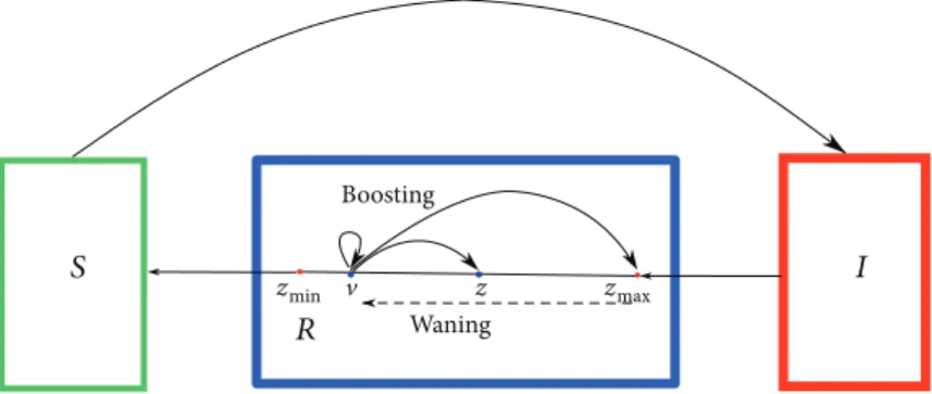
The value z_max corresponds to the maximal immunity, whereas z_min corresponds to the lowest level of immunity for hosts in theRcompartment. We assume that individuals who recover at timetenter the immune compartment with maximal level of immunityz_max. The level of immunity tends to decay in time and when it reaches the lower thresholdz_min, the host becomes susceptible again. However, contact with infectives, or equivalently, exposure to the pathogen, can boost the immune system fromz∈ z_min,z_max to any higher immune status (see Figure 1).

Given a host withinitialimmune statusv∈ z_min,z_max, let us denote byZ^v∈ z_min,z_max theupdatedimmune status, which is achieved after new contact with the pathogen. The updated immune statusZ^vis modeled as a random variable taking values in S_v≔ v,z_max ⊆ z_min,z_max ⊆ℝ with probability density function p ·,v . The value p z,v represents the relative likelihood that a boost from immune level vto level z occurs. Secondary exposures to the pathogen might have no eﬀects on the host’s immune system or might restore the immunity level induced by the disease (z_max). In order to capture these particular aspects, in Section 3.1, we shall also consider limit cases in which the probability density function is a Dirac measure centered either on the current immune status or on the maximal levelz_max.

The immunity level decays in time at rate g z, with g positive, smooth, and bounded, which is the same for all immune individuals with immunity level z. In the absence of immune system boosting, an infected host who recovered at timet₀becomes again susceptible at timet₀+τ, where

τ= ^z^max

z_min

1

g x dx 2

With the above assumptions, we obtain for t> 0 the following system of equations

S′ t =d 1−S t −βS t I t +g z_min r t,z_min ,

I′ t =βS t I t − γ+d I t , 3

(3)

with initial valuesS 0 =S⁰> 0,I 0 =I⁰≥0, coupled with a partial diﬀerential equation (PDE) for the immune population,

∂

∂tr t,z − ∂

∂z g z r t,z =−dr t,z +βI t

z z_min

p z,v r t,v dv−r t,z ,

4 forz∈ z_min,z_max, with boundary condition

g z_max r t,z_max =γI t , 5

and initial distribution r 0,z =ψz ,z∈ z_min,z_max. A sketch of the full model is given in Figure 1, whereas some possible boosting mechanisms are depicted in Figure 2, and they will be discussed later in detail. The formal derivation of a slightly more general version of models (3), (4), and (5) with variable total population size and disease-induced death is given in [8].

2.2.R₀.Before presenting further results, we introduce the basic reproduction numberR₀of models (3), (4), and (5),

R₀= β

γ+d, 6

which indicates the average number of secondary infections generated in a fully susceptible population by one infected host over the course of his infection. The basic reproduction number is a reference parameter in mathematical epidemiology used to understand if, and in which proportion, the disease will spread among the population.

2.3. Numerical Solution of the Hybrid System.In the following, we outline the numerical method used to solve the hybrid system (3), (4), and (5).

Consider (3), (4), and (5) as a one-dimensional, ﬁrst- order nonlinear PDE system. In this section, we refer to the

independent variables t,z as time and space, respectively.

AsSandIdo not depend onz, but only on time, the initial conditions are

S 0,z ≡S0 ≡S⁰> 0, I 0,z ≡I 0 ≡I⁰≥0,

r 0,z =ψz , z∈ z_min,z_max

7

Sinceg z > 0for allz∈ z_min,z_max,the boundary condition forris imposed in (5) at the inflow boundary, that is, at z=z_max. All together we have an initial-boundary value problem (IBVP). For the numerical integration of the IBVP, we employ the MATLAB code hpde[9], developed to solve IBVPs for first-order systems of hyperbolic PDEs in one space variable and time. The hpde routine implements Richtmyer’s two-step variant of the Lax-Wendroff method [10, 11], which is well established to solve hyperbolic PDEs.

This scheme is explicit and second-order accurate in both space and time. To compute the numerical solution of our IBVP, we have modified the codehpdeso that the integral term in (4) is efficiently implemented, preserving the second-order accuracy of the Lax-Wendroff scheme. In Section 3.3, we have verified the spatial order of accuracy for a number of computations.

In the computation of the numerical solutions of the IBVP, we used an equidistant mesh z_min=̂z₀<̂z₁<⋯<

̂

z_M=z_max,Δ̂z=̂z_i−̂z_i−1,i= 1,…,M The initial function on this mesh is given by S 0 ,I 0 ,r 0,̂z_i = S⁰,I⁰,ψ̂z_i

For an explicit scheme for a hyperbolic system, a necessary condition for stability is the Courant-Friedrichs- Lewy condition, which for our system means

Δt Δ̂z max

̂z∈ ̂z₀,…,̂zM

g ̂z < 1 8

We deﬁne the boosting matrix Π as the numerical discretization of the probability density function p on the

zmin v z zmax

Boosting

Waning

Figure1: Sketch of the mathematical models (3), (4), and (5). Susceptible hosts become infective after pathogen transmission.

Infected hosts who recover enter the immune compartment R which is structured by the level of immunity. Natural infection induces the maximal level of immunity z_max. Immunity decays in time and when the immune status reaches the minimal value z_min; the recovered host becomes susceptible again. Meanwhile, exposure to the pathogen can boost the immune system and prolong protection.

(4)

equidistant meshΔ̂z. Each entryπij=Πi,j of the boosting matrix represents the probability that ̂z_i is the updated immune level, given initial immune level ̂z_j, that is, πij= p ̂z_i,̂z_j . It follows that πij∈ 0, 1, with πij= 0 if j>i and

〠^M

i=1πij=〠^M

i=jπij= 1, for allj= 1,…,M 9

3. Results and Discussion

3.1. Scenarios for the Immune Response. Let us consider an immune host who has immune status vat the moment of reexposure to the pathogen. We shall investigate the following possible scenarios for immune response in case of secondary exposure to the pathogen.

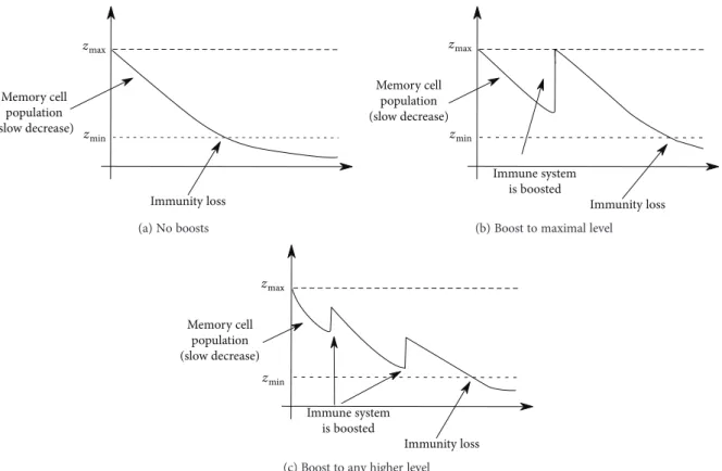
3.1.1. NOboost. Assume that the immune system does not respond to reinfection, that is, we observe only waning of immunity after recovery (Figure 2(a)). This corresponds to the limit case in which the boosting probability function is simply a Dirac measure with support on the initial immune level. It follows that (4) reduces to

∂

∂tr t,z − ∂

∂z g z r t,z =−dr t,z 10

Recall the deﬁnition of τ> 0 in (2). The transport equation (10) with boundary condition (5) is solved along characteristics and we obtain

g z_min r t,z_min =γI t−τ e^−dτ, 11

meaning that τtime after recovery immune hosts who did not die become susceptible again. In turn, we ﬁnd a delay term in the equation forSand have a classical SIRS model with constant delay (cf. [12])

S′ t =d−βS t I t −dS t +γI t−τ e^−dτ, I′ t =βS t I t − γ+d I t ,

R′ t =γI t −γI t−τ e^−dτ−dR t ,

12

whereR t is the total immune population at timetas in (1).

3.1.2. MAXboost.Assume that at any new encounter with the pathogen the immune system of a recovered host is boosted in such a way that the disease-induced (maximal) immunity is restored (Figure 2(b)). This corresponds to the limit case in which the boosting probability function is a Dirac measure with support on the maximal immune level (z_max). As

Immunity loss z_max

z_min Memory cell

population (slow decrease)

(a) No boosts

Immunity loss z_max

zmin

Memory cell population (slow decrease)

Immune system is boosted (b) Boost to maximal level

Immunity loss z_min

z_max

Memory cell population (slow decrease)

Immune system is boosted

(c) Boost to any higher level

Figure2: Exposure to the pathogen has a boosting eﬀect on the immune system, whereby several possible scenarios are possible: (a) No boosting events (NOboost): the host who recovered at timetbecomes susceptible at timet+τ, withτ> 0given in (2). (b) Boosts restore disease-induced immunity, that is, the immune system is always boosted to the maximal level of immunity (MAXboost). (c) Variable boost, to any higher immune level.

(5)

p(z,v)

z v

01

1 0.5

0.5 0.5

1

0 0 (a) ANYboost

Initial immune level (v)

0.40 0.1 0.2 0.3 0.4 0.5 0.6 0.7 0.8 0.9 1 0.5

0.6 0.7 0.8 0.9 1

Updated immune level (z)

(b) Nonmonotonic boosting functions

01

0.5 1

0.5

p(z,v)

0.5 0 0

1

z

v (c) ODboost

0 1

0.5 1

0.5 0.5

p(z,v)

0 0 1

z

v

(d) HKboost

Figure 3: Nonmonotonic immune response mechanisms. (a, c, d) Examples of diﬀerent boosting matrices Π for the numerical implementation ofp z,v, the probability that individuals with immune levelvat exposure are boosted to levelz≥vafter exposure. The immune status is represented in z_min,z_max = 0, 1 and discretized on an equidistant mesh with 30 points. (b) The dotted curve represents the boosting mechanism inspired by [6], the solid curve the one inspired by [14].

all boosted individuals are transferred to the boundary, and the integral term in (4) moves to the boundary condition, yielding

∂

∂tr t,z − ∂

∂z g z r t,z =−dr t,z −βI t r t,z , 13 g z_max r t,z_max =γI t +βI t R t 14 The BVP (13) and (14) can be solved along characteristics and one obtains fort≥0a system of delay equations with constant and distributed delay:

S′ t =d 1−S t −βI t S t

+I t−τ γ+βR t−τ e^−dτ−β ⁰^−τ^{I t+u du}, I′ t =βI t S t − γ+d I t ,

R′ t =−dR t +γI t

−I t−τ γ+βR t−τ e⁻^d^τ−β ⁰^−τ^{I t}⁺^{u du}, 15 withτ> 0as defined in (2) and with given initial functions ϕ^S t ≥0,ϕÎ t ≥0, andϕ^R t ≥0, such thatϕ^S t +ϕÎ t + ϕ^R t ≡1, for allt∈ −τ, 0. The formal derivation of system (15) is given in [7, 8].

3.1.3. ANYboost. We assume that the immune system is boosted to any better immunity level with uniform probability. That is, p z,v =p> 0 with p= 1/ z_max−v , for all z∈ v,z_max. The boosting matrix for the numerical implementation is shown in Figure 3(a).

3.1.4. HKboost and ODboost.Previous works have proposed nonmonotonic functions for modeling the immune response to secondary exposure. In [6, 13], a mathematical model for

(6)

in-host dynamics during measles infection was proposed.

The model explicitly considers the relation between the immune level at time of exposure and the level of memory cells after exposure. Heffernan and Keeling [6, 13] suggest that this relation is nonmonotonic. Indeed, although the level of immunity after exposure is always greater than the level at the time of exposure, the boosted level starts high, decreases, and then increases again. We shall denote by HKboost the boosting function from [6, 13]. For the numerical implementation of HKboost, wefirst extract values from Figure 2(d) in [6], which shows the relation between the initial and the updated immune status. Then, we normalize the immune status interval (z_min,z_max = 0, 1) and extend the boosting function to [0.75, 1], assuming that for high initial immune status, the immune system is always boosted to the maximal level (see Figure 3(b)). In terms of our model coefficients, for any initial immunityv, the atomic measure of the updated immunity is concentrated on f v , where f is the boosting function represented by the dotted curve in Figure 3(b).

The corresponding boosting matrix is shown in Figure 3(d).

Immune boosting in pertussis was considered in [14], where a nonmonotonic boosting function similar to the one in [6, 13] was proposed. The relation between the level of memory cells before (v) and after (z) reexposure is governed by the function

z=f v =v 1 + 1 5v

5, withv∈ 0, 5 16

De Graaf et al. [14] suggest that a small jump fromvtoz corresponds to a mild infection that causes no harm but only boosts the antibody level of the individual, whereas a large jump corresponds to a severe infection that may also cause disease. We shall use the boosting function in (16) for simulations, previous normalization to z_min,z_max = 0, 1 , and small modiﬁcations which allow to have boundedness.

In detail, we assume that for very low initial immunity (0≤v< 0 075) and for large initial immunity (0 8 <v≤1), the immune status is always boosted to the maximal level z=z_max= 1, whereas forv∈ 0 075, 0 8, the boosting probability is atomic along the graph of the boosting function f in (16), as above. The resulting boosting function is given by the solid curve in Figure 3(b), and the corresponding boosting matrix is shown in Figure 3(c).

The two mechanisms for immune response HKboost and ODboost are governed by rather similar boosting mechanisms, and we shall see that the solutions behave accordingly.

3.2. Parameter Values. For the numerical computations below, we set the birth rate, natural death rated= 0 02, and the initial conditionsψ₀ z = 0 05forz∈ z_min,z_max = 0, 1, I⁰= 0 01, and S⁰= 0 94. This means that we assume that 1% of the total population is infectious at the beginning of our observations, while 5% is immune to the pathogen and the level of immunity is equally distributed.

Concerning the disease dynamics, we set γ= 3 and g z = 0 5, for all z∈ z_min,z_max, corresponding to τ= 2 when the model can be reduced to DDE.

We allow the basic reproduction number R₀ as given in (6) to vary, in order to show both solutions that con- verge to an endemic equilibrium and solutions that produce periodic oscillations.

3.3. Stable Endemic Equilibrium.When the basic reproduction number is sufficiently small, the solution converges to an endemic equilibrium for all the boosting mechanisms presented in Section 3.1. We compare in Figure 4 the numerical solution corresponding to different boosting mechanisms. In Figure 4(a), we show the componentIof the solution, which indicates how the number of infective evolves in time and rapidly converges to an equilibrium. Changing the boosting mechanism has small effects on the infective population:

numerical solutions show the same qualitative behavior, with endemic equilibria deviating less than 1% from each other. In particular, we see that the nonmonotonic boosting mechanisms, ODboost, HKboost, and ANYboost, yield quantitatively equivalent solutions for the infective population. The latter solution curves are bounded from below by the solution of MAXboost and from above by the solution of the NOboost problem.

In Figure 4(b), for each boosting mechanism, we visualize the stationary distributionr z corresponding to the endemic equilibrium in Figure 4(a). This indicates how immunity is distributed among theR-population at the endemic equilibrium. It is visible that the choice of the boosting mechanism importantly aﬀects the stationary distribution. To understand why this happens, let us consider the case of a constant immune decay rate, g z =g, for all̂ z∈ z_min,z_max. For certain choices of the probability density function, p one can calculate the stationary distribution r z explicitly. For example, in the absence of immune boosts (NOboost), we have

r z = γI^∗

̂

g e⁻^d/̂^{g z}^max^−z, 17 where I^∗ is an endemic equilibrium of the systems (3) and (10), with boundary condition (5).

In case of boosts to maximal immune level (MAXboost), from (13) and (14), we have

r z =I^∗

̂

g γ+β 1− 1

R₀ −I^∗ e⁻^d+βI^∗^/̂^{g z}^max^−z , 18 with the basic reproduction number R₀=β/γ+d , as in (6). With the parameter values indicated in Section 3.2, and R₀= 1 5,the curves in (18) and (17) are almost straight lines, as it can be observed in Figure 4(b).

We use the analytic stationary solution (18) of systems (3), (4), (13), and (14) to verify the order of“spatial”accuracy (i.e., with respect to the variablez) of the numerical discretization. On different meshes, we compute numerically the stationary solution of the MAXboost systems (3), (4), (13), and (14). Although we know the explicit solution for the stationary distribution r, there is no explicit analytical for- mulation for the endemic equilibrium I^∗, which can only be determined numerically (see also [7]). We fixI^∗ to the value computed on thefinest mesh (M= 14000equidistant

(7)

mesh points), and we insert this value into the (18) of the stationary distribution. Then, we compute the maximum error between the analytical and the numerical solutions on different mesh refinements and observe that our method preserves the second-order accuracy of the Lax-Wendroff scheme (see Figure 5).

3.4. Sustained Oscillations, Repeated Outbreaks. When R₀= 5 and all other parameter values are as indicated in Section 3.2, the systems (3), (4), and (5) show periodic oscillatory behavior, independent on the boosting mechanism. In Figure 6, we compare theIcomponent of the solution of the systems (3), (4), and (5) forﬁve diﬀerent immune responses.

Further, for all kinds of immune response, we compare in Figure 7 the distribution of immune status among the

Mesh size (×10⁻⁴) Max error (×10−4)

1.5

0.6 0.8 1 1.2 1.4 1.6 1.8 2

1 2 2.5 3 3.5 4.545 5.5

Errors Least squares fit

2 1

Figure 5: Spatial accuracy of the numerical discretization, with error represented in a log-log plot. The method is second-order accurate.

0 5 10 15 20 25 30

Time (t) 0

0.1 0.2 0.3 0.4 0.5 0.6

I (t)

NOboost ANYboost MAXboost

ODboost HKboost

Figure 6: Infective population I t for diﬀerent boosting mechanisms. Also in case of periodic oscillations, it is evident that the solution of problems governed by the boosting mechanisms ODboost and HKboost are quantitatively equivalent.

Time (t) 0.01

0.02 0.03 0.04 0.05 0.06 0.07

I (t)

Infective population

ODboost HKboost

0 5 10 15 20 25 30 35 40 45 50

(a)

ODboost HKboost

0 0.1 0.2 0.3 0.4 0.5 0.6 0.7 0.8 0.9 1 z

0.22 0.24 0.26 0.28 0.3 0.32 0.34 0.36

r (z)

Stationary distribution

(b)

Figure4: Comparison of diﬀerent boosting mechanisms in case of a stable endemic equilibrium. (a) The infective population in case of NOboost (black curve), MAXboost (green), ANYboost (red dotted), ODboost (blue), and HKboost (magenta). (b) The stationary distribution in the immune populationr z corresponding to (a).

(8)

population for ﬁxed times (t= 1, 5, 10, 20 years) after the beginning of the observation. Results illustrated in Figures 6 and 7 and Table 1 indicate that also in the case of periodic oscillations, the solutions of problems governed by ODboost and HKboost are qualitatively and quantitatively equivalent (minor diﬀerences might be due to computational errors and we consider them negligible).

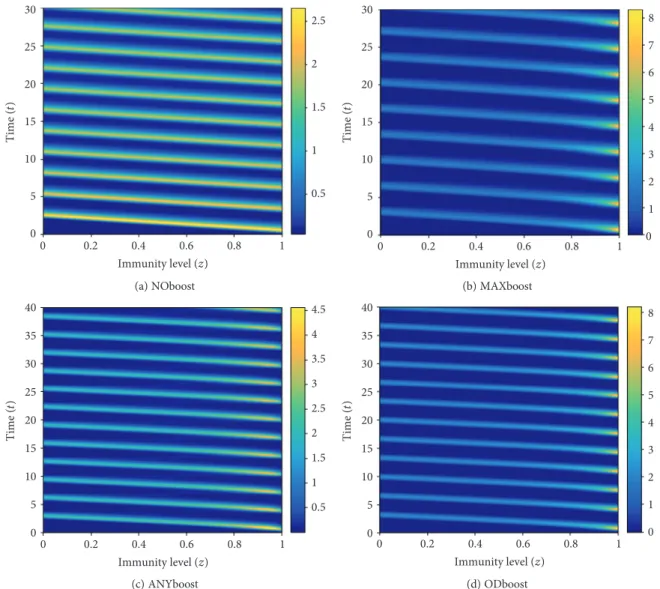
Therefore, in the following, we show only results related to NOboost, ANYboost, MAXboost, and ODboost, which characterize four diﬀerent immune responses with qualitatively diﬀerent results. Figure 8 shows the solution r t,z

z NOboost

ANYboost MAXboost

ODboost HKboost

0 0.2 0.4 0.6 0.8 1

0 1 2 3 4 5 6

r (t,z) at t = 1

(a)t= 1

ODboost HKboost z

0 0.2 0.4 0.6 0.8 1

0 0.5 1 1.5 2 2.5 3

r (t,z) at t = 5

(b)t= 5

ODboost HKboost z

0 0.2 0.4 0.6 0.8 1

0 0.5 1 1.5 2 2.5

r (t,z) at t = 10

(c)t= 10

ODboost HKboost

0 0.2 0.4 0.6 0.8 1

z 0

0.5 1 1.5 2 2.5 3 3.5

r (t,z) at t = 20

(d)t= 20

Figure7: Comparison of the effects of different boosting mechanisms on the distribution of immunity r t^∗,z atfixed times t^∗= 1, 5, 10, 20years after the beginning of the observations.

Table 1: Quantitative comparison of the periodic oscillatory solutions (I component) for changing immune boost mechanism.

Oscillation amplitudes and periods, as well as lowest and highest incidence values, are reported.

Amplitude Period Min (I) Max (I)

NOboost 0.3088 2.766 0.0169 0.3257

MAXboost 0.3588 3.4 0.0024 0.3612

ANYboost 0.3430 3.2 0.0036 0.3466

ODboost 0.4105 3.35 0.0023 0.4129

HKboost 0.3926 3.35 0.0024 0.3950

(9)

with respect to time and immune status for the four selected boosting mechanisms.

In Figure 9, we visualize the contour plots of the r component of the solution for diﬀerent immune response mechanisms. Entries of the solution matrixrare interpreted as heights with respect to the z,t plane; isolines are calculated and displayed using colors corresponding to the colormap on the right.

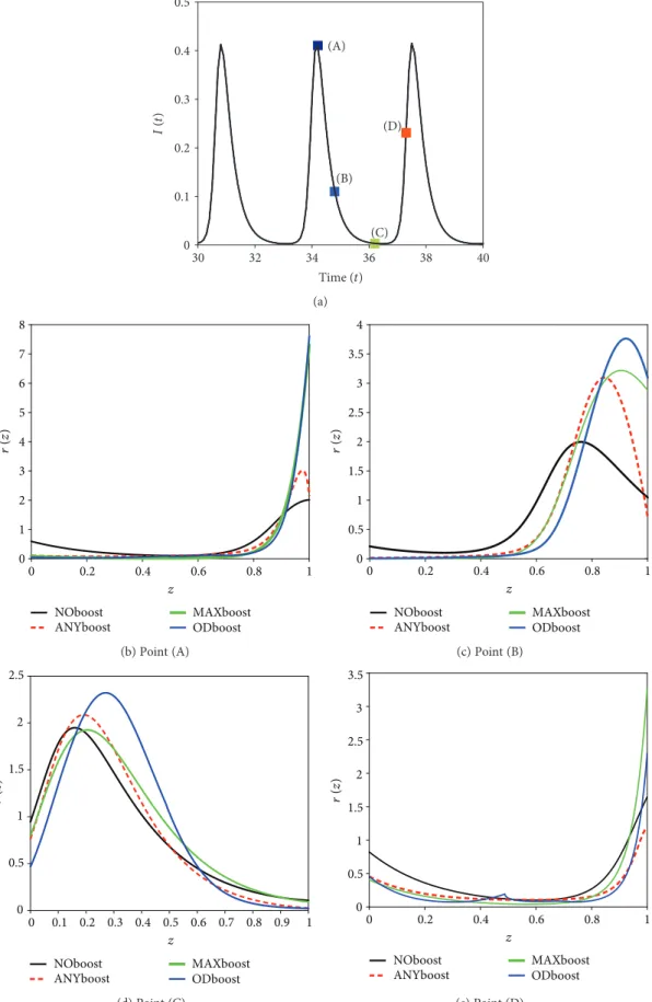
In Figure 10, we compare the immune distributionr t,z corresponding to different levels of an outbreak, for different boosting mechanisms. Figure 10(a) shows four points on a typical infective curve (I) which we shall consider for comparison. Point A corresponds to the infection peak, that is, the time point at which the infective population is at its maximal value. Point B and point D correspond to intermediate levels in the infective population, just after, respectively, just before an outbreak peak. Point C corresponds to the time point at which the infective population is at its minimal level. We see in Figures 10(b)–10(e) that the different immune responses yield qualitatively similar immune distributions with immunity waves moving from right to left. At the infective peak (Figure 10(b)), following primary infection and reexposure to the pathogen, most of

the population has a very high immune status (z∈ 0 8, 1) which slowly decays, reaching the level at which most of the population has a low to intermediate immune level (z∈ 0, 0 6) (Figure 10(d)). Just before a new outbreak, most of the hosts have very low (z∈ 0, 0 2) or very high (z∈ 0 8, 1) immunity (Figure 10(e)).

4. Conclusion

Understanding the role of immune system boosting due to the interplay of in-host and between hosts dynamics is a central point in immunoepidemiology of infectious diseases.

Employing the mathematical models (3), (4), and (5), in this work, we have systematically investigated the eﬀects of diﬀerent (in-host) immune responses at population level.

The boosting mechanisms studied here are in part taken or inspired by previous literature, for example, on measles [6, 13], pertussis [14], and inﬂuenza [15].

Our results indicate that the in-host immune response, that is, the individual boosting mechanism, has important eﬀects on the qualitative dynamics of the epidemics. The numerical results show that observing the distribution of immune level among recovered individuals, one can

3 2.5 2 1.5 1 0.5 030

20 10

0 0 0.2 0.4

Immunity level ( z) Time (

t)

r (t,z)

0.6 0.8 1 2.5 2 1.5 1 0.5

(a) NOboost

Time ( t)

Immunity level ( z)

r (t,z)

1.0 5

300

20 10

0 0 0.2 0.4 0.6 0.8 1 1 2 3 4 5 6 7 8

(b) MAXboost

5 4 3 2 1 400

30 20

10 0 0

0.5

1 0.5

1 1.5 2 2.5 3 3.5 4 4.5

t)

r (t,z)

(c) ANYboost

t)

r (t,z)

10 8 6 4 2 400

30 20

10 0 0

0.5

1 1

2 3 4 5 6 7 8

(d) ODboost

Figure8: Ther t,z solution for diﬀerent boosting mechanisms. (a) Waning immunity, absence of immune boosts. (b) Boost to maximal level of immunity. (c) Uniform probability of boosting to any higher immunity level. (d) Nonlinear boost according to Figure 3(c).

(10)

reconstruct the underlying boosting mechanism. When the trajectories of the systems (3), (4), and (5) approach an endemic equilibrium (Figure 4(b)), the distribution of immunity uniquely identiﬁes the boosting mechanism gov- erning the immune response in case of secondary infections.

Also for diseases with repeated outbreaks, it is possible to infer the immune boosting mechanism from the temporal evolution of immunity, though in this case, it is conve- nient to look at the dynamic of the immune population over time (Figures 8 and 9), rather than at the immune distribution (Figure 10).

This paper presents a novel mathematical study of temporal evolution of immune status in a population.

Despite the large number of publications in mathematical epidemiology or mathematical immunology, to the best of our knowledge, there have been only few authors who have eﬀectively combined in-host dynamics and processes at population level [6, 13, 16, 17], though only in [6, 13] the temporal evolution of immunity has been considered. If we

compare the stationary distribution of immunity of HKboost in Figure 4(b) with Figure 3(c) in [6], we observe that the results are rather diﬀerent, the curve in [6] being smoother.

We conjecture that the differences are on the one hand due to the choice of the parameters in the system, on the other hand to the different nature of the mathematical models. In [6], a large system of ordinary differential equation is presented, including exposed hosts and immune structure in all compartments, not only in the recovered ones as it is in our work. Here, we focused on a simple model for susceptible-infective-recovered dynamics in order to understand the role of immune boosting and waning immunity. We plan to extend the models (3), (4), and (5), by means of physiologically structured susceptible and exposed populations.

Parameter values used for all numerical simulations presented in this work are not inspired by a speciﬁc infectious disease, as we purely focused on the eﬀects of waning and boosting. Nevertheless, the model is suitable to describe

30

25

20

15

10

5

00 0.2 0.4

Immunity level (z)

Time (t)

0.6 0.8 1

0.5 1 1.5 2 2.5

(a) NOboost

Immunity level (z)

Time (t)

00 5 10 15 20 25 30

0.2 0.4 0.6 0.8 1 0

1 2 3 4 5 6 7 8

(b) MAXboost

40 4.5

4 3.5 3 2.5 2 1.5 1 0.5 35

30

20 25

15 10 5 0

Immunity level (z)

Time (t)

0 0.2 0.4 0.6 0.8 1

(c) ANYboost

Immunity level (z)

Time (t)

40 35 30 25 20 15 10 5

00 0.2 0.4 0.6 0.8 1 0

1 2 3 4 5 6 7 8

(d) ODboost

Figure9: Contour plot of thersolution for diﬀerent boosting mechanisms. (a) Waning immunity, no boosts. (b) Boost to maximal level of immunity. (c) Uniform probability of boosting to any higher immunity level. (d) Nonlinear boosting function as in Figure 3(c).

(11)

Time (t) 0

0.1 0.2 0.3 0.4 0.5

I (t)

(D) (A)

(B)

(C)

30 32 34 36 38 40

(a)

z 0

1 2 3 4 5 6 7 8

r (z)

NOboost

ANYboost MAXboost

ODboost

0 0.2 0.4 0.6 0.8 1

(b) Point (A)

z 0

0.5 1 1.5 2 2.5 3 3.5 4

r (z)

0 0.2 0.4 0.6 0.8 1

NOboost

ANYboost MAXboost

ODboost (c) Point (B)

z 0

0.5 1 1.5 2 2.5

r (z)

0 0.1 0.2 0.3 0.4 0.5 0.6 0.7 0.8 0.9 1 NOboost

ANYboost MAXboost

ODboost (d) Point (C)

0 0.2 0.4 0.6 0.8 1

z 0

0.5 1 1.5 2 2.5 3 3.5

r (z)

NOboost

ANYboost MAXboost

ODboost (e) Point (D)

Figure10: Comparison of immune distribution for diﬀerent boosting mechanisms at diﬀerent levels of an outbreak. (a) TheIsolution and the four reference points to be considered for comparison: (A) the infection peak, (B) an intermediate level after the outbreak, (C) the minimal infection level, and (D) just before a new outbreak. (b–e) Immune distribution corresponding to the points (A)–(D).

(12)

several infectious diseases, prior proper choice of the parameters. Certain studies, for example [5, 18], introduced a further parameter κto express a relative force of infection for reexposure, so they represent the rate of boosting by the term (κβI). This is reasonable if we think that during contacts, boosting occurs with a diﬀerent chance compared to primary infection. In this paper, we have assumed that the force of infection in secondary exposure is the same as in primary exposure (κ= 1).

The in-host dynamics described in this paper is rather coarse. The immune status of recovered individuals is represented by a single scalar quantity (z) which does not specifi- cally represent any kind of cells of the immune system. We are aware of the fact that the immune system is indeed very complex, and careful mathematical modeling should also take into consideration nonlinear in-host processes and interactions among the different players of the innate and adaptive immune system. Nevertheless, such afine descrip- tion would quickly lead to a complicated mathematical model, making it hard to achieve any reliable analytical or numerical result at population level.

A further limitation of the model is the assumption on the sharp threshold z_min, which defines the criterion for transition from immune to susceptible compartment. It is plausible that this transition does not occur in such an on- off manner, but it is rather a continuous process; that is, recovered individuals with a certain critically low level of immunity are less likely to get immune boost and more likely to experience a new infection, as suggested in [14]. Moreover, it is known that the immune system is differently reactive at different life stages, in particular immune boosts are weaker in children and elderly than in adults (see, e.g., the case of pertussis considered in [19]). We plan to extend the model including age heterogeneity.

Immune boosts occur not only after natural infection but also in case of vaccine-induced immunity. Current vaccination schedules include“boosters”whose goal is the prolonga- tion of protection against a certain pathogen [20]. The mathematical models (3), (4), and (5) can be extended to include vaccination and natural boosts induced in vaccinated hosts by contact with infectives (see [21]). Similar investiga- tion as proposed in this paper can be repeated in the context of vaccination.

Our results indicate that immune system boosts from natural secondary infections importantly aﬀect the immune dynamics at population level. We hope that ourﬁndings will stimulate future research in controlling infectious diseases via vaccination and vaccine design.

Data Availability

No data were used to support this study.

Conflicts of Interest

The authors declare that there are no conﬂicts of interest regarding the publication of this paper.

Acknowledgments

M. V. Barbarossa is supported by the European Social Fund and by the Ministry of Science, Research and the Arts Baden-Württemberg. The work of M. Polner was supported by the János Bolyai Research Scholarship of the Hungarian Academy of Sciences, the EU-funded Hungarian Grants EFOP-3.6.2-16-2017-00015 and NKFI KH 125628. G. Röst was supported by Marie Sklodowska-Curie Grant nos.

748193 and NKFI FK 124016.

References

[1] D. Wodarz,Killer Cell Dynamics: Mathematical and Computa- tional Approaches to Immunology, vol. 32, Springer, 2007.

[2] I. J. Amanna, N. E. Carlson, and M. K. Slifka,“Duration of humoral immunity to common viral and vaccine antigens,” The New England Journal of Medicine, vol. 357, no. 19, pp. 1903–1915, 2007.

[3] Z. Luo, H. Shi, H. Zhang et al.,“Plasmid DNA containing multiple CpG motifs triggers a strong immune response to hepatitis B surface antigen when combined with incomplete Freund’s adjuvant but not aluminum hydroxide,”Molecular Medicine Reports, vol. 6, no. 6, pp. 1309–1314, 2012.

[4] N. Arinaminpathy, J. S. Lavine, and B. T. Grenfell, “Self- boosting vaccines and their implications for herd immunity,” Proceedings of the National Academy of Sciences of the United States of America, vol. 109, no. 49, pp. 20154–20159, 2012.

[5] J. S. Lavine, A. A. King, and O. N. Bjørnstad,“Natural immune boosting in pertussis dynamics and the potential for long-term vaccine failure,” Proceedings of the National Academy of Sciences of the United States of America, vol. 108, no. 17, pp. 7259–7264, 2011.

[6] J. M. Heﬀernan and M. J. Keeling,“Implications of vaccination and waning immunity,” Proceedings of the Royal Society B:

Biological Sciences, vol. 276, no. 1664, pp. 2071–2080, 2009.

[7] M. V. Barbarossa, M. Polner, and G. Röst,“Stability switches induced by immune system boosting in an SIRS model with discrete and distributed delays,” SIAM Journal on Applied Mathematics, vol. 77, no. 3, pp. 905–923, 2017.

[8] M. V. Barbarossa and G. Röst,“Immuno-epidemiology of a population structured by immune status: a mathematical study of waning immunity and immune system boosting,”Journal of Mathematical Biology, vol. 71, no. 6-7, pp. 1737–1770, 2015.

[9] L. F. Shampine, “Solving hyperbolic PDEs in MATLAB,” Applied Numerical Analysis & Computational Mathematics, vol. 2, no. 3, pp. 346–358, 2005.

[10] R. J. LeVeque,Finite Diﬀerence Methods for Ordinary and Par- tial Diﬀerential Equations: Steady-State and Time-Dependent Problems, SIAM, Philadelphia, PA, USA, 2007.

[11] R. D. Richtmyer and K. W. Morton,Diﬀerence Methods for Initial-Value Problems, Wiley, New York, NY, USA, 1967.

[12] M. L. Taylor and T. W. Carr,“An SIR epidemic model with partial temporary immunity modeled with delay,”Journal of Mathematical Biology, vol. 59, no. 6, pp. 841–880, 2009.

[13] J. M. Heﬀernan and M. J. Keeling,“An in-host model of acute infection: measles as a case study,” Theoretical Population Biology, vol. 73, no. 1, pp. 134–147, 2008.

[14] W. F. de Graaf, M. E. E. Kretzschmar, P. F. M. Teunis, and O. Diekmann,“A two-phase within-host model for immune

(13)

response and its application to serological proﬁles of pertussis,” Epidemics, vol. 9, pp. 1–7, 2014.

[15] V. I. Zarnitsyna, J. Lavine, A. Ellebedy, R. Ahmed, and R. Antia, “Multi-epitope models explain how pre-existing antibodies aﬀect the generation of broadly protective responses to inﬂuenza,” PLoS Pathogens, vol. 12, no. 6, article e1005692, 2016.

[16] M. Martcheva and S. S. Pilyugin,“An epidemic model structured by host immunity,” Journal of Biological Systems, vol. 14, no. 2, pp. 185–203, 2006.

[17] L. J. White and G. F. Medley, “Microparasite population dynamics and continuous immunity,”Proceedings of the Royal Society B: Biological Sciences, vol. 265, no. 1409, pp. 1977– 1983, 1998.

[18] M. P. Daﬁlis, F. Frascoli, J. G. Wood, and J. M. McCaw,“The inﬂuence of increasing life expectancy on the dynamics of SIRS systems with immune boosting,” The ANZIAM Journal, vol. 54, no. 1-2, pp. 50–63, 2012.

[19] F. G. A. Versteegh, P. L. J. M. Mertens, H. E. de Melker, J. J.

Roord, J. F. P. Schellekens, and P. F. M. Teunis,“Age-speciﬁc long-term course of IgG antibodies to pertussis toxin after symptomatic infection withBordetella pertussis,”Epidemiology and Infection, vol. 133, no. 4, pp. 737–748, 2005.

[20] CDC,“General recommendations on immunization: recommendations of the advisory committee on immunization practices,” Morbidity and Mortality Weekly Report, vol. 60, no. 2, pp. 1–64, 2011.

[21] M. V. Barbarossa and G. Röst, “Mathematical models for vaccination, waning immunity and immune system boosting:

a general framework,”inBIOMAT 2014, R. P. Mondaini, Ed., pp. 185–205, World Scientiﬁc, 2015.

(14)

Hindawi

www.hindawi.com Volume 2018

Mathematics

^{Journal of}

Hindawi

Mathematical Problems in Engineering Applied Mathematics

Hindawi

Probability and Statistics

Hindawi

Mathematical PhysicsAdvances in

Complex Analysis

^{Journal of}

Hindawi

Optimization

^{Journal of}

Hindawi

Engineering Mathematics

International Journal of

Hindawi

Operations Research

Journal of

Hindawi

Function Spaces

Abstract and Applied Analysis

Hindawi

International Journal of Mathematics and Mathematical Sciences

Hindawi

Hindawi Publishing Corporation

http://www.hindawi.com Volume 2013

Hindawi www.hindawi.com

World Journal

Volume 2018

Hindawi

www.hindawi.com Volume 2018Volume 2018

Numerical Analysis Numerical Analysis Numerical Analysis Numerical Analysis Numerical Analysis Numerical Analysis Numerical Analysis Numerical Analysis Numerical Analysis Numerical Analysis Numerical Analysis

Numerical AnalysisAdvances inAdvances in Discrete Dynamics in Nature and Society

Hindawi

Hindawi www.hindawi.com

Differential Equations

Volume 2018 Hindawi