MEASURING HETEROGENEITY OF HOUSE PRICE DEVELOPMENTS IN HUNGARY, 1990–2016

(1)

MEASURING HETEROGENEITY OF HOUSE PRICE DEVELOPMENTS IN HUNGARY, 1990–2016

Ádám BANAI – Nikolett VÁGÓ – Sándor WINKLER

(Received: 15 May 2017; revision received: 19 January 2018;

accepted: 15 June 2018)

This study presents the detailed methodology of generating house price indices for the Hungarian market. The index family is an expansion of the Hungarian housing market statistics in several regards. The nationwide index is derived from a database starting from 1990, and thus the national index is regarded as the longest in comparison to the house price indices available so far. The long time series allow us to observe and compare the real levels of house prices across economic cycles.

Another important innovation of this index family is its ability to capture house developments by regions and settlement types, which sheds light on the strong regional heterogeneity underlying the Hungarian housing market.

Keywords: housing market, house price index, hedonic regression, Hungary JEL classifi cation indices: C430, R210, R310

Ádám Banai, Director at Magyar Nemzeti Bank (MNB, the central bank of Hungary).

E-mail: banaia@mnb.hu

Nikolett Vágó, corresponding author. Senior economist at Magyar Nemzeti Bank (MNB, the cen- tral bank of Hungary). E-mail: vagon@mnb.hu

Sándor Winkler, Senior economist at Magyar Nemzeti Bank (MNB, the central bank of Hungary).

E-mail: winklers@mnb.hu

(2)

1. INTRODUCTION AND MOTIVATION

Housing market is organically connected to every part of the economy and has a potentially large-scale impact on each area. As residential property is one of the most important assets of households, changes in house prices are likely to affect households’ consumption and saving decisions, while having a social aspect through affecting housing affordability. Similarly, the real estate market developments directly affect the business sector. Price developments and the number of transactions affect demand for the new investment projects and ultimately, the construction industry. Finally, developments in the real estate market also exert a direct impact on the banking sector. Changes in the prices of the real estate collaterals behind mortgage loans may not only determine the performance of the loans, but the recovery through the sale of collaterals in the event of default.

Beside the outstanding portfolio, an active real estate market boosts the demand for housing loans and affects the banking sector through a larger volume of new disbursements. Compared to the corporate loans, the banking sector can earn larger spreads on the mortgage loans, and the intensifying activity has a positive impact on profitability.

In addition to the factors described above, understanding the trends and identifying the risks arising in the real estate market are of key importance for the central banks. The house price index is designed to serve this particular purpose, providing insight into the processes in the real estate market and its individual segments.

In Hungarian practice, two indices have been in use so far: those published by FHB Bank and the Hungarian Central Statistical Office (HCSO). Although both indices provide a fair view of the domestic housing market developments, the construction of additional house price indices was necessary for Magyar Nemzeti Bank (MNB, the central bank of Hungary) from a financial stability perspective.

Having been available since 1998, the FHB index is typically published with a considerable lag (5–8 months) and it is constructed on the basis of a sample that covers only around 50 per cent of all transactions. The HCSO launched its own house price indices in 2007, with a primary focus on presenting the differences in the dynamics of new and used property prices.

Compared to these two indices, the MNB house price index family¹ presented in this study represents a step forward in several regards. (1) The index developed by the authors has been constructed on the longest and most comprehensive time

1 Hereinafter, we refer to the indices developed by the authors as ”MNB house price indices”, because these indices are used for exploring the house price trends and identifying the financial stability risks, while these are also the official statistical house price indices of the MNB.

(3)

series: it captures the developments of Hungarian house prices on a national scale starting from 1990. This is important because both the modelling of house prices and the assessment of housing market developments require the longest possible time series. (2) Starting from 2001, the index sheds light on the heterogeneity of house prices across regions and municipality types. By contrast, the previous indices provided an overall view of the country as a whole, only obscuring the different behaviour patterns of individual regions. From a business, banking and central banking perpektive, however, it is essential to be aware of housing market heterogeneitis between regions and municipality types. Even when the national price movements do not indicate any problems, individual regions can be exposed to potentially harmful developments. The extreme spikes in house prices or housing market bubbles typically arise in the capital cities or larger municipalities, which can be largely attributed to the central role of major cities in the economy and their more advanced infrastructural and institutional coverage.

In Section 2, we provide an overview of the traditionally applied methods in the construction of house price indices. Section 3 describes the transaction data on which the price indices are based. Section 4 is dedicated to the methodology used for the construction of our indices. In Section 5, we outline our regression results and present the derived house price indices. In Section 6, we conduct a robustness analysis for the methodology of the indices. Finally, Section 7 provides conclusions.

2. LITERATURE REVIEW

The calculation of changes in house prices aims to determine the average percentage change of residential property in a specific area during the review period. The actual market price of residential properties evolves during the sale and purchase of the properties; consequently, the housing market turnover provides a suitable basis for measuring the changes in house prices. Although the residential property prices can also be determined by appraisal, the comprehensive and regular appraisals of the stock of dwellings are scarce even by the international standards, primarily because of the high costs of data collection.² Consequently, the changes in house prices are typically computed from transaction prices.

Ideally, for the calculation of average price changes, each dwelling should change owners in each review period (e.g. year); only in that case would the market price data be available on each individual property. In reality, however,

2 House price indices in New Zealand, Denmark, the Netherlands and Sweden are constructed from stock appraisals.

(4)

only a fraction of the dwelling stock is sold in a given location in each period, and the diverging composition of the transactions executed in the given period poses problems. Since the dwellings sold may represent different types and quality in each period, changes in the average or median transaction prices do not reveal meaningful information about the average or typical change in the value of the total housing stock. In order to receive information explicitly about the price changes, we should observe the trading of the houses that have the same quality and attributes. The house price indices are essentially designed to achieve this goal: controlling for the quality traits of the dwellings, they capture the average

“pure” price change in the residential properties.

While computing the price index from transaction data, it should be borne in mind that despite controlling for the effect of diverging transaction composition of individual periods, the index remains susceptible to the types of dwelling traded in the given period and to the circumstances that certain locations are over-represented in the market turnover in a given country, relative to the dis- tribution of the total housing stock. The availability of detailed regular statistics on the composition of the housing stock may help eliminate this problem. Based on such statistics, new weights can be assigned to transaction data that are not representative of the overall housing stock. In the absence of such information, the evaluation of the indices derived from the transaction data should factor in the constraints mentioned above. Finally, it should be noted that statistical offices typically rely on transaction data in the compilation of house price indices; consequently, the above mentioned limitations are also present in the international house price statistics.

The main difference between the construction methods of house price indices arises from their treatments of the bias, stemming from the compositional shifts observed in the consecutive periods. In the following section, we provide an overview of the possible house price index calculation methods based on the classification presented in the handbook issued by Eurostat (2013), turning more attention to the hedonic regression methods used also for the house price indices of this study.

Hedonic regression models

The estimation of hedonic regression models is the most widely used method for calculating house price indices. The basic assumption of this approach is that the residential property prices can be determined as a function of their individual characteristics, and therefore the use of explanatory variables expressing the characteristics of the house under a linear regression model can control for the

(5)

bias arising from the composition effect. The technique of hedonic regression estimates dates back to Court (1939) and Griliches (1961), while the conceptual bases of the method were laid down by Lancaster (1966) and Rosen (1974). In Hungary several authors have alredy analyzed hedonic regression models on domestic data, Horváth (2007) compared the hedonic regression models with other methods on a sample of advertisement data for a homogenous residental area of the capital city of Hungary, Budapest. Horváth–Székely (2009) presented a house price index for used homes calculated by a hedonic regression modell on transaction data obtained from the tax authority. Kutasi–Badics (2016) compared a hedonic regression and an artifical neural network modell in terms of market price prediction for the Budapest market using a large set of advertisement data.

From the observations of price changes, the hedonic regression method at- tempts to strip out the composition effect arising from the trading of real properties with different characteristics across periods by including the following variables:

floor area of the structure, size of the land (for single detached dwelling units), the characteristics of its environment, age and type of the dwelling (e.g. detached house, row house, condominium, etc.), the materials used in the construction of the house, and the internal characteristics of the dwelling (e.g. number of bed- rooms and bathrooms, energy efficiency, etc.). The hedonic regression models are traditionally estimated by the method of ordinary least squares (OLS). Based on the time horizon of the estimate, three main types of hedonic modelling can be distinguished: the time dummy variable method, the adjacent-period approach and the multiperiod time dummy method.

In the case of the time dummy variable approach,³ a pooled OLS estimate is prepared based on the data of all periods. Except for the initial base period, the model uses separate dummy variables to capture price changes between each period as the price index is produced by exponentiating the time dummy coefficients. The regression equation can be written as:

0 1 1 2 2

2

,

T

i i i k ki t ti i

t

log y β β x β x β x δd ε



    



 ⁽¹⁾

where y is the price of the house, x denotes the characteristics of the house, d_t is the time dummy for period t, β expresses the coefficients of the control variables, δ_t means the coefficients of the time dummies and ε is the residual value. One po- tential drawback of this approach is that the coefficients of the model’s explanatory variables are constant over time, and if the characteristics of the property exert a different impact on the property price over time, the index will be subject to bias. Moreover, it might be problematic from a practical point of view that a

3 The model was originally developed by Court (1939).

(6)

new estimate must be prepared for the entire time horizon in each period; consequently, the entire time series of the price index will be subject to revision in each period.

Under the adjacent-period model, estimates are produced for the observations of two consecutive periods. In practice, this technique is a restricted form of the previously described time dummy variable method. If T means the number of all review periods, then a total of (T–1) estimates must be run in order to receive the price index. Since the estimation samples include the observations of two periods, each regression equation includes a single time dummy. The period-to- period price index can be computed by exponentiating the time dummy coefficients. The estimated regression for period t can be written as:

0 1 1 2 2

, ( 2, 3, , )

t t t t t t t t t t t

i i i k ki i i

log y β β x β x β x δ d ε t  T (2) where y is the price of the house, x denotes the characteristics of the house, d is the time dummy, β expresses the coefficients of the control variables, δ represents the coefficients of the time dummy and ε is the residual value. Since a separate estimate is produced for each adjacent-period pair, the greatest advantage of this method is that the estimated coefficients of the explanatory variables can change over time. Therefore, this method eliminates the underlying assumption of the time dummy variable model, i.e. the parameters are constant over time. This is consistent with the assumption that the demand and supply conditions can change over time with respect to the specific characteristics of the properties. Compared to the time dummy variable model, the downside of this approach is the far smaller sample size on which the estimate can be run. Consequently, this approach is only recommended if a sufficient number of observations are available for each adjacent-period pair. That notwithstanding, the method is considered to be advan- tageous from a statistical standpoint, as the previous elements of the time series are not subject to revisions again and again during the estimation of the additional index values.

In the multiperiod time dummy approach,⁴ the hedonic regression model must be estimated separately for each individual period. The calculation of the price index requires the definition of a “benchmark property”, and the house price index is defined as the price change of the benchmark property. For the computation of the pure price change, therefore, we need to determine the values of the property

4 This methodology was applied, among others, by Crone – Voith (1992), Knight et al. (1995), and Gatzlaff – Ling (1994); however, the authors used different terms to refer to this particular type of hedonic modelling.

(7)

characteristics included in the model. The regression equation for period t is the following:

0 1 1 2 2

logy_i^t  β^tβ^t x^t_iβ^tx^t_iβ_k^t , ( 2, 3, , )x^t_kiε_i^t t  T (3) where y is the price of the house, x denotes the characteristics of the house, β expresses the coefficients of the control variables, and ε is the residual value. This method should be preferred to the previously described approaches as the assumption is that the property characteristics captured by the explanatory variables of the model can change not only from half-year to half-year but also from quarter to quarter. It is problematic, however, that the definition of the “benchmark property” can be ambiguous (e.g. the typical property of the initial or the previous period), and the price index received largely depends on the benchmark property.

In many cases, the Fisher price index is used, which is defined as the geomet- ric average of the Laspeyres price index (which is computed from the average property characteristics of the base period) and the Paasche price index (which is weighted with the average property characteristics of the current period). Another disadvantage of this model is that its estimates may render even more uncertainty by the lack of sufficient observations for each period.

It should be noted that the risk of multicollinearity may arise in all three types of the hedonic models. A high correlation between the explanatory variables increases the standard errors of the coefficients, and some variables may become insignificant. Since the estimated coefficients, which are unbiased even in the event of multicollinearity, bear the most relevance for the house price index using as many variables as possible should be considered, hence reducing the risk of bias arising from the missing variables.

One possible extension of the methods drawing on hedonic regressions is the calculation of stratified indices. Sub-samples are separated according to some criteria relevant to the analysis (e.g. regions, municipality types). The hedonic models may be estimated for each individual sub-sample even according to different specifications, resulting in a separate sub-index for each sub-sample. With proper weighting, the sub-indices may aggregate up to a consistent house price index. One of the benefits of the approach is that the compilation of sub-indices supports the analysis of house prices separately for each sub-sample. In addition, since a separate estimate is prepared for each sub-sample and the coefficients of the explanatory variables may vary, we can factor in the fact that the characteristics of the reviewed properties included in the model may exert a different impact on the prices of the individual sub-samples. For the sake of reliability, each sub- sample should include a sufficient number of observations.

(8)

Other methods

The stratified sample mean method compiles the index based on average price changes computed within homogeneous groups that are created on the basis of various price determinant attributes. An aggregate house price index is built by taking the weighted average of the values computed for different groups/strata.

The advantages of the method are that it is easy to apply and explain to users, and that the sub-indices can be interpreted independently. As a significant drawback, however, it is difficult in practice to truly control for the composition effects mentioned above.

The repeat sales method was first proposed by Bailey et al. (1963). Besides the Federal Housing Finance Agency (FHFA), Standard & Poor (2009) compiles a house price index based on this method for 20 cities in the United States. This method only considers price changes in those properties that have been sold more than once over a specific time horizon. The main advantage of the model is the irrelevance of control variables in the estimate; the only bias that may arise is due to the depreciation of the dwelling units or their renovation induced appreciation.

The method can be applied efficiently if the sample of dwellings sold more than one time in the reviewed real estate market and period is high enough. Since the estimate covers the entire review period, the entire model must be re-estimated in each case, and therefore the price index is subject to revisions in each individual period. Beyond the models presented above, there are combined methods that use the hedonic regressions and the repeat sales method in conjunction with one another in order to maximise their benefits. In practice, however, such techniques are hardly used due to the complexity of the model and to the relatively minor observed improvement in efficiency.

The data requirements of the methodologies described above are different. The data available to us so far (presented in Section 3) are primarily suitable for the purposes of the hedonic regression models.

3. DATA

The changes in house prices can be statistically measured by using two types of data: (1) the value data of the stock of dwellings, or (2) the transaction data evolved during the sales and purchases of the properties. The former are typically derived from the real estate property appraisals. Internationally, there are only a handful of examples of data being regularly released on the value of residential properties pertaining to the total stock. The latter are traditionally collected by tax authorities in relation to property transactions. Therefore, statisticians tend to rely

(9)

on the transaction data for the compilation of house price indices. We compiled the house price indices based on the property acquisition duty data collected by the Hungarian National Tax and Customs Administration (NTCA).

Aside from the current demand and supply conditions, house prices are determined by attributes falling into two main groups: (1) the characteristics of the residential property itself, i.e. the quality of the property, and (2) the location of the property, i.e. the characteristics of its environment and location. The data collected by the NTCA include the most basic information related to the sales of the properties. In addition to the sale price, information is available on the property’s net internal area (NIA), the exact location and the type of the property (e.g. detached house or flat) and, starting from 2008, on whether the home is newly built or not. Information on the condition and qualitative characteristics of the residential properties is of insufficient quality and quantity. Overall, the data collected by the NTCA are mainly suitable for explaining the price of the properties with their NIA and location. With respect to the variables stored in the database, there are few differences⁵ in the data collected before and after 2008, which we addressed by defining different model specifications for before and after 2008.

For our purposes, we also retain those transactions in the database where the party acquiring the property is a business organisation. These observations make up only about 7 per cent of the post-2008 data. In addition, since the types of the residential properties changing hands in these cases are similar to those traded in the transactions of private individuals – i.e. they also constitute an integral part of the housing market turnover and the market itself – their inclusion in the estimate appears to be warranted.

With all unusable observations stripped out, the NTCA duty database currently contains information on around 3.1 million property transfers between 1990 and 2016 Q2. The variables of the database and the list of municipality-level variables linked to the database and included in the estimations are illustrated in Table 1.

Information on the NIA of the real estate is essential for determining the price of the properties. One of the greatest deficiencies of the database is the fact that in some cases, the value of the useful NIA is either incomplete or zero. In order to prevent the loss of an inordinate amount of data, this incomplete NIA data must be back-cast. The precise methodology of this exercise is explained in Subsec- tion 4.1. We need to stress that the Budapest sales data have only been available in the NTCA duty database from 2001, which should be borne in mind during the assessment of the pre-2001 house price index values.

As the NTCA database contains limited information on the characteristics of the dwellings, numerous location-dependent variables have been included in the

5 For a detailed description of the deficiencies in the data see Banai et al. (2017).

(10)

Table 1. Definition of the dataset and the individual variables used in the estimation

Source Variable Description

NTCA duty database

Price (ln) (HUF)

The price of the real estate is the dependent variable of the regressions. It is the larger among National Tax Authority’s valuation and the price in the transaction contract. The variable is in a logarithmic form.

Quarter Quarter of property acquisition duty.

Type of property * Size of property (ln)

The net internal area (NIA) is in the regressions by categories of the type of dwelling.

The category variable “type of dwelling” can have the following values: family house in inner and outer districts (in the case of Bp.), family house in county seat and other cities (in the case of cities), condominium, panel block of flats and homestead. In case of data before 2008 there are only two categories:

family house and flat.

New flat Category variable: new or used property.

Variables based on the HCSO id of the settlement

Districts Category variable: districts of Budapest.

Agglomeration

Category variable: 8 districts distinguished:

agglomeration of Szeged, Pécs, Debrecen, Miskolc, Székesfehérvár, Budapest, Győr and Sopron.

Recreational area

Category variable: 7 seasonal property areas distinguished: Lake Balaton - near shore, Lake Balaton - other, Dunakanyar, Mátra-Bükk, Sopron-Kőszeghegyalja, Lake Tisza, Lake Velence - Vértes.

County Category variable: county of the settlement.

TSTAR database

Population (ln) Population at the end of the year. The variable is in a logarithmic form.

Size (ln) Size of the municipality. The variable is in a logarithmic form.

Local home support (ln)

(HUF) Amount of local housing subsidies. The variable is in a logarithmic form.

Geox database

Distance from Budapest (ln) The shortest distance from Budapest expressed in minutes. The variable is in a logarithmic form.

Distance from county seats (ln)

The shortest distance from the county seat expressed in minutes. The variable is in a logarithmic form.

NTCA PIT

database Total income per capita (ln)

(HUF) Net labour income per capita. The variable is in a logarithmic form.

Note: The Geox database contains the location of Hungarian municipalities relative to specific nodes and cen- tres (e.g. distance from Budapest or from the nearest highway node). The distances are expressed both in time and kilometres. The TSAR database is maintained by the HCSO and contains comprehensive information on Hungarian municipalities (e.g. demography, institutional coverage, tourism, etc.). Inner districts in the Budapest model: I, II, III, V, VI, VII, VIII, IX, XI, XII, XIII, and XIV.

(11)

data used for the compilation of our index. We selected these explanatory variables based on two main criteria: on the one hand, we tried to include the variables that did not correlate strongly; on the other hand, in selecting the variables we fo- cused on indicators that may carry significant additional house price information compared to the rest of the control variables. In addition, we obviously wanted to be certain that the sign of the explanatory variables included in the models is economically intuitive.

The location of the property can influence the sale price significantly. Larger municipalities, regional centres or the centres of smaller geographical units typically have better infrastructural and institutional coverage, and such factors may increase the appeal of these municipalities and, hence, the housing market of the area drives up the local house prices. Another important factor in the assessment of a residential property is its temporal distance from geographically key locations and nodes or whether it is located in municipal agglomerations or seasonal property areas. Smaller municipalities located closer to motorways with easy access to larger municipalities are more attractive than hard-to-access locations.

Additionally, we use the size (km²) and population of the municipalities, the total amount of local housing subsidies and the net per capita income of the municipalities for the modelling of house prices. The descriptive statistics of the data used for the estimation of the house price indices are included in the Annex (Table 6).

4. THE METHODOLOGY OF THE MNB’S HOUSE PRICE INDEX

4.1. The backcasting of useful NIA

One of the deficiencies of the database is the insufficient information available on the NIA of the residential properties. Depending on the period, data are una- vailable for around 30–40 per cent of transactions. The database also includes a variable referred to as the “property area” with a far higher, nearly 100 per cent availability; however, as to whether this information pertains to the area of the structure or to the plot of land varies for each observation and cannot be explicitly determined. We supply the missing values of the “useful NIA” variable from the appropriate values of the “property area” variable, and backcast the missing values with a regression method. In brief, we use the following method for the definition of the NIA:⁶

6 This procedure is consistent with the HCSO’s treatment of incomplete or incorrect NIA values; the two methods differ from one another only in respect of the details of the regression estimate.

(12)

1. We considered all “useful NIA” data under 15m² and over 500m² to be missing parameters.

2. Wherever the “useful NIA” is specified as “missing” or zero and the “property area” is under 150m², we consider the “property area” to be the “NIA”.

3. For observations where the “NIA” remains “missing” or zero even after the first two steps, we use a regression method to backcast the size of the

“NIA”.

Table 2 indicates the percentages of the observations by municipality type that must have been backcasted with the assistance of the linear regression method described in Section 3. Evidently, the missing NIA information mainly affects villages.

Table 2. Percentages of missing useful NIA information by year and by municipality type, %

Budapest Cities Villages Total

1990–2007 4.2 20.3 53.4 25.0

2008–2015 7.4 25.6 63.1 28.7

We used the ordinary least squares method to estimate the linear regression model fit to the logarithm of the NIA variable. We prepared an estimate for each municipality type (Budapest, cities and villages) both for the pre-2008 and post- 2008 samples. We divided the database into sub-samples representing the old and the new structures in order to use the broadest possible information base for both of these periods, while breaking down the backcasting by municipality types was warranted by the significantly diverging distributions of property size in the individual municipality types.

4.2. Methodology of outlier fi ltering

The linear regression models can be sensitive to the outliers⁷ in the database.

Firstly, the database might contain observations that are most likely incorrect, for example, owing to measurement or recording errors. Secondly, although some outliers may reflect existing processes, we should consider discarding them from the sample anyway, as they may significantly distort the estimate and the resulting price change. This underpins the significance of outlier filtering; indeed, discarding the extreme and influential data points may improve the accuracy of the regression estimate and the reliability of the conclusions drawn from the results.

7 Zrínyi et al. (2012) cite numerous outlier definitions from the academic literature.

(13)

With that in mind, we opted for a multi-step outlier filtering technique. In the first step, we tried to strip out the incorrect data points by defining absolute bounds for the main variables of the duty database (adjusted for the consumer price index for each year in the case of price-type variables). Observations were removed from the estimation sample if:⁸

 the sale price was lower than HUF 100,000 or higher than HUF 1 billion;

 the NIA of the dwelling was smaller than 15m² or larger than 500m²;

 the unit sale price per square metre was below HUF 2,000 or above HUF 10 million.

In the second step, we also performed filtering for statistical purposes. We estimated a regression equation (1) for the house price on the data points that were deemed correct based on the first step, and calculated the following four indicators to identify outliers and influential values:

1. Externally studentized residuals⁹:

 

( ) ,

(1 ),

i i

i

i ii

y y

r MSE h

 





where y_i is the observed price for the ith observation, y is the estimated value for ͡ _i

the ith observation, _{( )} ²

1

1 ⁿ ( ),

i i i

i

MSE y y

n _





^ is the mean squared error excluding the ith observation and h_ii is the leverage.¹⁰

For each observation, the indicator examines the standard error adjusted value of the estimated residuals (deviation between observed and estimated values).

The computed residuals are not homoscedastic (their variance is different), and the observations with the greatest leverage have residuals with the smallest variance, which is addressed by the 1h_ii term in the formula. The mean squared error included in the indicator is derived from a regression that does not include the reviewed ith observation. This is useful because the price estimate will be defined on the basis of the coefficients that are not skewed by the ith observation

8 The values provided for the sale and the unit price refer to 2015 Q4; thresholds for all other periods are received after adjustment for the consumer price index.

9 The indicator of externally studentized residuals is explained in detail by Belsley et al. (1980), Vellemen – Welsch (1981), Chatterjee – Hadi (1986), and Bollen – Jackman (1990).

10 Leverage is a measure of how far a data point deviates from the mean of the explanatory variables. In other words, it is a diagonal element of the hat matrix that shows the leverage exerted by the ith observed price (yi) on the ith estimated value (yi).

(14)

even if it is deemed to be an outlier; consequently, the indicator will not mistaken- ly yield price observations and price estimates that are too close to each other.¹¹ 2. Cook’s distance¹²:

2

( ) ( )

( )

1 (1 ) 1

i i ii i

i

i ii ii

y y h MSE

CD MSE h h MSE p

  

 

   

 

 

where y_i is the estimated price for the ith observation, y_(i) is the estimated value for the ith observation calculated from the coefficients of a regression obtained after the removal of the ith observation, p is the number of explanatory variables in the regression, MSE is the mean squared error, MSE_(i) is the mean squared error obtained after the removal of the ith observation and h_ii is the leverage of the ith observation.

As opposed to the studentized residual indicator that concentrates on the residual values, this indicator focuses on the dependent variable estimates obtained with and without the ith observation. In addition to the dependent variable, the effect of explanatory variables appears indirectly in the calculation through the leverage. A high value of the indicator suggests that the observation has a significant effect on the size of the estimated regression coefficients.

3. Welsch distance¹³:

( ) ( )

( 1) (1 ) 1

i i ii

i

i ii ii

y y h n

WD MSE h h

 

  

 

where y_i is the estimated price for the ith observation, y_(i) is the estimated value for the ith observation calculated from the coefficients of a regression obtained after the removal of the ith observation, n is the number of elements in the sample, MSE_(i) is the mean squared error obtained after the removal of the ith observation and h_ii is the leverage of the ith observation.

Similar to the previous indicator, this indicator measures the effect of the given observation on the estimated values; however, it uses a different normalisation and is more sensitive to the observations with high leverage. With similar outliers in the database, this indicator could be more efficient in identifying observations that are to be discarded.

11 It should be borne in mind that with several similar outliers in the database, the regression received after the removal of individual observations may be very similar to the regression that includes all of the observations.

12 For more detail, see Cook (1977), Hair et al. (1995) or Bollen – Jackman (1990).

13 For more detail, see Welsch (1982) or Chatterjee – Hadi (1986).

(15)

4. DFBETA¹⁴:

 

( )

( ' ) 1

j j i

ij

i jj

b b

DFBETA

MSE ^

 

X X

where b_j is the jth element of the vector of the coefficients, b_j(i) is the jth element of the regression that results when the ith observation is removed, MSE_(i) is the mean squared error computed after the removal of the ith observation and X is the matrix of the explanatory variables included in the linear regression model.

The indicator measures the sensitivity of the coefficients (deviation adjusted for variance) estimated with and without the ith observation for a randomly selected explanatory variable. Since the period’s dummy coefficient bears most relevance to the price index in the case of adjacent-period estimates, one of the benefits of the indicator is its ability to specifically measure the effect of the given observation on this particular coefficient.

In selecting the indicators, we tried to limit the overlaps between them to the minimum. According to the literature, based on the sample size and the number of the explanatory variables, each indicator can be used to identify the values that can be considered as outliers or influential based on the specific indicator. An observation will be included in the final estimation sample if it is deemed valid by at least 3 of the 4 above mentioned indicators.¹⁵ The results confirm that the selected indicators offer significant additional information relative to each other.

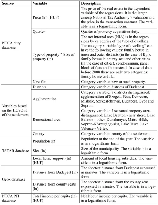
We identified the percentage of the observations that should be filtered out in the two steps, both for regions and for municipality types. As a result, we initially removed about 1 per cent of the observations from the estimation sample and in the second step 4–5 per cent of the observations were dismissed.

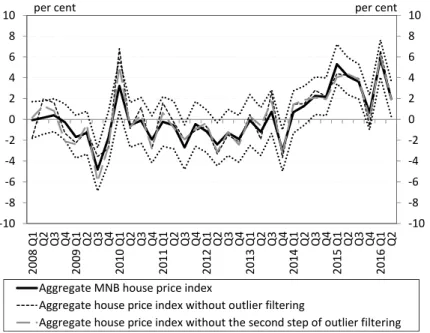
The effect of the filtering performed in the individual steps on the aggregate index is illustrated by Figure 1. We found that despite the far smaller number of observations excluded in the first step, these observations exert a far greater impact on the price index than those removed from the estimation sample in the second step. This is because in the first step we strip out obviously incorrect data points at the outer edge of the distributions.

4.3. Methodology of regression estimation

In consideration of the characteristics of the available database and the advantages and disadvantages of the specific methodologies as described in Subsection 3.1,

14 For more detail, see Belsley et al. (1980) or Bollen – Jackman (1990).

15 We performed a robustness analysis for this criterion, which is discussed in Section 6.

(16)

the estimation of a hedonic regression model for adjacent periods appears to be the most appropriate method. We prefer the adjacent-period estimate to the multiperiod time dummy method because one of our key objectives was to exam- ine the diverging characteristics of the individual municipalities and the regional processes separately. For this exercise, we need to divide the database into sub- samples, but the number of observations in the sub-samples are insufficient to run a reliable estimate for each individual period.

The adjacent pair estimation procedure has numerous advantages over the time dummy variable approach. On the one hand, as a result of estimating a separate regression equation for each adjacent-period pair, the partial effects exerted on the house price by the model’s control variables capturing the characteristics of the dwelling can be different over time, which is a more flexible approach and a better fit to economic intuition compared to the assumption of fixed effects irrespective of the periods. On the other hand, with the adjacent-period estimate we can compile a consistent house price index for the longest possible time horizon,

Figure 1. Nationwide MNB house price index with various outlier filtering procedures (quarterly changes)

Note: The black dotted line indicates the 95 per cent confidence interval* of the MNB’s aggregate house price index.

* The confidence interval of the aggregate national index was produced by weighting the 95 per cent confidence intervals of the quarter dummy parameters included in the models for individual municipality types with transactions.

Ͳ10 Ͳ8 Ͳ6 Ͳ4 Ͳ2 0 2 4 6 8 10

2008

Q1 Q2 Q3 Q4

2009

Q1 Q2 Q3 Q4

2010

Q1 Q2 Q3 Q4

2011

Q1 Q2 Q3 Q4

2012

Q1 Q2 Q3 Q4

2013

Q1 Q2 Q3 Q4

2014

Q1 Q2 Q3 Q4

2015

Q1 Q2 Q3 Q4

2016

Q1 Q2 percent percent

AggregateMNBhousepriceindex

Aggregatehousepriceindexwithoutoutlierfiltering

Aggregatehousepriceindexwithoutthesecondstepofoutlierfiltering

(17)

while using the broadest possible information base for all periods. An estimation for the entire period would entail a loss of information: it is the specificity of our database that there is less information available on each transactions until 2008, which would restrict the range of explanatory variables in the models from 2008.

It is another important factor that the national index estimated for the pre-2001 period (for which no sub-indices can be produced due to the insufficient number of transactions) can be consistently added to the national index compiled with the adjacent-period method for the period between 2001 and 2016 from the sub- indices created for each region and municipality type. This would not have been possible using the time dummy variable approach. Finally, the time series resulting from the adjacent-period estimate is not subject to revisions for methodologi- cal reasons¹⁶ with the release of new data.

4.4. Disaggregated indices

After cleaning the database, we divided it into sub-samples based on the legal sta- tus and region of the municipalities, and conducted the adjacent-period hedonic regressions separately for each sub-sample. According to the settlement types, we produced indices for Budapest, cities and villages. We defined the regional de- composition based on the number of observations available. As a result, we compiled 7 region-level city indices and produced the national house price indices for cities by weighting the city indices with the number of transactions. In the case of villages, the low number of observations prevented us from preparing reliable estimates for each region, and consequently, we do not compile the regional price indices for villages. Similar weights based upon the number of transactions are applied to receive the national quarterly price change from the quarterly price changes of homes in Budapest, cities and villages. Finally, we construct the aggregate house price index by chaining the previously received quarterly indices.

Since the number of real estate market transactions was significantly lower in the 1990s in Hungary, it was only from 2001 that the 9 disaggregated house price indices described above could be produced reliably. However, the adjacent-period estimate allows us to link the national-level quarterly price changes derived from the adjacent-period models for the period of 1990–2001 to the national aggregate index resulting from the weighting of the previously described disaggregated indices.

16 Irrespective of the estimation methodology, the values of the house price index are routinely subject to revisions because a certain part of the property transaction data used for the calculations are made available with a significant lag.

(18)

5. PRESENTATION OF THE RESULTS OF THE MNB’S HOUSE PRICE INDEX

5.1. Time series of the MNB’s house price index

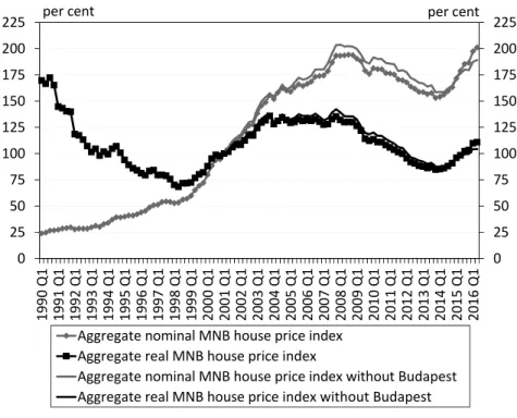
In this section, we present the house price indices estimated for the individual sub-samples and the MNB’s aggregate house price index. Because of the limitations of our database described above, for the period before 2001 we constructed only a national index, while indices decomposed by the settlement types and regions (for cities) start from 2001. Figure 2 illustrates the MNB’s aggregate nominal and real house price indices on a long time series. Since the database does not contain observations on transactions executed in Budapest before 2001, an aggregate house price index for the period after 2001 was estimated without taking into account the observations on residential properties located in Buda- pest. There is a significant difference between the two nominal time series only after 2014, which suggests that the house price dynamics before 2001 is properly described by the aggregated MNB house price index without Budapest.

Figure 2. Nominal and real MNB house price index (2001 Q1 = 100%)

Note: The real index is deflated with the consumer price index. Based on a national estimation until 2001 and aggregate from the sub-indices from 2001. The current MNB house price index values are available for down- load at the following link: http://www.mnb.hu/letoltes/mnb-lakasarindex.xlsx

0 25 50 75 100 125 150 175 200 225

1990Q1 1991Q1 1992Q1 1993Q1 1994Q1 1995Q1 1996Q1 1997Q1 1998Q1 1999Q1 2000Q1 2001Q1 2002Q1 2003Q1 2004Q1 2005Q1 2006Q1 2007Q1 2008Q1 2009Q1 2010Q1 2011Q1 2012Q1 2013Q1 2014Q1 2015Q1 2016Q1

percent percent

AggregatenominalMNBhousepriceindex AggregaterealMNBhousepriceindex

AggregatenominalMNBhousepriceindexwithoutBudapest AggregaterealMNBhousepriceindexwithoutBudapest

(19)

According to our calculations, between 1990 and 2007 the house price indices grew continuously in a nominal sense, but at varying rates in different phases.

Prices increased at a relatively slower rate between 1990 and 1999; during these years the house price level roughly doubled. The increase between 1999 and mid- 2003, however, is even more robust, in this four and a half years the prices rose by nearly 157 per cent. Although prices continued to increase until the 2008 crisis, the growth rate was far less pronounced. Based on the results of the MNB’s indices and consistent with the HCSO’s calculations, Hungarian house prices em- barked on a continuous decline that lasted until 2014. From the upswing in early 2014 house prices started to grow dynamically once again.

By 2016, the nominal level of house prices rose to a historical peak. After the sharp rise of the past two and a half years, on average, prices have already ex- ceeded the previous “peak” of 2007–2008. In real terms, however, house prices still fall significantly behind the levels recorded in 2003–2008.

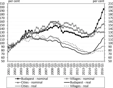
Broken down by regions and settlement types, the house price indices indicate a considerable heterogeneity in the Hungarian housing market. Budapest has witnessed more dynamic price increases in recent years than those seen in municipalities outside of the capital (Figure 3), while differences are also evident

Figure 3. The MNB’s nominal and real house price index by municipality typs (2002 = 100%)

50 60 70 80 90 100 110 120 130 140 150 160 170 180 190 200 210

2001

Q1 Q3

2002

Q1 Q3

2003

Q1 Q3

2004

Q1 Q3

2005

Q1 Q3

2006

Q1 Q3

2007

Q1 Q3

2008

Q1 Q3

2009

Q1 Q3

2010

Q1 Q3

2011

Q1 Q3

2012

Q1 Q3

2013

Q1 Q3

2014

Q1 Q3

2015

Q1 Q3

2016Q1

percent percent

BudapestͲnominal VillagesͲnominal

CitiesͲnominal BudapestͲreal

CitiesͲreal VillagesͲreal

(20)

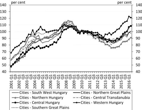
between certain regions (Figure 4). After 2008, the house prices did not exhibit such a steep downward shift in Western Hungary as in the rest of the country, while the house price levels in Northern Hungary, for example, fall far behind.

One important result of the regional breakdown of the house price index, overall, is the separate presentation of the house price changes in Budapest. In the current cycle, the pick-up in the housing market is strongly Budapest-oriented, which is well reflected in the 65 per cent nominal increase in the Budapest house prices between 2013 Q4 and 2016 Q2, compared to the national average of 31 per cent.

The sharp increase in the Budapest house prices, however, appears to be less re- markable once we consider that prices did not reach the 2008 level until 2016 in real terms (Figure 3).

5.2. Regression results

Regressions for Budapest, cities and villages are described separately. Due to the limited scope of this study, we only present the Southern Transdanubian region for the city indices constructed for the individual regions, because this region

Figure 4. The MNB’s nominal house price index for cities by regions (2010 = 100%) 40 50 60 70 80 90 100 110 120 130 140

40 50 60 70 80 90 100 110 120 130 140

2001

Q1 Q3

2002

Q1 Q3

2003

Q1 Q3

2004

Q1 Q3

2005

Q1 Q3

2006

Q1 Q3

2007

Q1 Q3

2008

Q1 Q3

2009

Q1 Q3

2010

Q1 Q3

2011

Q1 Q3

2012

Q1 Q3

2013

Q1 Q3

2014

Q1 Q3

2015

Q1 Q3

2016Q1

percent percent

CitiesͲSouthWestHungary CitiesͲNorthernGreatPlains CitiesͲNorthernHungary CitiesͲCentralTransdanubia CitiesͲCentralHungary CitiesͲWesternHungary CitiesͲSouthernGreatPlains

(21)

aptly illustrates the effect of the Balaton, the most important tourism catchment area apart from the Budapest agglomeration. Since the regression model is estimated over and over again for each quarter pair, of all the results we only present the regression results of the estimates required for the construction of the 2015 Q4 index.

Table 3 shows the regression outputs of the Budapest model. Estimated on a sample covering 2015 Q3 and 2015 Q4, the model has 69 per cent explanatory power.¹⁷ The dummy variable denoting 2015 Q4 shows that a Budapest transac-

17 It should be noted that the backcasting of the data improves the explanatory power of the regressions artificially.

Table 3. Regression results of the Budapest house price index model for 2015 Q4

Variables Variables

Quarter 2015 Q4 (ref.: 2015 Q3) 0.0278*** Districts (ref.: 1)

(0.0042) 2 0.0361*

New flat (ref.: used flat) 0.3507*** (0.0197)

(0.0162) 3 –0.3261***

Type of property * size of property (ln) (0.0187)

Condominium 1.2556*** 4 –0.4888***

(0.0767) (0.0194)

Panel block of flats 1.4491*** 5 0.2110***

(0.0819) (0.0214)

Family house (inner city) 1.0233*** 6 –0.1000***

(0.0718) (0.0198)

Family house (outer city) 1.1667*** 7 –0.2811***

(0.0692) (0.0190)

Type of property * size of property(ln)² 8 –0.4511***

Condominium –0.0416*** (0.0188)

(0.0097) 9 –0.2544***

Panel block of flats –0.0954*** (0.0196)

(0.0117) 10 –0.6225***

Family house (inner city) 0.0124 (0.0197)

(0.0095) 11 –0.1284***

Family house (outer city) –0.0265*** (0.0185)

(0.0083) 12 –0.0038

Constant 12.5399*** (0.0205)

(0.1524) Further categories

Number of observations 23386

Adj. R-squared 0.6867

Note: “ref.” indicates reference category. “Further categories” indicate that the regression table does not include all categories of the variable because of the lack of space, for the complete version see Banai et al. (2017).

Standard errors in brakets. *, **, *** indicates a coefficient significant at the 0.01, 0.05 and 1% level.

(22)

tion took place in 2015 Q4 as opposed to 2015 Q3, increased the price by e^0.0278 = 1.028; in other words, in 2015 Q4 the pure price change in the Budapest housing market was 2.8 per cent.

The NIA variable is included in the regression in its interaction with the type of the property; in other words, a 1 per cent increase in NIA may generate different price increasing effects for different property types. In addition to the linear term, the squared term of the NIA variable was also included in the models because in our view, a 1 per cent increase in useful NIA may have a different price increasing effect in the case of larger dwellings. Because of the inclusion of the squared term, the partial effect exerted by a 1 per cent difference in NIA depends on the size of the NIA; consequently, the examination of the estimated coefficients alone

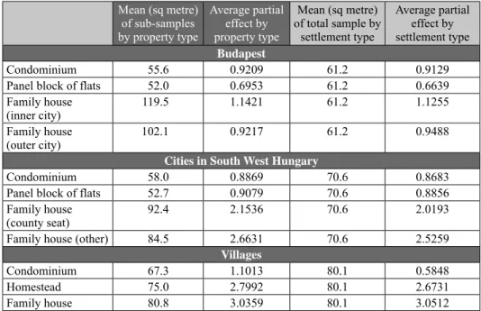
is not appropriate. For the model specified for Budapest, Figure 8 in the Annex illustrates the combined partial effect of the linear and squared terms on the price by property type. Table 4, in turn, indicates the average partial effects.

Evidently, a 1 per cent increase in NIA has the greatest positive impact on the value of detached houses. Moreover, the regression results show that the partial effect of NIA is significantly higher in the case of detached homes in the inner

Table 4. Combined partial effect of the linear and squared terms of the NIA variable by average NIA Mean (sq metre)

of sub-samples by property type

Average partial effect by property type

Mean (sq metre) of total sample by

settlement type

Average partial effect by settlement type Budapest

Condominium 55.6 0.9209 61.2 0.9129

Panel block of flats 52.0 0.6953 61.2 0.6639

Family house

(inner city) 119.5 1.1421 61.2 1.1255

Family house

(outer city) 102.1 0.9217 61.2 0.9488

Cities in South West Hungary

Condominium 58.0 0.8869 70.6 0.8683

Panel block of flats 52.7 0.9079 70.6 0.8856

Family house

(county seat) 92.4 2.1536 70.6 2.0193

Family house (other) 84.5 2.6631 70.6 2.5259

Villages

Condominium 67.3 1.1013 80.1 0.5848

Homestead 75.0 2.7992 80.1 2.6731

Family house 80.8 3.0359 80.1 3.0512

(23)

districts¹⁸ of Budapest compared to those located in the outer districts. In addition, with respect to the price effect of the NIA, there is a significant difference between brick homes and panel buildings: the partial price increasing effect of the NIA is greater for brick houses, which are considered to be of better quality.

Another interesting result from the regressions for Budapest is the fact that compared to the I. district, only the V. district has a price increasing effect; and in the rest of the districts, the residential properties tend to be cheaper on average. It is another intuitive result that the new residential properties are, ceteris paribus, more expensive on average.

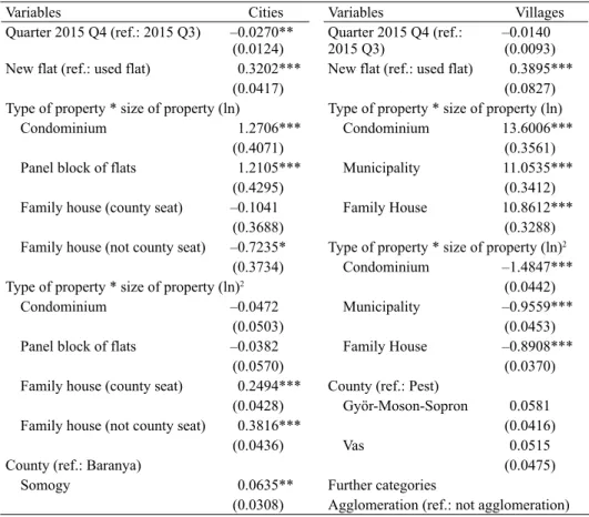
Table 5 depicts the regression results of the model constructed for Southern Transdanubian cities, also run on a sample of 2015 Q3 and 2015 Q4 transactions.

18 Inner districts featured in the model: I, II, III, V, VI, VII, VIII, IX, XI, XII, XIII, and XIV.

Table 5. Regression results of the villages and the Southern Transdanubian cities’ house price index model for 2015 Q4

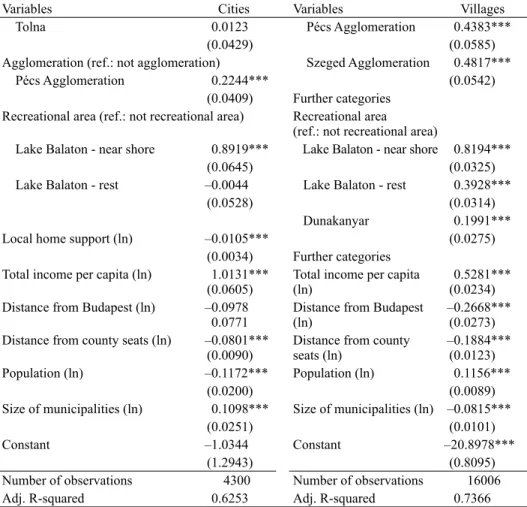
Variables Cities Variables Villages

Quarter 2015 Q4 (ref.: 2015 Q3) –0.0270**

(0.0124) Quarter 2015 Q4 (ref.:

2015 Q3) –0.0140

(0.0093) New flat (ref.: used flat) 0.3202*** New flat (ref.: used flat) 0.3895***

(0.0417) (0.0827)

Type of property * size of property (ln) Type of property * size of property (ln)

Condominium 1.2706*** Condominium 13.6006***

(0.4071) (0.3561)

Panel block of flats 1.2105*** Municipality 11.0535***