Unified approach of primal-dual interior-point algorithms for a new class of AET functions

C

U

B

Illés Tibor and Rigó Petra Renáta and Török Roland

Unified approach of

primal-dual interior-point algorithms for a new class of AET functions

http://unipub.lib.uni-corvinus.hu/7197

C

E

W

P

02/2022

UNIFIED APPROACH OF PRIMAL-DUAL INTERIOR-POINT ALGORITHMS FOR A NEW CLASS OF AET FUNCTIONS

TIBOR ILLÉS¹, PETRA RENÁTA RIGÓ^1,∗, ROLAND TÖRÖK²

1Corvinus Center for Operations Research at Corvinus Institute for Advanced Studies, Corvinus University of Budapest, Hungary;

2Doctoral School of Economics, Business and Informatics, Corvinus University of Budapest

18.02.2022.

Abstract. We propose new short-step interior-point algorithms (IPAs) for solvingP∗(κ)-linear complementarity problems (LCPs). In order to define the search directions we use the algebraic equivalent transformation technique (AET) of the system which characterizes the central path.

A novelty of the paper is that we introduce a new class of AET functions. We present the complexity analysis of the IPAs that use this general class of functions in the AET technique.

Furthermore, we also deal with a special case, namely ϕ(t) =t²−t+√

t. This function differs from the ones used in the literature in the sense that it has inflection point. It does not belong to the class of concave functions determined by Haddou et al. [24]. Furthermore, the kernel function corresponding to this AET function is neither eligible nor self-regular kernel function.

We prove that the IPAs using any memberϕof the new class of AET functions have polynomial iteration complexity in the size of the problem, bit length of the integral data and in the param- eter κ. Beside this, we also provide numerical results that show the efficiency of the introduced methods.

JEL code: C61

Keywords. Interior-point algorithm;P∗(κ)- linear complementarity problems; algebraic equiv- alent transformation technique; new class of AET functions

1. Introduction

Linear complementarity problems have been extensively studied nowadays. Linear pro- gramming (LP) and linearly constrained (convex) quadratic programming (QP) problems are special cases of LCPs. Several applications of LCPs arise in different fields, such as engineering, computational mechanics, game theory, economics, see [11, 21]. It was shown that solvability of LCPs related to quitting games ensures the existence of different ε-equilibrium solutions, see [40]. Bimatrix games can be also formulated as LCPs, see [33]. The Arrow-Debreu competitive market equilibrium problem with linear and Leon- tief utility functions can be transformed to LCP [46]. For detailed study on LCPs see the books of Cottle et al. [11] and Kojima et al. [31]. In the book of Kojima et al. [31] the theory of interior-point algorithms for solving LCPs is highlighted.

LCPs belong to the class of NP-complete problems, see [10]. However, the properties of the problem’s matrix have influence on the solvability of the LCPs. It is known that if the problem’s matrix is skew-symmetric [39,44,45] or positive semidefinite [32], IPAs can find approximate solution of LCPs in polynomial time. Cottle, Pang, and Venkateswaran

∗Corresponding Author.

E-mail addresses: tibor.illes@uni-corvinus.hu (Tibor Illés), petra.rigo@uni-corvinus.hu (Petra Renáta Rigó), roland.torok@stud.uni-corvinus.hu (Roland Török).

[12] introduced the class of sufficient matrices. The class ofP_∗(κ)-matrices was proposed by Kojima et al. [31]. If we consider the union of the sets P_∗(κ) for all nonnegative κ we obtain the classP_∗, see [31]. Väliaho [41] proved that the class ofP_∗-matrices is equivalent to the class of sufficient matrices. In general, IPAs for solvingP_∗(κ)-LCPs have polynomial iteration complexity in the size of the problem, bit length of the integral data and the special parameter κ≥0. However, Klerk and E.-Nagy [20] showed that the handicap of the problem’s matrix could be exponential in the bit length of the data. Furthermore, the complexity analyses of IPAs forP_∗(κ)-LCPs depend on the special parameterκ. In spite of this fact, there are computational results in the literature for LCPs with matrices having exponential value κ, where the iteration numbers are much better than its predicted by the complexity results, see [15–17]. This means that it is worth trying to obtain better complexity results for such LCPs, as well.

An important aspect in the theory of IPAs is how we determine the search directions.

Several approaches have been proposed in the literature. For example, there are methods that use barrier functions for defining search directions. Peng et al. [37] considered self- regular functions and in this way they reduced the theoretical complexity of long-step IPAs. Beside these, Bai et al. [9] introduced the class of eligible kernel functions. Lešaja and Roos [34] also analysed algorithms using eligible kernel functions. Furthermore, the AET technique for defining search directions in case of IPAs for LP was introduced by Darvay, see [13]. He applied a continuously differentiable, monotone increasing function ϕ: (ξ²,∞)→R, where 0≤ξ <1, on the modified nonlinear equation of the system defining the central path. In the literature, most of the IPAs do not use any transformation of the central path system, hence these IPAs refer to the case when ϕ(t) =t in the AET technique. Darvay [13, 14] was the first who used the function ϕ(t) =√

t in the AET technique. In 2016, Darvay et al. [18] considered the case when ϕ(t) =t−√

t and they proposed small-update IPA for LP using this search direction. In [38], different IPAs have been presented for LP and sufficient LCPs using the AET technique. Kheirfam and Haghighi [30] introduced an IPA for_√ P_∗(κ)-LCPs which applies the function ϕ(t) =

t 2(1+√

t) in the AET technique. Later on, Haddou et al. [24] proposed a family of concave functions. It should be mentioned that they used other type of transformation of the central path system. In a private communication, M. E.-Nagy and A. Varga [19] showed us the definition of a new class of AET functions for long-step IPAs. However, up to our knowledge, there are functions belonging to our class of AET functions, that are not members of the class of AET functions introduced by M. E.-Nagy and A. Varga [19].

IPAs using the AET approach for determining search directions have been also extended to LCPs, see [2–5,7, 15, 17,29, 35].

The aim of this paper is to introduce a new class of AET functions and to analyse IPAs forP_∗(κ)-LCPs that are based on these new search directions. We analyse the new family of functions and compare to the class of concave functions given by Haddou et al. [24]

and to other AET functions used in this approach. We also analyse the relationship of the kernel functions belonging to this new class of AET functions to the class of eligible kernel functions. We consider a special case belonging to this new class of AET functions, namely ϕ(t) =t²−t+√

t. This function has inflection point, hence it does not belong to the class of concave functions proposed by Haddou et al. Moreover, the kernel function corresponding to this AET function is neither eligible nor self-regular kernel function. We present the complexity analysis of the new IPAs in the general case and after that we also consider the version when ϕ(t) =t²−t+√

t. We prove that the IPAs using any member ϕ of the new class of AET functions have polynomial iteration complexity in the size of

the problem, bit length of the integral data and in the parameter κ. We also provide numerical results in the special case whenϕ(t) =t²−t+√

t and we compare our method to IPAs using other AET functions. Up to our best knowledge, this is the first function belonging to this new class of AET functions, which has inflection point and for which the currently best known complexity results can be obtained.

The paper is organized in the following way. In Section 2 we present several results related to the theory ofP_∗(κ)-LCPs, the classical AET approach. We also introduce a new class of AET functions used in this paper. We compare the proposed family of functions to other techniques for determining search directions. Section 3 is devoted to the complexity analysis of the IPAs that are based on the new class of AET functions. Section 4 contains the numerical results related to the IPA using new search direction. Furthermore, in Section 5 some concluding remarks and further research topics are enumerated.

2. New class of AET functions for interior-point algorithms for solving P_∗(κ)-linear complementarity problems

In the first part of this section we present some basic concepts related to the theory of P_∗(κ)-LCPs and P_∗(κ)-matrices.

2.1. Linear complementarity problems and P_∗(κ)-matrices. The aim of the LCPs is to find vectors x,s∈Rⁿ, that satisfy the following constraints:

−Mx+s=q, xs=0, x,s≥0, (LCP) where M ∈R^n×n, q∈Rⁿ and xs is the componentwise product of vectors x and s. The feasible region, the interior and the solutions set of LCP are given as follows:

F := {(x,s)∈Rⁿ⊕×Rⁿ⊕:−Mx+s=q}, F⁺ := {(x,s)∈Rⁿ+×Rⁿ+:−Mx+s=q},

F^∗ := {(x,s)∈ F :xs=0}.

Note thatRⁿ⊕denotes then-dimensional nonnegative orthant andRⁿ+the positive orthant, respectively. Cottle et al. [12] introduced the class of sufficient matrices.

Definition 2.1. (Cottle et al. [12]) A matrix M∈R^n×n is a column sufficient matrix if for all x∈Rⁿ

X(Mx)≤0 implies X(Mx) = 0,

where X =diag(x). Analogously, matrix M is row sufficient if M^T is column sufficient.

The matrix M is sufficient if it is both row and column sufficient.

Kojima et al. [31] proposed the notion of P_∗(κ)-matrices.

Definition 2.2. (Kojima et al. [31]) Let κ≥0 be a nonnegative real number. A matrix M ∈R^n×n is a P_∗(κ)-matrix if

(1 + 4κ) ^X

i∈I+(x)

x_i(M x)_i+ ^X

i∈I−(x)

x_i(M x)_i≥0, ∀x∈Rⁿ, (2.1) where

I₊(x) ={1≤i≤n:xi(M x)i>0} and I₋(x) ={1≤i≤n:xi(M x)i<0}.

A problem is called P_∗(κ)-LCP if the problem’s matrix of (LCP) is P_∗(κ)-matrix.

Throughout the paper we assume that F⁺6=∅ and M is a P_∗(κ)-matrix. Hence, we are dealing with P_∗(κ)-LCPs. The handicap ofM [41] is the smallest value of ˆκ(M)≥0 such that M is P_∗(ˆκ(M))-matrix.

Definition 2.3. (Kojima et al. [31]) A matrix M∈R^n×n is a P_∗-matrix if it is a P_∗(κ)- matrix for some κ≥0. Let P_∗(κ) denote the set of P_∗(κ)-matrices. Analogously, we also use P_∗ to denote the set of all P_∗-matrices, i.e.,

P_∗= ^[

κ≥0

P_∗(κ).

Kojima et al. [31] proved that aP_∗-matrix is column sufficient and Guu and Cottle [23]

showed that it is row sufficient, too. This means that eachP_∗-matrix is sufficient. Väliaho [41] demonstrated the other inclusion, as well, proving that the class ofP_∗-matrices is the same as the class of sufficient matrices.

The central path problem in this case is

−Mx+s=q x,s>0, xs=µe, (CP P) where e denotes the n-dimensional all-one vector and µ >0. Kojima et al. [31] proved that if M is a P_∗(κ)-matrix, then the central path system has unique solution for every µ >0. In the following subsection we present the classical AET approach.

2.2. Algebraic equivalent transformation technique. In this subsection we present the AET technique in case of P_∗(κ)-LCPs. Let ϕ: ( ¯ξ,∞)→R, with 0≤ξ <¯ 1, be a continuously differentiable and invertible function, such that ϕ⁰(t)>0, ∀t >ξ, see [13].¯ We use the notation ϕ(x) = [ϕ(x₁), ϕ(x₂). . . , ϕ(x_n)]^T.System (CP P) can be written:

−Mx+s=q x,s>0, ϕ^xs_µ =ϕ(e), (CP P_ϕ) Applying Newton’s method we obtain the following system, see [16]:

−M∆x+ ∆s = 0,

S∆x+X∆s = a_ϕ, (2.3)

where

a_ϕ=µϕ(e)−ϕ^xs_µ

ϕ^0xs_µ . (2.4)

This system has unique solution, which follows from the following result.

Corollary 2.1. (Kojima et al. [31]) Let M ∈R^n×n be a P_∗(κ)-matrix, x,s∈Rⁿ+. Then, for all a_ϕ∈Rⁿ the system

−M∆x+ ∆s = 0

S∆x+X∆s = a_ϕ (2.5)

has a unique solution (∆x,∆s), where X and S are the diagonal matrices obtained from the vectors x and s.

Scaling plays important role in the theory of IPAs. Consider the following notations:

v=

sx s

µ , d =

rx

s, d_x= d⁻¹∆x

√µ = v∆x

x , d_s=d∆s

√µ =v∆s

s . (2.6) From these we obtain

∆x= x d_x

v and ∆s=s d_s

v . (2.7)

After substituting these into (2.3) we obtain the scaled system:

−M¯d_x+d_s = 0,

dx+ds = pv, (2.8)

where ¯M =DM D,D=diag(d) and

p_v=ϕ(e)−ϕ(v²)

vϕ⁰(v²) . (2.9)

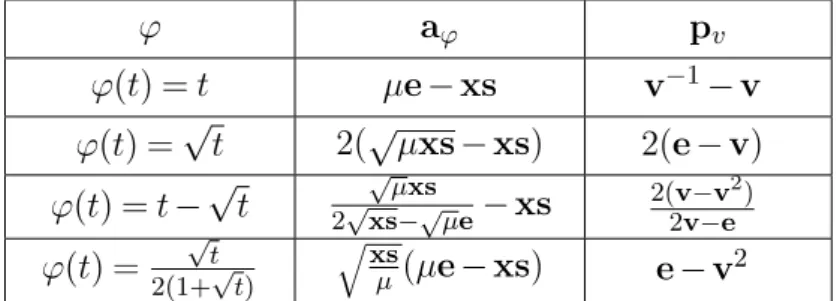
Table 1contains the classical AET functions used in the literature and the corresponding vectors a_ϕ and p_v.

ϕ a_ϕ p_v

ϕ(t) =t µe−xs v⁻¹−v

ϕ(t) =√

t 2(√

µxs−xs) 2(e−v) ϕ(t) =t−√

t

√µxs 2√

xs−√

µe−xs ^2(v−v2)

2v−e

ϕ(t) =

√t 2(1+√

t)

q_xs

µ(µe−xs) e−v² Table 1. AET functions used in the literature

Later on, Haddou et al. [24] proposed a family of smooth concave functions for mono- tone LCPs. However, it should be mentioned that they used other type of transformation of the central path system. They used functions ϕ:R+→R+ that satisfy the following conditions

H1. ϕ(0) = 0;

H2. ϕ∈ C³([0,+∞));

H3. ϕ⁰(t)>0, ∀t≥0;

H4. ϕ⁰⁰(t)≤0, ∀t≥0;

H5. ϕ⁰⁰⁰(t)≥0, ∀t≥0.

In the following subsection we introduce the new class of AET functions used in this paper.

2.3. New class of AET functions. We present the new class of AET functions which will be used in order to determine search directions.

Definition 2.4. Let ϕ: (ξ,∞)→R be a continuously differentiable, invertible function, such that ϕ⁰(t)>0, ∀t > ξ, where 0≤ξ <1. All functions ϕsatisfying the conditions AET1. ∃c₁∈R+, such that

ϕ(1)−ϕ(t²) 2t(1−t²)ϕ⁰(t²)

≤c₁, for all t > ξ.

AET2. ∃c₂∈R+, such that

4t²ϕ⁰(t²)^h(1−t²)ϕ⁰(t²)−ϕ(1) +ϕ(t²)ⁱ (ϕ(1)−ϕ(t²))²

≤c₂, for all t > ξ.

AET3. ∃c₃∈R⁺ such that the inequality

4t²(ϕ(1)−ϕ(t²))ϕ⁰(t²)−c₃ϕ(1)−ϕ(t²)² ≤ 4t²(1−t²)ϕ⁰(t²)²

≤ 4t²(ϕ(1)−ϕ(t²))ϕ⁰(t²) +ϕ(1)−ϕ(t²)² holds for all t > ξ,

belong to the new class of AET functions.

Let us introduce the following function: f : (ξ,∞)→R: f(t) = ϕ(1)−ϕ(t²)

t(ϕ⁰(t²)) , (2.10)

By using the function given in (2.10) we can give the definition of the new class of AET functions in the following way.

Proposition 2.1. The conditions given in Definition2.4 can be formulated in the follow- ing equivalent form:

AETa. ∃c₁∈R⁺, such that g(t) = _2(1−t^f(t)₂

) and |g(t)| ≤c₁, holds for all t > ξ;

AETb. ∃c₂∈R⁺, such that h(t) = ^{4(1−t2−tf(t))}

f(t)² = _(1−t^1−2tg(t)₂

)g(t)² and |h(t)| ≤c₂, holds for all t > ξ;

AETc. ∃c₃∈R+ such that the inequality tf(t)−c3

f(t)²

4 ≤1−t²≤tf(t) +f(t)² 4 holds for all t > ξ.

Proof. Using the function given in (2.10) after some calculations we obtain that conditions

AET1-3 can be formulated as the ones given in AETa-c.

Remark 2.1. The values of the parameters c₁,c₂ and c₃ will have influence on the well- definedness of the algorithm. For this, we will give a relation between these parameters.

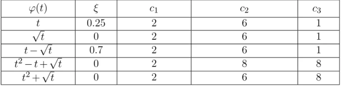
Table 2contains examples for ϕ belonging to this new family of functions, the value ofξ and the values c₁, c₂ and c₃. The values given in Table 2will be clear in the second part of the paper when we study the well-definedness of the algorithm. It should be mentioned that for the given values from Table2 the introduced algorithms are well defined and the complexity analyses work. However, there are several other acceptable values for these parameters.

ϕ(t) ξ c₁ c₂ c₃

t 0.25 2 6 1

√t 0 2 6 1

t−√

t 0.7 2 6 1

t²−t+√

t 0 2 8 8

t²+√

t 0 2 6 8

Table 2. Examples for ϕbelonging to the new class of AET function

Table 2 shows that most of the functions used in the literature from Table 1 belong to the new class of AET functions. However, it should be mentioned that the intervals

on which the functions ϕ are defined play important role in this approach. For example, ϕ(t) =t is only a member of this new class of AET functions if it is defined on a (ξ,∞) interval, where ξ is strictly positive. If ξ would be zero, then condition AET1 would not be satisfied for this function. Similar remark can be formulated in case of ϕ(t) =t−√

t.

Remark 2.2. The functions ϕ(t) =t²−t+√

t and ϕ(t) =t²+√

t are new in this AET technique. Up to our best knowledge they are the first AET functions in the literature, that have inflection point.

We can compare our new class of AET functions to the class of concave functions proposed by Haddou et al. [24].

Example 2.1. Consider the function ϕ(t) = log(1 +t), member of the class of concave functions introduced by Haddou et al. [24]. By using Definition 2.4, we can check that for this function condition AET3 is not satisfied.

In the following subsection we present the class of eligible kernel functions proposed in [9]

and the relationship between the kernel function approach and the AET technique.

2.4. Eligible kernel functions. The determination of search directions in case of IPAs can be realized by using kernel functions.

Definition 2.5. (Bai et al. [9]) A functionψ:R+→R⊕ is called kernel function if it is twice continuously differentiable and if the following conditions hold:

K1. ψ(1) =ψ⁰(1) = 0;

K2. ψ⁰⁰(t)>0, for all t >0;

K3. lim_t↓0ψ(t) = lim_t→∞ψ(t) =∞.

In some cases in the literature condition K3. of Definition 2.5 is used to define the notion of coercive kernel function, see [42, 43]. We can construct a barrier function Ψ :Rⁿ+→R in the following form:

Ψ(v) =

n X i=1

ψ(v_i), where v∈Rⁿ+.

Peng et al. [37] modified the second equation of the scaled system to d_x+d_s=−∇Ψ(v).

Using this and the scaled system (2.8), we have

d_x+d_s=−∇Ψ(v) =p_v=ϕ(e)−ϕ(v²)

vϕ0(v²) . (2.11) Hence, we can assign a corresponding kernel function to several functions ϕappeared in the AET technique in the following way, see [1, 36]:

ψ(t) =

Z t 1

ϕ(¯τ²)−ϕ(1)

¯

τ ϕ⁰(¯τ²) d¯τ , (2.12) where the function ψ should satisfy the properties K1.-K3. of Lemma 2.5.

Peng et al. [37] considered self-regular functions and in this way they reduced the theoretical complexity of long-step IPAs. The definition of self-regular functions is given below.

Definition 2.6. (Peng et al. [37]) A function ψ: (0,∞)→R, ψ∈ C² isself-regular if it satisfies the conditions

SR1. ψ(t) is strictly convex with respect to t >0 and ψ(t) = 0 at its global minimal point t= 1, i.e. ψ(1) =ψ⁰(1) = 0. Further, there exist positive constants ν₂≥ν₁>0 and p≥1, q≥1 such that

ν₁t^p−1+t^−1−q≤ψ⁰⁰(t)≤ν₂t^p−1+t^−1−q,∀t∈(0,∞); (2.13) SR2. For any t1, t2>0,

ψt^r₁t^1−r₂ ≤rψ(t₁) + (1−r)ψ(t₂), ∀r∈[0,1]. (2.14) The prototype self-regular kernel function is given by

Υp,q(t) = t^p+1−1

p(p+ 1)+t^1−q−1

q(q−1)+p−q

pq (t−1), (2.15)

where p≥1 and q≥1.

Bai et al [8] defined the class of eligible kernel functions.

Definition 2.7. (Bai et al. [8]) We call a kernel function eligible kernel function if it satisfies the following conditions:

EK1. tψ⁰⁰(t) +ψ⁰(t)>0, t <1;

EK2. ψ⁰⁰⁰(t)<0, t >0;

EK3. 2ψ⁰⁰(t)²−ψ⁰(t)ψ⁰⁰⁰(t)>0, t <1;

EK4. ψ⁰⁰(t)ψ⁰(βt)−βψ⁰(t)ψ⁰⁰(βt)>0, t >1, β >1.

Note that the class of eligible kernel functions contains some self-regular functions, as well as many non-self-regular functions as special cases, see [34]. However, it should be mentioned that all self-regular kernel functions Υp,q(t) with growth p≤1 belong to the class of eligible kernel functions.

Remark 2.3. Using (2.12) and (2.10) we have

ψ⁰(t) =−f(t). (2.16)

From this and Proposition 2.1 we obtain that if we have a kernel function, then using AETa-c we can check whether the corresponding function(s) ϕ do(es) belong to the new class of AET without calculating the functions ϕ. Furthermore, if we have a function ϕ, then by using the conditions given in Proposition2.1 we can check whether the conditions given in EK1-4 and K1-3 hold for the corresponding kernel function. Hence, we can compare functions from the class of new AET to corresponding kernel functions.

Example 2.2. Let ψ(t) =¹₂t−¹_t² be an eligible kernel function, see [34]. This is also a self-regular kernel function. Using (2.12) we have f(t) = −ψ⁰(t) = _t¹3 −t. Note that condition AETb from Proposition 2.1 or AET2 from Definition 2.4 is not satisfied in this case, which means that the function(s)ϕbelonging to this eligible and self-regular kernel function is (are) not members of the new class of AET. Note that we do not have to calculate ϕ to check this.

Remark 2.4. The functionϕ:R+→R+,ϕ(t) =tbelongs to the class of concave functions proposed by Haddou et al. [24]. Furthermore, the kernel function corresponding to this function is eligible kernel function. It should be mentioned that ϕ(t) =t belongs to the new class of AET functions if it is defined on (ξ,∞), where 0< ξ <1.

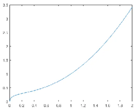
2.5. Special case of the new class of AET. Let us consider the special case mentioned in Subsection 2.3, ϕ: (0,∞)→R.

ϕ(t) =t²−t+√

t. (2.17)

Figure 1. Graph of the function given in (2.17).

The graph of the function given in (2.17) is shown in Figure2.17.

It is interesting that this function has inflection point. Up to our best knowledge this is the first AET function in the literature which has inflection point.

Using (2.4) and (2.9) we can calculate the corresponding a_ϕ and p_v in this case:

a_ϕ = µ

e−^x_µ^2s2²+^xs_µ −^qxs_µ

2^xs_µ −e+¹₂^q_xs^µ =2µ²√

xs−2x²s²√

xs+ 2µxs√

xs−2µxs√ µ 4xs√

xs−2µ√

xs+µ√

µ (2.18)

and

p_v=e−v⁴+v²−v

2v³−v+¹₂e = 2(e−v)(e+v²+v³)

4v³−2v+e . (2.19)

Hence, in our case

f(t) = 2(1−t⁴+t²−t)

4t³−2t+ 1 , (2.20)

and using (2.16), in our case when ϕis the function given in (2.17) we have f⁰(t) = −8t⁶+ 4t⁴+ 8t³−28t²+ 4t+ 2

(4t³−2t+ 1)² =−ψ⁰⁰(t). (2.21) f⁰⁰(t) = 4(8t⁶−36t⁵+ 108t⁴−20t³−6t²−12t+ 3)

(4t³−2t+ 1)³ =−ψ⁰⁰⁰(t). (2.22) Note that in case of kernel functions we haveψ⁰⁰(t)≥0. However, using (2.16) and (2.21) we can conclude that the kernel function corresponding to the function ϕgiven in (2.17) is not a kernel function in the sense, that ψ is not convex for all t >0. From the same reason we get that the kernel function belonging to the function ϕis neither self-regular, because in case of self-regular functions (2.13) should be satisfied. However, (2.21) takes positive and negative values as well. In case of eligible kernel functions ψ⁰⁰⁰(t)<0, hence we should have f⁰⁰(t)>0, fort >0. However, the expression given in (2.22) is not positive for allt >0. The kernel function corresponding to the functionϕgiven in (2.17) does not belong to the class of eligible kernel functions.

This function ϕ does not belong neither to the class of Haddou’s class of concave functions, because ϕ⁰⁰(t) = 2− ¹

4t√

t is not negative for all t≥0.

In the following subsection we present short-step IPAs for solvingP_∗(κ)-LCPs, that use this new class of functions in the AET technique to determine search directions.

2.6. New interior-point algorithms for solving P_∗(κ)-linear complementarity problems. Firstly, we deal with the determination of the search directions. For this, we

consider system (2.3), where a_ϕ depends on the function ϕused, which is member of the class new AET functions.

As special case, when ϕ(t) =t²−t+√

t,a_ϕ will be the expression given in (2.18).

We define the centrality measure δ:Rⁿ+×Rⁿ+×R+→R∪ {∞} as δ(x,s, µ) :=δ(v) = kp_vk

2 , (2.23)

where k · k denotes the standard Euclidean norm, and p_v is given in (2.9).

Consider the τ-neighbourhood of a fixed point of the central path as

N₂(τ, µ) :={(x,s)∈ F⁺:δ(x,s, µ)≤τ}, (2.24) where δ(x,s, µ) is given in (2.23), µ >0 is fixed and τ is a threshold parameter.

In Algorithm2.1 we define a whole class of IPAs for solvingP_∗(κ)-LCPs, which is based on the new class of AET functions.

Algorithm 2.1 : IPAs for P_∗(κ)-LCPs based on a new class of AET functions Let >0 be the accuracy parameter, 0< θ <1 the update parameter and τ the proximity parameter. Furthermore, a known upper bound κ of the handicap κ(Mˆ ) is given. Assume that for (x⁰,s⁰) the x^0Ts⁰=nµ⁰, µ⁰>0 holds such that δ(x⁰,s⁰, µ⁰)≤τ.

begin k:= 0;

while x^kTs^k > do begin

(determination of search directions)

compute(∆x^k,∆s^k)from (2.3) withϕbelonging to the new class of AET functions;

let x^k:=x^k+ ∆x^k and s^k :=s^k+ ∆s^k; (update of the parameter µ)

µ^k+1:= (1−θ)µ^k; k:=k+1;

end end

Remark 2.5. The default values of the parameters τ and θ will be given later in the complexity analysis of the algorithm.

Remark 2.6. If we consider the special case ϕ(t) =t²−t+√

t, then the default value of θ is _(200+100κ)^{1 √}_n and the default value ofτ is τ= _32+16κ¹ .

Remark 2.7. Note that using the function from (2.17) the proximity measure from (2.23) will be

δ(x,s, µ) = 1 2

e−v⁴+v²−v 2v³−v+¹₂e

. (2.25)

In the following section we present the complexity analysis of the IPAs using the new class of AET functions defined by conditions AET1-3 of Definition 2.4.

3. Complexity analysis

The first lemma shows the strict feasibility of the full-Newton step.

Lemma 3.1. Let (x,s)∈ F⁺ be given, such that δ(x,s;µ)≤ ^{√ 1}

1+4κ. For any function satisfying AET3 of Definition 2.4, we have that (x⁺, s⁺) ∈ F⁺.

Proof. It should be mentioned that only the right hand side of AET3 should be satisfied in this lemma, namely:

4t²(ϕ(1)−ϕ(t²))ϕ⁰(t²) +ϕ(1)−ϕ(t²)²≥4t²(1−t²)ϕ⁰(t²)², t > ξ. (3.1) We have

x(α)s(α) = (x+α∆x)(s+α∆s) =xs+α(s∆x+x∆s) +α²∆x∆s

= µv²+µvα(d_x+d_s) +α²µd_xd_s (3.2)

= µ((1−α)v²+α(v²+vp_v+αd_xd_s).

Our aim is to show that µα(v²+vp_v+αd_xd_s)≥0. We have p_v=d_x+d_s and using the notations q_v:=d_x−d_s it can be seen that

d_xd_s= p²_v−q²_v

4 . (3.3)

Using the definition of p_v given in (2.9) we obtain that (3.1) is equivalent with vp_v+p²_v

4 ≥e−v², (3.4)

which leads to

v²+vp_v≥e−p²_v

4 . (3.5)

Using (3.2), (3.3) and (3.5) we have x(α)s(α)

µ = (1−α)v²+α v²+vp_v+αp²_v

4 −αq²_v 4

!

≥(1−α)v²+α e−(1−α)p²_v

4 −αq²_v 4

!

.

We have x(α)s(α)

µ ≥0, if

(1−α)p²_v

4 −αq²_v 4

_∞

≤1 holds.

From [16] we obtain

kq_vk ≤√

1 + 4κkp_vk= 2√

1 + 4κδ. (3.6)

Then, we have

(1−α)p²_v

4 −αq²_v 4

_∞

≤(1−α)kp_vk²

4 +αkq_vk² 4

≤(1−α)kp_vk²

4 +α(1 + 4κ)kp_vk² 4

= (1 + 4ακ)δ²≤(1 + 4κ)δ².

This means that

(1−α)p²_v

4 −αq²_v 4

_∞

≤1 holds if we have δ≤ 1

√1 + 4κ. In this way the lemma is proven.

In the following lemma we analyse the conditions under which the Newton process is quadratically convergent.

Lemma 3.2. Suppose that δ(x,s;µ)≤ ^{√ 1}

1+4κ. Let (x,s)∈ F⁺ and v¯=

sx⁺s⁺

µ be given.

For any function ϕsatisfying AET1 and AET2 of Definition 2.4, we can say that after a primal-dual Newton barrier step we have:

δ(x⁺,s⁺;µ)≤c₁(c₂+ 2 + 4κ)δ(x,s;µ)², where c₁, c₂∈R+.

Proof. It should be noted that in the proof we will use the form AETa and AETb of Proposition 2.1. Using Proposition 2.1 and (2.23) we get

δ(x⁺,s⁺;µ) := kp¯vk

2 =(e−v¯²)g(¯v), (3.7) where the function g is given in Proposition (2.1). Using the assumption that ∃c₁∈R+, for which |g(t)| ≤c₁, we obtain

δ(x⁺,s⁺;µ)≤c₁e−¯v². (3.8) We know from (3.2) that

e−v¯²=

e−x⁺s⁺ µ

=

e−v²−vp_v−p²_v 4 +q²_v

4

. (3.9)

Using condition AETb of Proposition 2.1 we have e−v²−vp_v = h(v)p²_v

4 . (3.10)

Using (3.6), (3.9) and (3.10) we obtain

e−v¯² ≤ e−v²−vp_v+

p²_v 4

+

q²_v 4

≤(2 +c₂+ 4κ)δ². (3.11) From (3.8) and (3.11) we have

δ(x⁺,s⁺;µ)≤c₁(c₂+ 2 + 4κ)δ(x,s;µ)², which proves the lemma.

In the next lemma we investigate the effect of the full-Newton step on the duality gap.

Lemma 3.3. Letδ:=δ(x,s;µ)and suppose that the vectorsx⁺ ands⁺are obtained using a full-Newton step, thus x⁺=x+ ∆x and s⁺ =s+ ∆s. For any function ϕ satisfying AET3 of Definition 2.4 with c₃∈R+, we have that

x^+Ts⁺≤µ(n+ (c₃+ 1)δ²).

Proof. Note that only the left hand side of AET3 will be used in this proof, namely 4t²(ϕ(1)−ϕ(t²))ϕ⁰(t²)−c₃ϕ(1)−ϕ(t²)²≤4t²(1−t²)ϕ⁰(t²)², t > ξ. (3.12) Using the definition of p_v in (2.9) we get that (3.12) is equivalent with

vp_v−c₃p²_v

4 ≤e−v². (3.13)

From (3.2) and (3.13) we get 1

µx⁺s⁺=v²+vp_v+d_xd_x≤e+c₃

4p²_v+d_xd_s. After some calculations we have

x^+Ts⁺=e^T(x⁺s⁺)≤µ(e^Te+c₃

4e^Tp²_v+e^Td_xd_s)

=µ(n+c₃

4 kp_vk²+d^T_xd_s)

≤µ(n+c₃δ²+δ²) =µ(n+ (c₃+ 1)δ²).

The last inequality holds, since

d^T_xd_s =kd_x+d_sk²− kd_x−d_sk²

4 ≤ kd_x+d_sk²

4 =kp_vk² 4 .

The next lemma examines the effect which a Newton step followed by an update of the parameter µ has on the proximity measure.

Lemma 3.4. Suppose that δ(x,s;µ)≤^{√ 1}

1+4κ. Let v⁺=

r x⁺s⁺

µ⁺ , whereµ⁺= (1−θ)µ and let η =√

1−θ. For any function ϕ satisfying AET1 and AET2 of Definition 2.4 with c₁, c₂∈R+, after a primal-dual Newton step we have:

δ(x⁺,s⁺;µ⁺)≤ c₁ η²

θ√

n+ ((c₂+ 2) + 4κ)δ².

Proof. In the proof we will use the form AETa and AETb of Proposition 2.1. Using the definition of the proximity measure given in (2.9) we have

δ(x⁺,s⁺;µ⁺) =(e−(v⁺)²)g(v⁺). From condition AETa of Proposition 2.1 , we get

δ(x⁺,s⁺;µ⁺)≤c₁e−(v⁺)². (3.14) Furthermore,

e−(v⁺)² =

e− 1 η²

x⁺s⁺ µ

=

e− 1

η² v²+vp_v+p²_v 4 −q²_v

4

!

= 1

η²

η²e− v²+vp_v+p²_v 4 −q²_v

4

!

= 1

η²

−θe+e−v²−vp_v−p²_v 4 +q²_v

4

. (3.15)

From (3.10), (3.14), (3.15) and condition AETb of Proposition2.1 we obtain δ(x⁺,s⁺;µ⁺) ≤ c₁

η² kθek+e−v²−vp_v+

p²_v 4

+

q²_v 4

!

≤ c₁ η²

θ√

n+ ((c₂+ 2) + 4κ)δ². (3.16) In the following lemma we set the values of the parameters θ and τ and we prove that for these values the IPAs using the new class of AET functions are well defined.

Lemma 3.5. Let ϕ: (ξ,∞)→R satisfying AET1-3 of Definition 2.4. Consider n≥1,

θ= ²

25c2(2+κ)√

n and τ =_2c ¹

2(2+κ). If c1< ^100c_41c ²⁻⁴

2+50 and c2>¹₂, then we have δ(x⁺,s⁺;µ⁺)< τ,

hence the IPAs defined in Algorithm 2.1 are well defined.

Proof. We suppose that τ = _2c ¹

2(2+κ) and c₂> ¹₂. From here we have _2c ¹

2(2+κ) < _2+κ¹ <

√ 1

1+4κ. Using this and the assumption that AET1-3 of Definition 2.4 are satisfied, from Lemma 3.1 we get that (x⁺,s⁺)∈ F⁺.

Using Lemma 3.4 we have

δ(x⁺,s⁺;µ⁺) ≤ c₁ η²

θ√

n+ ((2 +c₂) + 4κ)δ². (3.17) Considering θ= ²

25c2(2+κ)√

n we get θ√

n= 2

25c₂(2 +κ). (3.18)

Moreover, using n≥1,κ≥0 we have 1

1−θ ≤ 1 1−_50c²

2

= 25c2

25c₂−1. (3.19)

Substituting the value of τ in (3.17) and using κ≥0, (3.18) and (3.19), we get δ(x⁺,s⁺;µ⁺) ≤ c₁· 25c₂

25c₂−1

2

25c₂(2 +κ)+ (c₂−6 + 8 + 4κ) 1 (2c₂(2 +κ))²

!

= c₁· 25c₂ 25c₂−1

4

25(2c₂(2 +κ))+ c₂−6

4c²₂(2 +κ)²+ 4(2 +κ) 4c²₂(2 +κ)²

!

=

≤ c₁· 25c₂ 25c₂−1

1 2c₂(2 +κ)

4

25+c₂−6 4c₂ + 2

c₂

= c₁ 25c₂ 25c₂−1

41c₂+ 50 100c₂

1

2c₂(2 +κ)= c₁(41c₂+ 50)

100c₂−4 τ. (3.20) The obtained result should be less than τ, hence usingc2>¹₂ >₂₅¹, we get

c₁< 100c₂−4

41c₂+ 50, (3.21)

which gives the result.

Remark 3.1. It should be mentioned that the parameters c₁ and c₂ of the functions given in Table 2 satisfy the condition c₂>¹₂ and c₁< ^100c_41c ²⁻⁴

2+50.

The following lemma gives upper bound on the number of iterations.

Lemma 3.6. Consider ϕ: (ξ,∞)→R satisfying AET1-3 of Definition 2.4. Let n≥1, θ=_25c ²

2(2+κ)√

n, τ =_2c ¹

2(2+κ), c₁<^100c_41c ²⁻⁴

2+50 and c₂>¹₂ and c₃<16c²₂−1. We assume that the pair (x⁰,s⁰)is strictly feasible, µ⁰=^(x

0)^Ts⁰

n and δ(x⁰,s⁰;µ⁰)< τ. Let x^k ands^k be the two vectors obtained by the algorithms given in Algorithm 2.1 after k iterations. Then, for

k≥

&

1

θlogµ⁰(n+ 1) ε

'

we have (x^k)^Ts^k< ε.

Proof. From Lemma 3.3 and c₃<16c²₂−1 we have

x^kTs^k ≤ µ^k n+ (c₃+ 1)· 1 (2c₂(2 +κ))²

!

= (1−θ)^kµ⁰ n+ (c₃+ 1)· 1 (2c₂(2 +κ))²

!

<(1−θ)^kµ⁰(n+ 1). (3.22) The condition (x^k)^Ts^k< ε holds if

(1−θ)^kµ⁰(n+ 1)< ε. (3.23)

Taking the logarithm of both sides of (3.23) we have

klog (1−θ) + logµ⁰(n+ 1)<logε.

Using that −log (1−θ)≥θ finally we get

kθ≥logµ⁰(n+ 1)−logε= logµ⁰(n+ 1)

ε ,

which proves the lemma.

Remark 3.2. Condition c₃<16c²₂−1 is satisfied for all functions given in Table 2.

Theorem 3.1. Let ϕ: (ξ,∞)→R satisfying AET1-3 of Definition 2.4. Consider n≥1,

θ= ²

25c2(2+κ)√

n andτ =_2c ¹

2(2+κ). If c₁<^100c_41c ²⁻⁴

2+50, c₂> ¹₂ and c₃<16c²₂−1, then the IPAs given in Algorithm 2.1 require no more than

O (2 +κ)√

nlog(n+ 1)µ⁰

!

interior-point iterations.

In the following subsection we analyse the special case when ϕ(t) =t²−t+√

t, which is the first AET function which has inflection point.

3.1. Special case. The first step of this research was to define and analyse an IPA using a new type of function in the AET technique, which has inflection point. From this analysis we built up the new class of AET functions. Hence, in this subsection, we summarize the corollaries of the lemmas presented in the previous part in the special case when ϕ(t) =t²−t+√

t.

Corollary 3.1. Let (x,s)∈ F⁺ be given, such that δ(x,s;µ)< ^{√ 1}

1+4κ. In case of ϕ(t) = t²−t+√

t we have that (x⁺,s⁺)∈ F⁺.