Non-technical loss detection at unregistered points in power distribution systems
Márton Greber, Attila Fodor, Attila Magyar
University of Pannonia, Department of Information Technology, Egyetem u. 10, 8200 Veszprém. Hungary, e-mails: greber.marton@virt.uni-pannon.hu,
fodor.attila@virt.uni-pannon.hu, magyar.attila@virt.uni-pannon.hu
Abstract: In this paper a non-technical loss (NTL) diagnostic method is proposed which considers faults at unregistered points in the distribution network. The method relies on the concept of smart grid, where every consumer is equipped with smart meters. Existing line segments are split up in order to detect and isolate faults at arbitrary points between metered points. The goal is to adjust the power and distance of these nodes such that the measured voltage profile is obtained. This results in a non-linear optimization problem, which is approximated using a genetic algorithm. Based on conservation of energy a local evaluation method is worked out. This is used to reduce the enormous search space of a fully extended network. The computational burden is further relaxed by showing the applicability of parallel computation for both diagnostic techniques.
Keywords: non-technical faults; fault detection; smart grid; distribution system; genetic algorithm;
1 Introduction
The low-voltage grid is responsible for distributing power to end consumers.
Because of this, the number of residential connections and human interaction is far greater than in the higher voltage level subsystems. Activities regarding the theft of electricity can be observed. The notion of non-technical loss (NTL) is a collective concept, it can originate from: meter tampering, measurement and billing errors or illegal connection. In any case it leads to consumed power which goes unaccounted, thereby contributing to financial deficit. [1] By tampering a metering device or conducting illegal connections on the utility equipment technical risks and reliability issues arise.
Tampering measurement devices, and fooling the meter readings is a relatively long known problem, to which working solutions are to be found. Through advanced features like detecting magnetic fields or the utilization of a so called “Hardware Against Software Privacy” key the trust and confidence at registered points gets
well established. [2] On the other side, dedicated diagnostic hardware can be also placed throughout the network. These are invasive methods meaning they require additional components, and active methods can be performed in the form of signal injection. By observing the distribution system state, if high NTL is estimated, the good customers can be disconnected and through a distortion signal the illegal point’s performance can be reduced. [3] However, this imposes several security concerns if a good customer stays on during the purging period. A gentler approach is the injection of high frequency components, which are captured at installed LC trap points. These signals are affected by NTL thereby allow for detection, and isolation of edges. [4] Moreover if the installation of LC traps is infeasible a comparison between a no-load and on-load high frequency impedance calculation can serve as an indicator for the presence of NTL. [5]
The notion of smart grid combines the concepts of power and information system by forming a complex cyber-physical system. Among others, residential consumers are equipped with smart meters, enabling the reporting of measurements in 15- minute periods. Information from a neighbourhood is collected by a data concentrator, which sends the packets to the utility server. [6] This increased amount of information offers new possibilities in the diagnosis of NTLs. [7] There are two main approaches for detection: data oriented and network model oriented.
This paper focuses on a model-based approach, which requires no cumulative dataset and learning process. On the other hand, the technical modelling requires domain specific knowledge and the resulting model tends to be complex. [8] In order to combat the complex nature of the diagnosis one can apply switching logic to various parts of the network. In this case, the task is to set the states of the switches in such a manner that a close to nominal operating condition is acquired, parts affected by NTL become isolated. [9] Utilizing first engineering principles the network can be broken down into elementary topologies where the condition for nominal operation is easier to compute. [10] In general, the indicator of NTL is the difference between an expected nominal voltage profile and the measured one. The goal is to reproduce the measured one through optimization. [11] These problems are often solved through soft computing techniques, which are computationally heavy. Efficient methods can be developed utilizing for example the topological properties of radial networks. Heuristics based on the direction of power flow allow for better compensation procedures for a network having power deficit by NTL.
[12]
The parameters of fault are considered the missing power and the distance from neighbouring measured loads. All off the above-mentioned methods inspect the diagnosis of registered points – like cross verification – moreover methods which mention localisation give only estimation whether a given line segment is faulty or not. [13] By taking a given edge, splitting it up and inserting a hypothetical fault consumer, NTL at unknown location can be diagnosed. [14] The approach is based on the conservation of energy, and results in an optimization problem concerning network structure and load as well. [15] A similar idea can be found in high voltage
direct current transmission systems for diagnosing fault parameters of a long line segment. [16] In this case, the solution was achieved through a genetic algorithm approach. Moreover, the optimal placement of compensator capacitor banks poses a similar optimization problem, however quite often the location search space consists only from existing nodes. [17] From the above-mentioned reviews, it is clear that there is a need for further research in diagnosing and estimating fault parameters between metered nodes at arbitrary locations. The aim of this paper is to present a formal description to this problem which can be used to develop a general fault diagnostic expression. The approximate solution is presented as a genetic algorithm. The search space is taken into account by presenting search space reduction technique.
2 Distribution system modelling
The main components of the distribution system are the medium voltage to low voltage transformer station, also called feeder point, the distribution line and the consumer points. Throughout this work, single phase representation is used. The feeder point is represented as a voltage generator, Norton equivalent. The line segments are RL branches, the effect of mutual coupling is neglected. The type of the residential loads is constant P, Q. Every one of them is equipped with smart meter, capable of measuring active(P) and reactive(Q) power, voltage and current root mean square (RMS) values. Furthermore, it is assumed that NTLs can be found between metered points at arbitrary location, however one edge can contain one fault at most.
The topology of the network is described by the incidence matrix: 𝑨 ∈ {−1,0,1}𝑛×𝑚, where 𝑛 is the number of vertices and 𝑚 is the number of edges in the graph of the system. The entries of the incidence matrix are described in equation (1). Vectors are defined for the electrical quantities, an element of these corresponds to an edge in the graph: 𝒀-admittance, 𝑰-current, 𝑼-voltage and 𝑺- power. All of these quantities are complex numbers: 𝒀, 𝑰, 𝑼, 𝑺 ∈ ℂ𝑚×1 . However, calculations are performed referred to the edges of the graph, in the bus reference frame. A singular transformation utilizing the incidence matrix yields the bus admittance matrix: 𝒀𝑏𝑢𝑠= 𝑨𝑑𝑖𝑎𝑔(𝒀)𝑨𝑇. All the other quantities can be transformed into the bus reference frame by using the vertex-edge property of the incidence matrix, for example: 𝑼𝑏𝑢𝑠= 𝑨𝑼.
𝑎𝑖,𝑗= {
0 edge j is not connected to vertex i 1 edge j is pointing towards vertex i
−1 edge j is pointing away from vertex j
(1) Then, Ohm’s law can be formulated the following way: 𝑼𝑏𝑢𝑠= 𝒀𝑏𝑢𝑠−1𝑰𝑏𝑢𝑠. The electrical parameters of the distribution system components are collected in separate vectors. 𝒀𝑔𝑒𝑛, 𝑰𝑔𝑒𝑛 describe the feeder point’s Norton equivalent parameters. 𝒀𝑙𝑖𝑛𝑒
contains the distribution line admittances. Finally, 𝑰𝑙𝑜𝑎𝑑, 𝑺𝑙𝑜𝑎𝑑 contain the calculated current and the specified complex power at the residential consumer edges. The power flow equations are given as a set of non-linear equations in matrix form, see equation (2). The first equation is Ohm’s law in the bus reference frame, where component-describing vectors are explicitly stated. The second equation is responsible for the constant P, Q load modelling.
{𝑼𝑏𝑢𝑠= 𝑨𝑑𝑖𝑎𝑔(𝒀𝑔𝑒𝑛+ 𝒀𝑙𝑖𝑛𝑒)𝑨𝑇𝑨(𝑰𝑔𝑒𝑛+ 𝑰𝑙𝑜𝑎𝑑)
𝑺𝑙𝑜𝑎𝑑 = 𝑑𝑖𝑎𝑔(𝑼𝑏𝑢𝑠)𝑨𝑰𝑙𝑜𝑎𝑑∗ (2)
The known parameters are the incidence matrix, the admittances, the Norton equivalent generator currents and the load power values. The task is to find the bus voltages such that the specified power values are held.
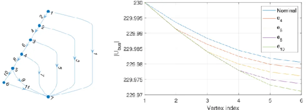
Figure 1 Left: graph of the network, edge notations: generator: 1, loads: 3, 5, 7, 9, 11, line segments:
2, 4, 6, 8, 10. Right: NTL on various points of the network and the change in voltage drop
2.1 Non-technical loss indicators
NTLs produce an undesirable effect in the power network: more power needs to fed into it than it is expected. Therefore, the analysis of NTLs is heavily reliant on the conservation of energy. Measured quantities from this point on are denoted by tilde.
If the sum of measured feeder current is greater than the sum of all measured customers there is a fault in the network. This follows from Kirchhoff’s current law (KCL): ∑𝑰̃𝑔𝑒𝑛 > ∑𝑰̃𝑙𝑜𝑎𝑑. Let us now consider the consumed powers. By taking the power measurements and calculating the power flow, the losses can be estimated.
If the measured generated power is greater than the measured load plus the calculated losses, there is a fault condition: ∑𝑺̃𝑔𝑒𝑛> ∑𝑺̃𝑙𝑜𝑎𝑑+ ∑𝑺𝑙𝑜𝑠𝑠. Furthermore, if more current is flowing through the distribution lines than expected, the increased current produces a greater voltage drop on it. Therefore, if the difference between the measured bus voltages and the calculated voltages is greater than zero, there is NTL in the network: 0 < ∑𝑛𝑖=1(𝑢̃𝑏𝑢𝑠𝑖− |𝑢𝑏𝑢𝑠𝑖|)2. Since the measured voltage is an RMS value, the bus voltages from the complex power flow must be taken as the absolute value. All of these expressions can be used for fault
detection (FD). A simple example is shown in Figure 1. Edge 1 is the feeder, edges 3, 5, 7, 9, 11 are the load edges, the others are line edges. The nominal voltage profile is shown in blue, then separate faults are inserted onto the line edges. The difference between nominal and faulty profile is clear to see on Figure 1.
3 Network extension-based diagnosis
In the previous example the NTL was somewhere on the line, there was no information about it in the graph. In order to formulate a diagnostic method for such fault, the network needs to be extended. The main idea is, that all the distribution line segments are split up according to a division point and a hypothetical fault consumer is inserted (see Figure 2).
Figure 2 Left: the network before the extension, edges 2 and 4 are the lines to be split. Right: the extended network, edges 6 and 8 are the hypothetical fault load edges
Dividing the existing line segment impedance through the division point (0 < 𝑑 <
1) allows to set the fault distance from the neighboring edges. The inserted hypothetical fault consumer is modelled like all the other real customers. Setting the consumed power value allows for adjusting the fault magnitude. In order to create a fully extended network all the line segments need to be located. For every edge insert a new vertex, route the old-line segment to this vertex and add a new edge pointing from the fault node to the original edge’s end node. For example on Figure 2: old edge 2, new fault node 4, route edges 1 → 4, insert new edge 7 route 4 → 2. Then a so-called extended network is obtained, which is described by quantities denoted by a hat: 𝑨̂, 𝑰̂, 𝑼̂, 𝒀̂, 𝑺̂. The number of vertices is 𝑛̂, the number of edges is 𝑚̂ in the extended network. The hypothetical fault powers of the inserted edges are collected in 𝑺𝑓𝑎𝑢𝑙𝑡, the distance describing division points are collected in 𝑫𝑓𝑎𝑢𝑙𝑡. These quantities need to be incorporated in the power flow calculation, resulting in the extended network power flow equations (equation (3)). The hypothetical fault power values need to be substituted into the load power vector, therefore 𝑺̂𝑙𝑜𝑎𝑑 becomes a function of the fault power. Moreover, the extended line
admittance vector becomes a function of the division point vector, since the extended network’s line admittances are determined according to them.
{𝑼̂𝑏𝑢𝑠= 𝑨̂𝑑𝑖𝑎𝑔(𝒀𝑔𝑒𝑛+ 𝒀̂𝑙𝑖𝑛𝑒(𝑫𝑓𝑎𝑢𝑙𝑡))𝑨̂𝑻𝑨̂(𝑰𝑔𝑒𝑛+ 𝑰̂𝑙𝑜𝑎𝑑)
𝑺̂𝑙𝑜𝑎𝑑(𝑺𝑓𝑎𝑢𝑙𝑡) = 𝑑𝑖𝑎𝑔(𝑼̂𝑏𝑢𝑠)𝑨̂𝑰̂𝑙𝑜𝑎𝑑∗ (3) The NTL diagnosis is described as a non-linear optimization problem in equation (4). Given a set of fault parameters, the non-linear load flow equations are solved.
Measurement data is only available for the vertices in the original network (vertex indexes: 1 … 𝑛). Therefore, the difference between measured and calculated voltages are calculated. The goal of the fault diagnostic method is to use the extended network, and adjust the fault parameters (𝑺𝑓𝑎𝑢𝑙𝑡, 𝑫𝑓𝑎𝑢𝑙𝑡), such that the original voltage profile is obtained.
min𝑫𝑓𝑎𝑢𝑙𝑡,𝑺𝑓𝑎𝑢𝑙𝑡 ∑(𝑢̃𝑏𝑢𝑠𝑖− |𝑢̂𝑏𝑢𝑠𝑖(𝑫𝑓𝑎𝑢𝑙𝑡, 𝑺𝑓𝑎𝑢𝑙𝑡)|)2
𝑛
𝑖=1
𝑠. 𝑡. : ∑ 𝑠𝑓𝑎𝑢𝑙𝑡𝑖
𝑚̂ −𝑚
𝑖=1
= 𝑠𝑚𝑖𝑠𝑠𝑖𝑛𝑔
∀𝑖 ∈ {1 … 𝑚̂ − 𝑚}, 0 < 𝑑𝑓𝑎𝑢𝑙𝑡𝑖< 1
(4)
The formulation is bounded by constraints to manage feasibility. The sum of the injected hypothetical fault nodes must equal the recorded missing power.
Additionally, all the division points must be between 0 and 1.
A solution to the constrained non-linear optimization problem is achieved through an evolutionary algorithm. A chromosome is a possible solution to the problem. In this case two simultaneous arrays of the fault parameters. Many random chromosomes are generated to form a generation. Chromosomes in a generation are ranked by their fitness value. It is a measure of how good of a solution they are, evaluated according to the objective function. The optimization constraints are enforced through a penalty function. This assigns a percentage increase in the fitness function if the constraints are violated. The top 𝑥% go immediately into the upcoming generation, this is called elitism. New chromosomes are formed by taking existing ones and recombining them. Finally, some chromosomes are perturbed randomly in some of their values, which is called mutation. Through these three simple steps a new generation is formed. The process continues until the number of maximum generations is reached or a solution is found.
4 Search space reduction technique
By accomplishing a total network extension, the search space becomes enormous.
In order to reduce it, a local evaluation-based technique is proposed. The idea came
from discrete convolution where one takes a kernel and it is shifted through the network. Through this process new information is gathered. This is translated into power system analysis. The local evaluation structure, the so-called kernel is depicted in Figure 3. There are four measured load points 𝑣1… 𝑣4 and the conservation of energy is observed in the middle line segment, depicted in red.
Figure 3 Local evaluation structure, vertices 𝑣1… 𝑣4 are metered points. Line segment 𝑍2 is split up, and then a hypothetical fault is inserted at vertex 𝑣𝑓
There are three unknowns: 𝑍𝑓 - the fault distance representing impedance, 𝐼𝑓 - the fault current and 𝑈𝑣𝑓 - the bus voltage at the point of NTL. Applying Kirchhoff’s current law, three equation can be formulated for vertices 𝑣2, 𝑣𝑓, 𝑣3. These are a set of linear equations. One can solve for 𝐼𝑓 to obtain a verification indicator.
{
𝑈𝑣1− 𝑈𝑣2
𝑍1 +𝑈𝑣𝑓− 𝑈𝑣2
𝑍𝑓 − 𝐼1= 0 : vertex 𝑣2
𝑈𝑣2− 𝑈𝑣𝑓
𝑍𝑓 +𝑈𝑣3− 𝑈𝑣𝑓
𝑍2− 𝑍𝑓 − 𝐼𝑓= 0 vertex 𝑣𝑓 𝑈𝑣4− 𝑈𝑣3
𝑍3 +𝑈𝑣𝑓− 𝑈𝑣3
𝑍2− 𝑍𝑓 − 𝐼2= 0 vertex 𝑣3
(5)
The question arises that what happens if a fault is present not in the middle, rather on one of the side line segments of the structure? A so-called kernel shift procedure is developed to overcome this process. Let us consider a “street” of 8 customers in a series topology, where a fault is present between vertices 4, 5. The kernel evaluation results are depicted in Table 1.
Table 1 Kernel shift evaluation Bus in kernel
1 2 3 4 5 6 7 8
Starting bus 1 ✓ ✓ ✓ ✓
2
3
4
5 ✓ ✓ ✓ ✓
The columns denote the distribution line buses, whereas the rows denote the starting position of the kernel. If the evaluation results in 𝐼𝑓 = 0, a ‘✓’ (verified) is drawn, else ‘’ (not verified) is present. The edge between vertices 4,5 is faulty, all the positions with starting bus = 1 and 5 are locally fault free, the conservation of energy is valid. All the other kernel positions contain the faulty edge. According to KCL there must be a current deficit therefore these edges are marked as not verified.
The set of fault edges can be determined by performing a set minus operation on the verified and not verified sets. These sets contain edges of the network described as a pair of vertices.
Verified = {{1,2}, {2,3}, {3,4}, {4,5}, {5,6}, {6,7}, {7,8}}
Not verified = {{2,3}, {3,4}, {4,5}, {5,6}, {6,7}}
Faulty = Not verified\Verified = {{4,5}}
(6) Diagnosing the network in such local units of 4 vertices, allows for a fast checking process to observe which edges are fault free, thereby reducing search space.
However, the method has some limitations. Unique isolation of the fault is only possible if and only if, at least three verified edges are present before and after the fault location (see Figure 4).
Figure 4 Uniquely determined faults: the faulty edges are separated by at least three verified edges, thereby unique isolation is possible
Figure 5 Three-edge criteria bottleneck: the faulty edges are separated by only two edges, in between edges are marked as faulty.
If the above-mentioned criteria is not fulfilled (see Figure 5) no matter what the fault status of the inner edges is, they become all marked as faulty. This is a case where the search space reduction technique has a bottleneck. It introduces edges, which may or may not be truly faulty; this is the case where the general optimization method needs to be applied.
5 Complete fault diagnostic process
The above-mentioned two methods can be used together in order to form a complex diagnostic procedure. The voltage criteria need to be checked, if the measured and calculated voltage profiles are different, there is a fault else, there is no fault, the process exits. In case of fault, one takes the local evaluation kernel and it is shifted through the network. Edges denoted as ‘Faulty’ are marked. These marked edges are used to construct a partially extended network. Finally, the genetic algorithm is started to approximate the fault parameter, but in this case with a much smaller search space.
Taking into consideration the reduction technique, soft computing methods like the genetic algorithm are computationally heavy and provide only approximate solutions. By considering that the fitness evaluation within a generation is computationally independent, and so are the kernel evaluations at different positions, such parts of the method can be executed in a parallel manner. This also offers the utilization of distributed resources and so horizontal scaling.
Figure 6 Case study network topology: blue vertices and edges denote the nominal network, the red components denote the partially extended network, which form the search space.
Figure 7 Voltage profile of the network: the blue plot denotes the nominal voltage profile, whereas the red line indicates the measured voltages. There is a difference between them. It indicates the presence of NTL in the network.
5.1 Case study
In order to demonstrate the procedure in action, a simulation case study was created.
It is based on the curated IEEE low-voltage test feeder. We chose to make our own, in order to test the capabilities on a larger network. It contains 4 streets with 15 loads each. The distance between customers is 45 − 50m. Average RL parameters
where taken from the different cable types. For the simulation, parallel implementation of the proposed method was run on 3 PCs by utilizing MATLAB’s distributed computing server. The networks topology is shown in Figure 6. 5 faults were inserted into the network (shown in red). Through simulation, measurement data was generated to represent real working conditions. The expected network operation was calculated by using only the components marked with blue. The voltage profile of the network is shown in Figure7. The nominal or also called expected profile is shown with blue. With red - which is shadowed by green - the measured profile. Finally, green represents the voltage profile which was the result of the diagnostic procedure. At first sight the match is quite good.
Table 2 Case study genetic algorithm based optimization results
Vertex Id 𝒔𝒇𝒂𝒖𝒍𝒕 𝒔̂𝒇𝒂𝒖𝒍𝒕 𝒅𝒇𝒂𝒖𝒍𝒕 𝒅̂𝒇𝒂𝒖𝒍𝒕
66 120 − 20𝑖 167.90 − 28.95𝑖 0.5 0.15
64 50 − 10𝑖 310.90 − 53.60𝑖 0.6 0.45
69 − 71.12 − 12.26 − 0.70
65 300 − 70𝑖 19.04 − 3.28𝑖 0.8 0.68
350 − 80𝑖 410.06 − 69.14
62 250 − 50𝑖 289.37 − 49.89𝑖 0.2 0.01
67 − 0 + 0𝑖 − −
68 − 0 + 0𝑖 0.4 −
63 100 + 0𝑖 0 + 0𝑖 0.4 −
350 − 50𝑖 289.37 − 49.89𝑖
The graph presented above is the result of the network extension method. In Table 2 the detailed results regarding the best chromosome of the genetic algorithm are shown. The fault at node 66 was a fault alone, the kernel could isolate it, and the genetic algorithm's results are shown in the first section of the table. 𝑠𝑓𝑎𝑢𝑙𝑡 and 𝑑𝑓𝑎𝑢𝑙𝑡 represent the real values, 𝑠̂𝑓𝑎𝑢𝑙𝑡 and 𝑑̂𝑓𝑎𝑢𝑙𝑡 represent the approximated final values. The fault power is quite a good match. The fault distance has an error of 0.35. Next let’s observe the section of nodes 20 − 23. As it can be seen in the table it was a section where there was a non-faulty edge between faults. This is why we have here 3 hypothetical insertions, the kernel's 3 edge rule. Here the individual fault powers are totally mixed, however total fault power, is well approximated. The same is the case for the last branch where an even bigger uncertainty was set by having two valid edges separate the fault. Overall, it can be seen that the detection is appropriate. On the contrary, the fault isolation works only good for unique faults, in that case fault parameters can be determined. In any case where the kernel limitations are violated the fault is isolated as a hotspot region. And fault parameters especially fault power is an approximation for the whole hot-spot.
Conclusion
A model-based fault detection method has been presented in this work for the handling of NTLs in distribution networks. The problem is traced back to a non- linear optimization problem. A solution was found by utilizing genetic algorithms.
Computational burden was considered by introducing a search space reduction technique and parallel computing approach. Some interesting ideas for future applications are the implementation of the local kernel evaluation method on the data concentrator level for decentralized detection. The genetic algorithm could be improved through heuristics based on topology properties. Furthermore, the proposed method could be applied for faults in other physical domains with similar characteristics for example leakages in pipe networks.
Acknowledgement
Project no. 131501 has been implemented with the support provided from the National Research, Development and Innovation Fund of Hungary, financed under the K_19 funding scheme. A. Magyar was supported by the Janos Bolyai Research Scholarship of the Hungarian Academy of Sciences. Attila Magyar was supported by the UNKP-20-5 new national excellence program of the Ministry for Innovation and Technology.
References
[1] F. B. Lewis, "Costly ‘Throw-Ups’: Electricity Theft and Power Disruptions,"
The Electricity Journal, vol. 28, pp. 118-135, 2015.
[2] R. Czechowski and A. M. Kosek, "The most frequent energy theft techniques and hazards in present power energy consumption," in 2016 Joint Workshop on Cyber- Physical Security and Resilience in Smart Grids (CPSR-SG), 2016.
[3] S. S. S. R. Depuru, L. Wang and V. Devabhaktuni, "Electricity theft:
Overview, issues, prevention and a smart meter based approach to control theft," Energy Policy, vol. 39, pp. 1007-1015, 2011.
[4] A. K. Gupta, A. Mukherjee, A. Routray and R. Biswas, "A novel power theft detection algorithm for low voltage distribution network," in IECON 2017 - 43rd Annual Conference of the IEEE Industrial Electronics Society, 2017.
[5] A. Pasdar and S. Mirzakuchaki, "A Solution to Remote Detecting of Illegal Electricity Usage Based on Smart Metering," in 2007 2nd International Workshop on Soft Computing Applications, 2007.
[6] D. Alahakoon and X. Yu, "Smart Electricity Meter Data Intelligence for Future Energy Systems: A Survey," IEEE Transactions on Industrial Informatics, vol. 12, pp. 425-436, 2016.
[7] N. Katic, "Performance Analysisof Smart Grid Solutions in Distribution Power Systems," ACTA POLYTECHNICA HUNGARICA, vol. 15, 2018.
[8] G. M. Messinis and N. D. Hatziargyriou, "Review of non-technical loss detection methods," Electric Power Systems Research, vol. 158, pp. 250-266, 2018.
[9] Q. Jin and R. Ju, "Fault Location for Distribution Network Based on Genetic Algorithm and Stage Treatment," in 2012 Spring Congress on Engineering and Technology, 2012.
[10] A. I. Pózna, A. Fodor and K. Hangos, "Model-based fault detection and isolation of non-technical losses in electrical networks," Mathematical and Computer Modelling of Dynamical Systems, vol. 25, p. 397–428, 2019.
[11] V. Arya, K. Das, J. Hazra, S. Kalyanaraman, B. Narayanaswamy and D. P.
Seetharamakrish, Non-technical loss detection and localization, Google Patents, 2017.
[12] L. Marques, N. Silva, I. Miranda, E. Rodriges and H. Leite, "Detection and localisation of non-technical losses in low voltage distribution networks," in Mediterranean Conference on Power Generation, Transmission, Distribution and Energy Conversion (MedPower 2016), 2016.
[13] J. L. Viegas, P. R. Esteves, R. Melício, V. M. F. Mendes and S. M. Vieira,
"Solutions for detection of non-technical losses in the electricity grid: A review," Renewable and Sustainable Energy Reviews, vol. 80, pp. 1256-1268, 2017.
[14] H. F. Bernheim, J. H. HANSELL and M. R. Martin, System and method for detecting and localizing non-technical losses in an electrical power distribution grid, Google Patents, 2018.
[15] P. Kádár, "Application of Optimization Techniques in the Power System Control," ACTA POLYTECHNICA HUNGARICA, vol. 10, 9 2013.
[16] Y. Li, S. Zhang, H. Li, Y. Zhai, W. Zhang and Y. Nie, "A fault location method based on genetic algorithm for high-voltage direct current transmission line," European Transactions on Electrical Power, vol. 22, pp.
866-878, 2012.
[17] H. Abdellatif and K. Zehar, "Improvement of the Power Transmission of Distribution Feeders by Fixed Capacitor Banks," ACTA POLYTECHNICA HUNGARICA, vol. 4, 2007.