2. DATABASE AND DESCRIPTIVE ANALYSIS OF THE RELATIONSHIPS BETWEEN SOCIAL SPENDING – POVERTY AND INCOME INEQUALITY INDEXES

(1)

Pattern recognition in social expenditure and social expenditure performance in EU 28 countries

JORGE DE ANDR ES-S ANCHEZ

^p

, ANGEL BELZUNEGUI-ERASO and FRANCESC VALLS-FONAYET

Social and Business Research Group, University of Rovira i Virgili, Campus de Bellisens, Av. de Universitat 4, 43204 Reus, Tarragona, Spain

Received: March 22, 2018 • Revised manuscript received: January 14, 2019 • Accepted: February 12, 2019

ABSTRACT

The relationship between social expenditure, on the one hand, and poverty or income inequality indicators, on the other, focuses a great interest in the literature on welfare systems. In this paper, we evaluate the efficiency of the social transfer policies of the EU-28 states between 2011 and 2015 using deterministic and stochastic frontier models. Using the fuzzy clustering methods, we identify the patterns in the size of welfare systems, which we measure from the value and efficiency of social expenditure. In this way, we identify four clusters. The first cluster comprises many EU-15 countries (normally the Continental and the Nordic welfare states); the second comprises nations that were integrated into the EU in the last 15 years (mostly the former Communist countries); the third cluster comprises the culturally and geographically heterogeneous countries, such as Hungary, Ireland, Croatia and Luxemburg (whose main characteristic is the high efficiency of their social expenditure); and finally, the fourth group basically comprises the southern European countries, whose social transfer policy effectiveness is rather weak.

KEYWORDS

welfare expenditures, income inequality, poverty risk, efﬁcient frontiers, fuzzy clustering JEL CLASSIFICATION INDICES

C49, F02, H50, H53

pCorresponding author. E-mail: jorge.deandres@urv.cat

(2)

1. INTRODUCTION

A key question in analysing welfare systems is the relationship between the size of social expenditure and indicators, such as the poverty rate and income inequality. Different orienta- tions of social policies depend on the country specific social problems, pre-existing social policies, employment regulatory system and, more generically, the characteristics of their welfare states (WS). However, there is no discussion that the countries with a bigger social expenditure in GDP have lower rates of poverty and income inequality. Numerous empirical studies have shown this strong negative relationship between social spending and both poverty and income inequality (e.g.Cantillon et al. 1997; Atkinson 2000; Bradbury–J€antti 2001; Beblo–Knaus 2001 and Oxley et al. 2001).

Cantillon–Vandenbroucke (2014)emphasised the importance of social redistribution when it comes to public policies aimed atﬁghting poverty.Cantillon et al. (2002)showed that there is a strong negative correlation between social spending and poverty rates in several European countries. A clear path between increased social spending and reduced poverty could not be demonstrated and the authors suggested that increasing the volume of social transfers would lead to different results in poverty risk reduction depending on the country. If social spending were the only way to reduce poverty or income inequality, policy recommendations would be simple: increase expenditure (or improve its targeting in the countries where expenditure is already high). However, the above authors showed that increasing social expenditure would not always have a strong impact on reducing poverty rates and income inequality. Convergence in social expenditure would therefore not lead automatically to convergence in poverty rates.

Moreover, according to the simulation carried out by the above authors, this phenomenon is more evident in the countries, such as Spain and Italy, where increase in social transfers may ultimately be absorbed by the intermediate and non-poor social classes (in a kind of the Matthew Effect¹). In addition, a highly uneven distribution of wages or a large volume of precarious wages may make it more difﬁcult to redistribute income. Thus, the marginal effect of increased spending differs considerably from one country to another and it is not always linear.

Vandenbroucke–Vleminckx (2011)warn that the factors, such asre-commodificationand resource competition in the new welfare states may question the relationship between social spending and thefight against poverty, insofar as they are the part of the new configuration of the post-industrial societies and the role that the state, companies and social entities must play as welfare providers. Several analyses have shown the limited scope of the benefits of social assistance policies (e.g.Cincinnato–Nicaise 2009for Belgium;Bogdanov–Zahariev 2009for Bulgaria; Anker et al. 2009 for Denmark; Ruoppila –Lamminm€aki 2009 for Finland; Legros 2009for France;Radu 2009for Romania;Nelson 2003for Sweden andFinn et al. 2008for the United Kingdom).

The above considerations give the motivation for our paper. We assess the performance of social spending by the European Union (EU) countries in reducing poverty and income inequality between 2011 and 2015. Numerous studies, including Gupta – Verhoeven (2001);

Clements (2002); Afonso–Aubyn (2004,2006); Kapsoli–Teodoru (2017), have measured the performance of public spending policies in providing services, such as health and education.

1The Matthew Effect is a social phenomenon, linked to the idea that the rich get richer and the poor get poorer.

(3)

However, we aim to evaluate whether the results in poverty and income inequality reduction (our evaluated outputs) correspond to social expenditure on GDP (input) and the initial situation with regard to poverty and income distribution (contextual variable), which is induced by the demographics and the labour market situation in the evaluated country. Our study is similar to that byAfonso et al. (2010), which was carried out within the framework of the OECD countries with data from the year 2000. However, while they have used Data Envelopment Analysis (DEA) to measure public spending efﬁciency focused on Gini's index, we useGreene's (2008)econometric method.

We should stress that evaluating the efficiency of the WSs in the Pareto sense is beyond the scope of this paper. Therefore, we do not assess whether it is possible to improve the performance in some objectives without worsening efficiency in the others as it is pointed in Van- debrouke et al. (2013: 15). Basically, we compare the performance of the EU-28 countries in terms of the gross efficiency of their social spending and identify the homogeneous groups of countries in terms of the size and efficiency of social spending.

We use regression models to estimate the efficient frontier for a set of economic units that quantify the ideal value of the output for every combination of value of social transfers and initial situation of risk of poverty/Gini's rate. We estimate both a stochastic and a deterministic frontier model. For the latter, we consider the whole regression residuals to be related to productive underperformance. The former model, on the other hand, is more sophisticated and the error term separates a factor imputable to noise due to randomness from the error attributable to the inefficiency of the economic agent.

For the EU-15 (the EU before the incorporation of Eastern European and Baltic countries in 2004), we use the following typology of the welfare states: the Nordic model (Denmark, Finland, Sweden and the Netherlands); the Continental model (Austria, Belgium, France, Germany and Luxembourg); the Anglo-Saxon model (Ireland and the United Kingdom); and the Mediter- ranean model (Greece, Italy, Portugal and Spain) (e.g. Esping-Andersen 1990; Ferrera 2005;

Hicks – Kenworthy 2003). Arts – Gelissen (2010) claim that the principal value of Esping- Andersen's ideal types of welfare regimes is that they provide abstract models so that deviations from the ideal types can be noted and explained. With regard to the Central and Eastern Eu- ropean (CEE) countries that have recently been joined the EU, there is ongoing debate between the scholars who seek to‘ﬁt' the CEE regimes into established, Eurocentric welfare‘worlds' and

‘families' and those who compare the regions' welfare states with a broader range of middle- income countries (Cook 2010).

Obviously, integrating nations from CEE and others, such as the Baltic republics, Cyprus and Malta made the type of social policies carried out in the EU more heterogeneous. This en- courages us to conduct a cluster analysis to establish patterns within the EU-28 states regarding the effort made in social spending and its effectiveness in reducing poverty risk and income inequality. This analysis allows us to validate the commonly accepted taxonomy for the EU-15 countries and assess the panorama of social policies in the EU following its expansion with the new members. In this analysis we use the fuzzyk-means clustering method (Bezdek (1981) rather than the conventional clustering methods. In conventional (hard) clustering, all the elements are classified exclusively in a concrete cluster. In our opinion, it may be unrealistic in social phenomena analyses to stipulate that all evaluated elements belong exclusively to a specific group. For example, Derring–Ostaszewski (1995: 450) indicated that“the intimate relationship between theory of fuzzy sets and the theory of pattern recognition and classification rests on the

(4)

fact that most real-world classes are fuzzy in nature.” With fuzzy clustering we allow any observation to be included within more than one cluster but also allow its inclusion in exclusively one group.

Our paper is structured as follows: Section 2 presents the data we used in our analysis and shows their relationships. Section 3 presents the econometric methods used to analyse the ef- ﬁciency of social spending and apply them to our sample. In Section 4, we conduct a cluster analysis to detect the main social spending/efﬁciency patterns in the reduction of poverty and Gini's indexes. Finally, we highlight our main conclusions in Section 5.

2. DATABASE AND DESCRIPTIVE ANALYSIS OF THE RELATIONSHIPS BETWEEN SOCIAL SPENDING – POVERTY AND INCOME INEQUALITY INDEXES

To evaluate the efficiency of social spending by the EU-28 countries in reducing income inequality and monetary poverty indicators,²we use the annual data published by the Eurostat in 2018 between 2011 and 2015 (both years included).Tables 1aand1bshow the mean values that we have used to measure the efﬁciency of social expenses in Section 3. To measure the results of the poverty reduction policy, we calculate the absolute poverty risk reduction (APR) as:

APR¼PIbPIa

wherePIb (PIa) is the poverty rate before (after) the social transfers. In both cases, we define these rates as the proportion of individuals with an equivalised disposable income below the risk-of-poverty threshold, which is set at 60% of the national median equivalised disposable income before (after) the social transfers. In this context, income is conceptualized as the equivalised disposable income, which is the total income of a household after tax and other deductions divided by the number of household members converted into equalised adults (using the so-called modified OECD equivalence scale: i.e. 1.0 for thefirst adult; 0.5 for the second and each subsequent person aged 14 and over; and 0.3 for each child aged under 14). We calculate two kinds of APR. We denote APR(1) as the value of APR by taking into account pension benefits. In this case, PIb is calculated before the pension transfers (PIb(1)). Likewise, we also evaluate APR without including pension benefits (APR(2)). In this case, PIb is the at-risk-of- poverty rate before the social transfers but after the pension payments (PIb(2)).

We then proceed to measure income inequality reduction (AGR) as follows:

AGR¼GIbGIa

whereGIbis the Gini index before social expenditure andGIais the index after social transfers.

The Gini coefficient is defined as the relationship between the cumulative shares of the population arranged according to the level of equivalised disposable income and the cumulative share of the equivalised total disposable income they receive. As in the case ofAPR, we measureAGR while taking pension benefits (AGR(1)) into account but not taking (AGR(2)) into account.

2To reduce the length of the paper, the data and the statistical results supporting the comments in this section are not included in the text. Of course, they can be obtained by contacting the corresponding author.

(5)

Table 1a.NHN estimation of the Debreu-Farrell rate (ENHN) of social expenditure for the reducing poverty rate

Country

Rank in APR(1)

Rank in APR(2)

APRandSE consider

pension transfers.SE

is given in gross terms.

APRandSE consider

pension transfers.SE is given in net

terms.

APRandSEdo not consider

pension transfers.SEis

given in net terms.

ENHN value Rank

Belgium 13 8 0.944 14 0.946 14 0.770 15 0.778 15

Bulgaria 25 25 0.926 26 0.930 26 0.669 25 0.665 26

Czech Republic

14 18 0.972 2 0.974 2 0.784 12 0.761 18

Denmark 8 2 0.952 9 0.957 9 0.839 7 0.892 3

Germany 15 17 0.941 16 0.944 17 0.664 26 0.686 25

Estonia 28 22 0.924 28 0.929 27 0.754 19 0.760 19

Ireland 2 1 0.962 3 0.965 3 1.031 1 1.00 1

Greece 6 28 0.940 19 0.942 21 0.567 27 0.611 28

Spain 22 16 0.925 27 0.927 28 0.722 21 0.725 23

France 3 12 0.952 10 0.953 12 0.718 22 0.730 22

Croatia 21 11 0.938 22 0.939 22 0.865 3 0.846 10

Italy 17 26 0.930 25 0.934 25 0.565 28 0.641 27

Cyprus 26 14 0.933 23 0.936 24 0.762 17 0.765 17

Latvia 27 24 0.932 24 0.937 23 0.774 14 0.787 14

Lithuania 23 15 0.939 21 0.945 16 0.843 6 0.849 8

Luxembourg 7 7 0.957 6 0.961 5 0.864 4 0.873 5

Hungary 1 6 0.975 1 0.976 1 0.914 2 0.884 4

Malta 24 19 0.940 20 0.942 20 0.780 13 0.766 16

Netherlands 16 13 0.950 11 0.959 7 0.723 20 0.849 9

Austria 5 9 0.954 8 0.957 10 0.817 10 0.854 7

Poland 18 23 0.949 12 0.958 8 0.766 16 0.897 2

Portugal 11 20 0.941 17 0.944 18 0.698 23 0.750 20

Romania 19 27 0.941 18 0.946 15 0.679 24 0.687 24

Slovenia 10 10 0.954 7 0.955 11 0.823 8 0.793 13

(continued)

(6)

Therefore, when we obtainAGR(1),GIbis calculated before the pension transfers (GIb(1)) but when we measureAPR(2),GIbis the Gini's coefﬁcient before the social transfers but after the pension beneﬁts (GIb(2)).

APRandAGRhave several limitations when quantifying the success of social policies:ﬁrstly, although the transfers are excluded from household incomes, the taxes paid by citizens and the Table 1a. Continued

Country

Rank in APR(1)

Rank in APR(2)

APRandSE consider

APRandSE consider pension transfers.SE is given in net

terms.

pension transfers.SEis

given in net terms.

ENHN value Rank

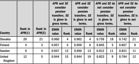
Slovakia 20 21 0.960 4 0.962 4 0.759 18 0.742 21

Finland 4 3 0.957 5 0.959 6 0.845 5 0.857 6

Sweden 9 4 0.947 13 0.950 13 0.812 11 0.831 11

United Kingdom

12 5 0.944 15 0.944 19 0.823 9 0.794 12

Source: Authors' own calculation based on Eurostat, 2018.

Table 1b.Spearman correlations of stochastic frontier estimates for the Debreu-Farrell rate (ENHN) to reach APRdepending on whether pension transfers and/or the existence of taxation in social expenditure are considered

APR(1) APR(2) ENHN (11) ENHN (12) ENHN (21) ENHN (22)

APR(1) 1

APR(2) 0.578*** 1

ENHN (11) 0.758*** 0.523*** 1

ENHN (12) 0.712*** 0.491*** 0.986*** 1

ENHN (21) 0.317* 0.806*** 0.549*** 0.539*** 1

ENHN (22) 0.345* 0.768*** 0.532*** 0.579*** 0.905*** 1

Note:APR(1) considers pension transfers whereasAPR(2) does not.

ENHN (11):APRandSEinclude pension transfers.SEis given in gross terms.

ENHN (12):APRandSEinclude pension transfers.SEis given in net terms.

ENHN (21):APRandSEdo not include pension transfers.SEis given in gross terms.

ENHN (22):APRandSEdo not include pension transfers.SEis given in net terms.

Source:Authors' own calculation based on Eurostat, 2018.

(7)

poverty threshold remain unchanged (it is as if some tax receipts are thrown into the sea; also, while the transfers are eliminated, the median household income does not change); secondly, as transfers are not supposed to have any behavioural effect,APRandAGRdo not take into account any behavioural impacts and tax money is not redirected to other policy objectives.

In this paper, we evaluate the efficiency of social public expenditure (SE) quantified over GDP³. SEincludes: social benefits, which consist of transfers in cash or kind to households and individuals to relieve them of the burden of a defined set of risks or needs; administration costs, which represent the costs charged to the scheme for its management and administration; and other expenditure, including miscellaneous expenditure by social protection schemes (e.g. the payment of property income).SEincludes pensions when we evaluateAPR(1) andAGR(1) but does not include them when we evaluate its performance in reachingAPR(2) andAGR(2). Similarly, we evaluateSE performance in both gross and net terms (i.e. bearing in mind that a part of social transfers returns to the state via taxation). We obtained grossSEon GDP (SE(1)) directly from the EUROSTAT series. However, to obtain netSEon GDP (SE(2)) we must use the series of its value in euros and the series of GDP. To subtract pensions fromSE, we use the proportion that the EUROSTAT series impute to pension benefits within all social expenditure. We have not used“in cash” social expenditures exclusively because spending on social services sometimes has an indirect impact on monetary poverty/inequality outcomes. For example, sickness or old age services in kind make it easier for citizens to strike a balance between their full-time jobs or education and their family circumstances. We have also checked that the correlations between in-cash social expenditures and APR(1) and alsoAGR(1) are weaker than those between social expenditures as a whole and the reduction in poverty and income inequality. In thefirst case, the correlations are above 0.4 but when we include services in kind within social expenditure, the correlations increase to almost 0.6.

Using directly the values of APR and/or AGR to establish a hierarchy between the EU countries imply taking into account only theﬁnal result of public policy in reducing poverty and income inequality. The effort made in social policies or the value of the poverty/income distribution rate before the social transfers are not moderated. We have checked that the hierarchies corresponding to APR(1) and APR(2) have a positive and signiﬁcant correlation that, however, is far from perfect. Therefore, while some countries have a high rank inAPR(1) and a low rank in APR(2) (e.g. Greece), others, such as Cyprus, present the opposite behaviour.

However, most nations have similar positions in the hierarchy on both objectives. We can draw similar conclusions when comparing the hierarchies in AGR(1) and AGR(2). We have also found that the rankings inAPR(1) withAGR(1) and inAPR(2) withAGR(2) have a positive and signiﬁcant relationship (above 0.70). These magnitudes are greatly linked but not the same, so their empirical behaviour is similar but not identical. Although also positive and signiﬁcant, the correlations betweenAPR(2) andAGR(1) and betweenAPR(1) andAGR(2) noticeably decline.

As we expected,SE(1) has a positive and signiﬁcant relationship withAGR(1) andAPR(1) (above 0.55 in both cases). We previously found that the correlations remain practically unchanged if we considerSE(2) or whenAPRandAGRdo not include pensions.

Likewise, AGR(1) has a positive and significant relationship withGIb(1) and a positive and significant, though less intense, relationship with PIb(1). Similarly, the absolute reduction in poverty,APR(1), has a positive and significant relationship withPIb(1) and also a positive but

3It is beyond the scope of this paper to evaluate other social public policy issues such as taxation.

(8)

not significant relationship with the value of the Gini index before the social transfers. In this paper, we consider the value of the poverty/income distribution index before the social transfers as an explanatory variable of the assessed outputs of social policy (APRandAGR) together with the real input,SE. Of course, the initial situation of poverty and income inequality rates is not an input but a contextual variable. It seems logical that the reduction in poverty rates and income inequality is greater in situations where the starting value of the poverty and Gini's index is also higher. From the law of diminishing marginal returns, we can deduce that an increase in social transfers will cause a smaller decrease in the index when we start from a lower value of that index. Similarly, PIb(1) and GIb(1) are decisively influenced by the demographic and labour market situation in the evaluated state. A larger retired population implies a larger population dependent on pension benefits, while a greater unemployment rate implies a greater number of citizens with a low (or null) level of personal income.

To check the relationship betweenPIb and Gib,on the one hand, and retirement and unemployment rates, on the other, we perform several pooled data panel regressions in whichPIb and GIb are explained by the unemployment rate (UR) and, only in the case of PIb(1) and GIb(1), also by the proportion of the population aged over 65 (65yrs). The data are from 2011 to 2015 (both years included) and in these regressions the observation in a concrete year and country is considered as an individual observation (i.e, we do not use mean values). In all cases we confirm the positive and significant influence of UR and 65yrs on PIband GIb.

3. ASSESTMENT OF PUBLIC EXPENDITURE EFFICIENCY IN REDUCING POVERTY AND INCOME INEQUALITY

3.1. Deterministic and stochastic econometric productive frontiers

Following Greene (2014), two broad paradigms are used to analyse performance in production (also known in this context as efficiency): econometric methods (EMs) and DEA. Econometric modelling is based on parametric statistical techniques while DEA is based on nonparametric, linear programming methods. Both paradigms are based on an underlying construct of the efficient production frontier that relates maximal output to inputs for the decision-making unit (DMU). With EMs, the analyst defines estimates as a continuous, regular relationship that defines the frontier. With DEA, on the other hand, linear programming methods are used to fit a piecewise linear‘hull’around the data under the assumption that the hull adequately approximates the underlying frontier, and does so better as the number of observations increases. No formulation that unifies both these approaches in a single analytical framework has yet been devised.

DEA assumes that a frontier technology exists that can be described by a piecewise linear hull that envelopes the observed outcomes. Some (efficient) observations will be on the frontier while other (inefficient) observations will be inside. The technique produces a deterministic frontier that is generated by the observed data so, by construction, some individuals are‘efficient.’This is one of the fundamental differences between DEA and EMs, where only one production unit, or even none of them, may be efficient. Both paradigms are based on an underlying construct of the efficient production frontier that relates maximal output to inputs for the‘DMU’.

In this paper, we use EMs to measure the efficiency of the social policies of the EU-28 states in reducing poverty and redistributing income. The main input variable is social expenditure on GDP

(9)

(SE), which may be expressed in gross or net terms and with or without taking into account pension expenditure. As an explanatory variable we also take the ratio before paying social expenses (PIb orGIb), which can be understood as a contextual variable. Social spending performance is analysed using two alternative econometric methods that obtain with empirical data the so-called efﬁcient frontier, i.e. for each possible combination of inputs, the maximum achievable output. A review of these approaches for measuring efﬁciency can be found inGreene (2008).

We estimate a deterministic frontier using the method known as corrected least squares (COLS). Later we use a stochastic frontier method that models inefficiency as a semi-normal random variable. In both cases, we adjust for theith decision unit of the frontier value for its outputY_i^F by means of a Cobb-Douglas function:

Y_i^F¼expðb0ÞYn j¼1

X_i;j_b_j

→lnY_i^F ¼b0þXⁿ

j¼1

bjlnX_i;j (1)

whereY_i^Fis the ideal value for the output from theith economic agent,X_i5(X_i1,X_i2,. . .,X_in) is the vector of inputs consumed by theith decision unit, andb¼ ðb0;b1;b2; . . .;bnÞis the vector of parameters. Given that the ideal output is not observable, toﬁt (1a)-(1b) we take the actual value achieved by each decision unit as an observation of the output in such a way that we mustﬁt:

lnY_i¼b0þXⁿ

j¼1

bjlnX_i;jþe^F_i (2)

whereY_iis the actual output achieved by theith decision unit. Given thatY_i^F≥Y_i, the error term e^F_i must satisfyEðe^F_iÞ≤0; whereE($) is the mathematical expectation operator.

COLS assumes that errors in (2) are attributable exclusively to the inefficiency of the decision units and have no noise component, such thate^L_i ≤0. COLS was initially proposed byWinstein (1957), whileGreene (1980)showed that it is an efﬁcient method from the econometric point of view. After obtaining the COLS adjustment of the vector of coefﬁcients,bb^COLS(see e.g. Greene (1980)for the details), we can calculate the ideal value for the output of theith decision unit as Yb^F_i ¼expðbb^COLS₀ ÞQ_n

j¼1ðX_i;jÞbbCOLS

j . Finally, the Debreu-Farrell performance measure is obtained as:

ECOLS_i¼ Yi

Yb^F_i

(3) We also measure the efficiency of social expenditures using a stochastic frontier model. In this case, we assume that the error term in (2),e^F_i, can be split into two random terms. Thefirst term,v_i, quantifies noise and is modelled as conventional white noise, whereas the second factor,u_i, is due to the inefficiency of the evaluated economic units, such thate^F_i ¼ νi −u_iandu_i≥0. Therefore, (2) becomes:

lnYi¼b0þXⁿ

j¼1

bjlnXi;jþviui (4)

As is commonplace, we assume thatu_i follows a Half-Normal random variable. Given that vi∼Nð0;σ²_vÞ and ui∼N^þð0;σ²_uÞ, this model is therefore known as Normal-Half-Normal (NHN).

(10)

This method was presented inAigner et al. (1977). According toGreene (2008: 196), this is the standard modelling in empirical efficiency studies with stochastic frontiers. It is also the basis for other models with alternative modelling of the termu_i. Many empirical studies that are representative of this approach have been conducted in healthcare economics. One of thefirst of these contributions was by Wagstaff (1989), while more recent studies include Atilgan (2016) and Kwietniewski – Schrey€ogg (2018). Other areas in which the NHN model has been applied are: educational services Titus –Eagan (2016); agricultural productionCoelli (1995a); evaluation of public entities manage- mentHerrera–Pang (2012); and evaluation of corporate benefitsMajor (2003).

FollowingGreene (2008), the widespread use of the NHN stochastic frontier model is due to its easy implementation by means of the maximum likelihood method. Moreover, testing the relative importance of the two components of the error term, v_i and u_i, is a straightforward procedure. In the NHN model, the analysis of the rateλ¼^σ_σû_v is of great interest in that when λ→0, all the decision units are efficient ande^L_i is only noise, whereas whenλ→∞; the error term is due exclusively to the inefficiency of the decision units. After adjusting (4) with a maximum likelihood method, we obtain bb^F ¼b^{Max L}¼ ðb^{Max L}0 ;b^{Max L}1 ; . . .;b^{Max L}n Þ for the parameters, the estimates linked to the variancesbσ andbλ¼bσu

bσv

, and a set of errorsfbeig_i¼1_;₂_;...;_m whose mean is below zero. In fbeig_i¼1_;₂_;...;_m we have to split the white-noise component fbv_igi¼1;2;...;mand the part due to inefficiencyfbu_igi¼1;2;...;m(seeGreene (2008)for the details about decomposingfbeig_i¼1_;₂_;...;_m). To calculate subsequently the Debreu-Farrell efficiency measure, we then use only the component of the error due to inefficiency,bu_i:

ENHNi¼exp −bui

(5)

3.2. Assessing social expenditure performance in the reduction of risk of poverty (APR)

We assess the performance of the social transfer policy of the EU-28 countries in achieving absolute reduction in the rate of poverty. We consider only one input factor: social expenditure (SE). Efﬁciency analysis ofAPRwill be conducted by including pensions in social transfers (so the initial risk of poverty rate is calculated before the pension payments) but also by excluding pensions (so the rate is calculated after the pension transfers). We evaluate the efﬁciency of SE(1) and SE(2) separately, i.e. the value of transfers minus the fact that a non-negligible proportion ofSE returns to the state via taxation.

As we pointed out in Section 2, the second explanatory variable of APR (PIb) cannot be considered an ‘input’. However, we have checked that PIb is decisively determined by the proportion of retired citizens and the unemployment rate, i.e. it reﬂects the conditions of the country in which the social policies are to be applied. We, therefore, believe that it is advisable to include it in thePIbmodel since it protects us from assigning greater levels of efﬁciency to the states that start out from a high level of retired people and/or a high level of unemployment⁴.

4We also adjusted models (2) and (5) by considering the unemployment rate and the population over 65 years instead of Pib as situational variables. However, as the results of the adjustments measured from their coefﬁcient of determination are poorer, we prefer to maintainPIbas an explanatory variable. The results of adjusting (6) are available by requesting them from the corresponding author.

(11)

We modelAPR as a Cobb-Douglas function. Then, for theith country, theAPRfrontier is:

APR^F_i ¼expðb0ÞSE^b_i¹PIb^b_i²: (6) Estimates of the COLS and NHN models (2) and (4) have been calculated and in both cases, the positive significant relationships between APR with SE and PIb are confirmed. Table 1a shows only the values of the NHN estimation of the Debreu-Farrell rate (ENHN) and the hierarchy we can obtain with this indicator. Earlier, we found that the hierarchy resulting from the COLS efficient frontier is practically equal to that from ENHN and that in the case of COLS the value of the Debreu–Farrell efficiency measure presents greater variability among the countries.

We can also verify that the Battese-Coelli statistic byCoelli (1995b) leads us to accept that a signiﬁcant inefﬁciency component exists in the EU-28 countries.

When pension transfers are included in the analysis, the most efficient countries are generally those from the Visegrad group plus Ireland and Finland, while several Mediterranean countries and the Baltic Republics are the least efficient. The countries which perform better are Hungary, the Czech Republic and Ireland and those that perform less well are Italy, Spain, Latvia, and Estonia. For the Czech Republic, Poland and Slovakia, we also observe a large rise in efficiency hierarchy compared to the rank that comes from considering simplyAPR, which was shown inTable 1a.Table 1bshows that the correlation of the hierarchies that we can establish withAPR and ENHN is high and signiﬁcant since it reaches 0.70. None of the results in this paragraph depend on whetherSEis considered in gross or net terms. Note that the Spearman correlation between the Debreu-Farrell measures for efﬁciency inAPR(1) when gross and netSE are considered is 0.98.

The hierarchy of the efficiency in APR(2) correlates positively with the obtained APR(1).

Table 1b shows that the correlations between the ENHN values inAPR (1) and APR(2) are above 0.55. These correlations are not perfect and require certain nuances. It is true that some of the most efficient countries inAPR(1) are also the most efficient inAPR(2) (Ireland, Hungary and Luxemburg). However, most of the Visegrad countries no longer have a dominant hierarchy (see the Czech Republic and Slovakia). Some Nordic countries (especially Denmark) also improve their position. The weak efficiency of the group of the Mediterranean WSs is reinforced (Portugal, Greece, Spain and Italy appear among the worst ten states). Moreover, Germany is among the states with the most unproductiveSE. The Baltic republics abandon their low efficiency position inAPR(2) and are placed in the intermediate or even in the high positions (e.g.

Lithuania). The relationship between the hierarchies when considering gross and net SE are highly correlated (0.90; see Table 1b). However, certain discrepancies are observed in the rankings obtained by Croatia, the Netherlands and Poland.

3.3. Assessing social expenditure performance in the reduction of income inequality ( AGR )

In this section, we evaluate the performance of the social transfer policy of the EU-28 countries in reducing income inequality (AGR) measured by the Gini index. This efficiency analysis is conducted by considering pension benefits within social transfers and by excluding them (i.e. the initial Gini index is obtained after the pension transfers). Again, we evaluate the efficiency of grossand netSEseparately.

(12)

As in our analysis ofSEefficiency in the reduction ofAPR, the second explanatory variable of AGRis the initial situation of income inequality beforeSE (GIb)is implemented. We can present the same reasons that led us to introduce PIb to model the efficient frontier of APR. GIb is decisively influenced by demographic and labour market issues. In Section 2, we observed a significant and positive relationship between GIb,on the one hand, and the proportion of the population over 65 and the unemployment rate, on the other. We, therefore, include in our analysis the initial level of the Gini index in order to avoid erroneously assigning a higher level of efficiency to the countries that start out from a high proportion of retired people and/or a high level of unemployment.

As withAPR, we modelAGRas a Cobb-Douglas. Therefore:

AGR^F_i ¼expðb0ÞSE^b_i¹GIb^b_i² (7) COLS and NHN models (2) and (4) for (7) have been performed and in both cases, the positive and significant relationships betweenAGRwithSEand GIbare confirmed⁵.Table 2a shows the values of ENHN and the hierarchy that we can construct with this indicator. Earlier, we checked that the hierarchy resulting from the COLS efficient frontier is practically equal to that which results from ENHN, and that with COLS the value of the Debreu-Farrell efficiency measure is more dispersed among the countries. As in our analysis ofAPR, we can see that the value of the Battese – Coelli coefficient leads us to accept that a significant error term is attributable to the inefficiency.

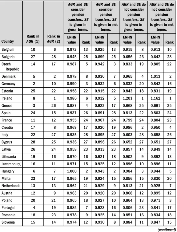
Table 2ashows that when pension transfers and gross social expenses are considered in the analysis, the states that performed better inAPR(1) also have greater values of EHNH in AGR(1), e.g. some of the Visegrad countries and Ireland. However, Germany and Sweden are among the most efﬁcient countries in AGR(1) even though they did not have an especially high EHNH in APR(1). Among the least productive states in AGR(1), some are also less productive in APR(1), e.g. the Mediterranean countries, such as Italy and Spain as well as Bulgaria. However, France is also among the states that perform poorest inAGR(1).Table 2b shows that the hierarchy resulting from considering net expenses,SE(2) is highly correlated with that corresponding to using as inputSE(1). However, in some cases, consideringSE(1) or SE(2) can lead to changes in the efﬁciency ranking. For example, consideringSE(2) (or SE(1)) implies notable decreases (increases) for Greece, Portugal and the United Kingdom (Slovakia, Poland and the Netherlands).Table 2balso shows a high positive correlation (0.8) between AGR(1) and the value of ENHN when SE(1) is considered as an input. The correlation between the hierarchy that results from SE(2) and AGR(1) is smaller but also positive. The worsening (improvement) in the relative position in EHNH compared to when AGR(1) is applied is clear in the case of Austria and France (the Czech Republic and Slovakia).

In our evaluation of the performance ofSE(1) in achievingAGR(2),Table 2aconfirms the first (last) positions of some of the states that were also the most (least) productive in achieving AGR(1), e.g. Ireland, Sweden, the Netherlands and Hungary (Spain, Italy and Bulgaria). The correlation between ENHN inAGR(2) and ENHN inAGR(1) exceeds 0.5. However, wefind that

5We alsoﬁt the regression model (7) while considering the unemployment rate and the population over 65 instead ofGIb as the contextual variables. However, as the results of the adjustments were poorer, we prefer to retainGIbas the contextual variable. The results of adjusting (7) are available by requesting them from the corresponding author.

(13)

Table 2a.NHN estimation of the Debreu-Farrell rate (ENHN) of social expenditure in reducing income inequality

Country

Rank in AGR(1)

Rank in AGR(2)

AGRandSE consider

terms.

AGRandSEdo not consider

terms.

ENHN value Rank

Belgium 10 6 0.972 13 0.925 13 0.915 8 0.913 10

Bulgaria 27 28 0.945 25 0.899 25 0.656 26 0.642 28

Czech Republic

14 17 0.987 5 0.942 3 0.833 19 0.805 22

Denmark 5 2 0.978 8 0.930 7 0.965 4 1.013 2

Germany 2 10 0.990 3 0.932 6 0.832 20 0.842 16

Estonia 25 22 0.958 22 0.915 22 0.843 18 0.831 19

Ireland 8 1 0.986 6 0.932 5 1.201 1 1.162 1

Greece 3 26 0.987 4 0.922 17 0.668 25 0.691 25

Spain 24 15 0.937 26 0.891 28 0.813 22 0.803 24

France 11 12 0.955 24 0.907 24 0.799 24 0.804 23

Croatia 17 8 0.969 17 0.920 19 0.986 2 0.950 4

Italy 22 27 0.935 28 0.895 27 0.603 28 0.658 26

Cyprus 28 25 0.936 27 0.896 26 0.652 27 0.651 27

Latvia 26 24 0.958 23 0.913 23 0.857 14 0.849 14

Lithuania 19 16 0.970 16 0.921 18 0.902 9 0.892 13

Luxembourg 16 11 0.971 15 0.925 12 0.896 10 0.896 11

Hungary 6 7 1.000 2 0.943 2 0.984 3 0.944 5

Malta 23 17 0.965 19 0.924 15 0.856 15 0.830 20

Netherlands 13 13 0.962 21 0.929 9 0.813 21 0.925 7

Austria 12 9 0.963 20 0.920 20 0.868 12 0.895 12

Poland 20 21 0.965 18 0.927 10 0.864 13 0.971 3

Portugal 4 19 0.985 7 0.923 16 0.806 23 0.841 17

Romania 18 23 0.978 9 0.925 14 0.851 16 0.834 18

Slovenia 15 14 0.974 12 0.930 8 0.884 11 0.847 15

(continued)

(14)

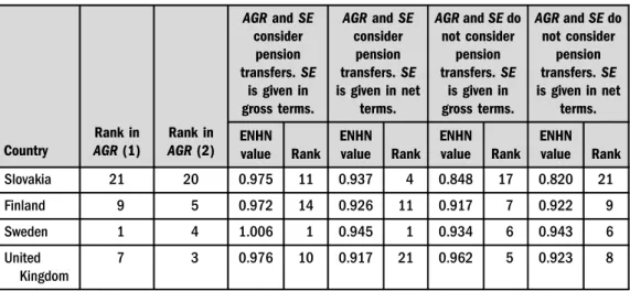
some of the Visegrad countries (except Hungary) and Germany are no longer among the most productive. The Mediterranean WSs are also reafﬁrmed as the countries whose social spending is not very productive. Greece, Italy and Spain are among the countries with the weakest performance and Portugal is one of the ten countries that performed least well. These results do not depend on whetherSEis considered in gross or net terms. Notice that the Spearman correlation Table 2a. Continued

Country

Rank in AGR(1)

Rank in AGR(2)

AGRandSE consider

terms.

ENHN value Rank

Slovakia 21 20 0.975 11 0.937 4 0.848 17 0.820 21

Finland 9 5 0.972 14 0.926 11 0.917 7 0.922 9

Sweden 1 4 1.006 1 0.945 1 0.934 6 0.943 6

United Kingdom

7 3 0.976 10 0.917 21 0.962 5 0.923 8

Table 2b.Spearman correlations of stochastic frontier estimates for the Debreu-Farrell rate (ENHN) for achieving AGRdepending on whether pension transfers and/or the existence of taxation in social expenditure are considered

AGR(1) AGR(2) ENHN (11) ENHN (12) ENHN (21) ENHN (22)

AGR(1) 1

AGR(2) 0.5489*** 1

ENHN (11) 0.8024*** 0.4714*** 1

ENHN (12) 0.5989*** 0.4457** 0.9026*** 1

ENHN (21) 0.3502** 0.8459*** 0.5653*** 0.5873*** 1

ENHN (22) 0.3989** 0.8352*** 0.5328*** 0.5992*** 0.9436*** 1

Note:APR(1) considers pension transfers whereasAPR(2) does not.

ENHN (11):APRandSEinclude pension transfers.SEis given in gross terms.

ENHN (12):APRandSEinclude pension transfers.SEis given in net terms.

ENHN (21):APRandSEdo not include pension transfers.SEis given in gross terms.

ENHN (22):APRandSEdo not include pension transfers.SEis given in net terms.

(15)

between Debreu-Farrell measures when considering gross and netSEis practically 0.95.Table 2b shows a high positive correlation (above 0.8) betweenAGR(2) and ENHN for obtainingAGR(2).

This result also does not depend on whether gross or netSEis considered. However, there is a clear loss (gain) in hierarchy when measuring the efﬁciency of spending compared to that obtained directly fromAGR(2) in Germany and France (Latvia and Poland).

4. FUZZY PATTERNS IN THE EFFICIENCY OF THE PUBLIC POLICIES IN EU- 28 FOR TREATING INEQUALITY AND POVERTY

4.1. Crisp and fuzzy k-means clustering

Cluster analysis is one of the main statistical tools for dividing a set of observations into homogeneous categories since it enables patterns in the phenomenon under the study to be identified. Conventional cluster k-means algorithms allow each element of a sample to be classiﬁed exclusively into pre-establishedK clusters. Once the number of clusters has been ﬁxed, the centroids and membership levels are determined by minimizing the dispersion of elements within a group. Fuzzyk-means algorithms relax the hypothesis that the states that the ML of an element to a group can only be full or null and assume that any observation can belong to more than one cluster with a ML bounded in [0, 1]. FollowingKlawonn et al. (2015), conventional clustering can be understood as a more general case of fuzzy clustering since fuzzy clusters can be transformed into crisp groups by considering that any observationx_i belongs exclusively to clustersif ui;s ¼max^K_k¼1ui;k, beingui;s the membership level of theith element to thekth cluster.

In classification problems related to the social sciences, the definition of classes is usually diffuse. Many of the items to be classified can participate in more than one group. If we establish two groups of countries based on their performance in AGR – i.e. ‘efﬁcient countries’ and

‘inefficient countries’ – these definitions lead us to consider the fuzzy clustering as a more realistic alternative than a hard clustering. We would accept that the memberships of Hungary in thefirst group and Italy in the second group are unequivocal. However, the Netherlands and Belgium would participate with non-negligible intensity in both the groups. This explains why fuzzy clustering analysis has been widely used in economic and social classification problems⁶. Klawonn et al. (2015)add a new reason to use the fuzzy clustering methods instead of the hard clustering methods. These authors indicate that a fuzzy clustering can help to prevent algo- rithmic problems caused by methods such as conventionalk-means clustering. The result of the conventional k-means algorithms depends strongly on the initialisation of these algorithms that sometimes lead to undesired clustering results. In fuzzy clustering this does not occur. In this sense, fuzzy clustering not only improves onk-means clustering but also provides an oppor- tunity to introduce moreflexible and sophisticated clustering models than the simple k-means algorithm while avoiding the problem of undesired clustering results.

6Derrig–Ostaszewski (1995)classified several municipalities of the State of Massachusetts based on the variables related to auto insurance fraud;Costea–Bleotu (2012)applied fuzzy clustering to distinguish between the Romanianfinancial institutions based on theirfinancial results andQuah (2014) analysed economic cycles from the fuzzy clustering perspective.

(16)

An important issue in the fuzzy k-means analysis is the optimal number of clusters. As Wang – Zhang (2007) showed, this topic has generated a great deal of attention in the literature. In this paper, we use two indices to validate the number of clusters. Theﬁrst one uses only the MLs of the elements and is a reﬁnement on Bezdek's classic index (1981) presented byDave (1996). We call this index IDB (Index by Dave–Bezdek). The second index is proposed by Xie – Beni (1991). According to Wang – Zhang (2007), this index is more complete than the one presented byDave (1996) since it uses MLs and the value of the observations. This index that we denote as IXB states that the optimal value for the number of clustersKmust minimize the dispersion within the classes and at the same time maximize the dispersion between the classes.

4.2. Fuzzy patterns in the size and efficiency of social expenditure

We now identify patterns in the EU-28 countries while taking into account two dimensions: the volume of their social expenditure (which can be considered a proxy for the size of their welfare states) and their efficiency in reducing risk of poverty and income inequality. The first variable is measured as gross social expenditure,SE(1), while performance in reducing poverty risk and income inequality is quantified by ENHN. We conduct the following three cluster analyses. First, we grouped the countries by taking into account their volume of social spending and efficiency in APR and considering both measures of it, i.e.APR(1) andAPR(2). This analysis is denoted as SE-APR. Then we conduct a similar cluster analysis by considering the efficiency of SEinAGR(1) andAGR(2) (denoted as SE-AGR analysis). Finally, we conduct a third cluster analysis by considering the volume of social spending and ENHN inAPRandAGRas discriminant variables. In all cases we useSE(1), i.e. gross social transfers with and without considering pension benefits, since EHNH values are linked to the use ofSE(1) for achievingAPR(1),APR(2),AGR(1) andAGR(2). To reduce the length of the paper it only shows the table with the results of the third cluster analysis. Of course, numerical results supporting the comments on SE-APR and SE-AGR analyses are available to the reader.

To implement the cluster algorithm, we consider the standardized values of all variables. As Yu et al. (2012) suggested, to set the number of clusters we start with a maximum number

ffiffiffin p ¼ ffiffiffiffiffi

p28

≈5 and a minimum of 2. We also usem52, as empirical applications usually do.

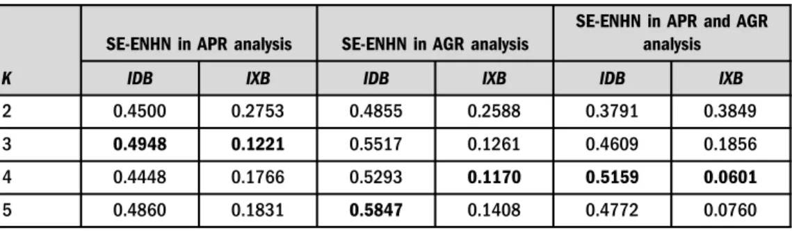
The values of IBX and IDB inTable 3enable us to identify the best partition.

Table 3. Values of IDB and IXB

SE-ENHN in APR analysis SE-ENHN in AGR analysis

SE-ENHN in APR and AGR analysis

K IDB IXB IDB IXB IDB IXB

2 0.4500 0.2753 0.4855 0.2588 0.3791 0.3849

3 0.4948 0.1221 0.5517 0.1261 0.4609 0.1856

4 0.4448 0.1766 0.5293 0.1170 0.5159 0.0601

5 0.4860 0.1831 0.5847 0.1408 0.4772 0.0760

Note: Bold indicates the optimum value of IDB and IXB indexes.

Source: Author's own calculation based on Eurostat, 2018.

(17)

4.2.1. Patterns in the volume and efficiency of social expenditure in reducing the risk of poverty rate.Table 3shows that the values of IDB and IXB suggest taking k53 in SE-APR cluster analysis. In this case, thefirst cluster is characterized by much higherSElevels than the EU-28 average and ENHN values that are also clearly above the EU-28 average. Practically all the countries in the first cluster are EU-15 countries whose MLs are above 0.5 (Belgium, Denmark, Finland, France, Luxembourg, Austria, Sweden and the United Kingdom). Only one non-EU-15 country (Slovenia) is clearly within this group. Spain has a significant but secondary ML in this group (0.32). We could also consider Ireland to be a member of this group, but its ML does not reach 0.5. Ireland's low SElevel also puts it in the third group, the main characteristics of which are a lower social expenditure level and a higherSEefficiency. We could also consider Hungary and Croatia to be members of this group, though their levels are lower than those of Ireland.

The second cluster comprises nations whose SE is heterogeneous but whose average is slightly higher than that of the EU-28. The main characteristic of the countries in this group is their low ENHN in APR. All these countries are either the Mediterranean WSs (Italy, Spain, Greece and Portugal) or, surprisingly, the continental WSs, e.g. Germany and the Netherlands (whose ML are above 0.6) and France (0.36). Also, in this group there are several Eastern Europe countries, such as Bulgaria (0.47) and Romania (0.25), as well as Cyprus (0.49).

TheSEof countries in the third cluster are below the EU-28 average but their ENHN inAPR are clearly above the average. In this group there are Eastern European countries, such as those of the Visegrad group (Hungary, Czech Republic, Poland and Slovakia) and the Baltic republics, and these countries usually have a clear intensity (above 0.7). Other Eastern European countries are also members of this group (Croatia, Romania and Bulgaria) but their intensity is lower. Also belonging to this group but with lower signiﬁcant MLs are Malta, Luxembourg and Ireland, which are from completely different cultural and geographical areas.

In conclusion, we have identified a first group made up of most of the EU-15 countries regardless of their welfare model (the Nordic countries, the continental European countries and the Anglo-Saxon countries). The second group comprises the countries with the poorest ENHN, e.g. the Mediterranean WSs, the continental WSs, such as Germany and the Netherlands, and, less clearly, France. Bulgaria, Romania and Cyprus may also be considered to belong to this group. The third group is basically made up of the non-EU-15 countries, especially the Visegrad states and the Baltic Republics. Luxembourg and Ireland also have a significant membership level for this group.

4.2.2. Patterns in the volume and efficiency of social expenditure in reducing income inequality.In SE-AGR cluster analysis, IDB recommends establishing five clusters, while IXB recommends four (seeTable 3). Wang–Zhang (2007) indicate that indices, which combine sample values with MLs, are more robust. Following the IXB criterion, therefore, in our analysis we identify four clusters.

Essentially, the first cluster comprises the same countries as the first cluster in our SE-APR analysis and has similar characteristics. The countries in this group have much higherSElevels than the EU-28 average, while the mean ENHN inAGRis slightly above the average. Practically all members of this cluster are the EU-15 countries (Belgium, Denmark, Germany, the Netherlands, Austria and the United Kingdom). Due to its low efﬁciency inAGR(0.66), France does not clearly belong to this group. We also see that Slovenia, Luxembourg and two classic

(18)

Mediterranean WSs (Portugal and Spain) have a non-negligible ML that, nevertheless, is below 0.5.

The main characteristic of the second group is that theSEs are the lowest of the EU-28. On the other hand, the efﬁciency of the countries in this group, despite being below the EU-28 average, is not the lowest and is highly heterogeneous. The main characteristic of one group (the fourth) is the low ENHN for AGR. The Baltic nations, the CEE countries, such as Poland, Romania, Slovakia and the Czech Republic, and Malta are very close to this group. Luxembourg also has a non-negligible ML to this group.

The composition of the third cluster is similar to that of the third cluster in our SE-APR analysis. Members of this group have a slightly lowerSEthan the EU-28 but a high ENHN in AGR. Hungary, Croatia and Ireland are undoubtedly within this group. Surprisingly, Sweden remains in this group with some intensity due to its high performance inAGR. Luxembourg and the Czech Republic have a signiﬁcant ML for this group due to theirSElevel, whichﬁts in the group standard. Similarly, Slovenia presents a non-negligible presence (but clearly below 0.5) in this group.

The fourth group comprises countries with very heterogeneousSElevels that, as a common denominator, have very low efﬁciency inAGR. The countries that clearly belong to this group are Bulgaria, Italy, Greece and Cyprus. Portugal, Spain and France also exhibit a signiﬁcant ML (but never above 0.5) in this group because of their poor ENHN inAGR.

We have identified a first group that comprises most of the EU-15 countries except the Mediterranean ones (in this group, Italy and Greece are not included at all and Spain and Portugal are included only partially). The second group basically comprises the Eastern and Central European states and the Baltic countries. The main characteristic of these countries is their low SElevel. The third group, which is highly efﬁcient in reducing income inequality, is made up of a heterogeneous set of countries (culturally and geographically speaking). The fourth group, which has the lowestAGRperformance, is made up of countries normally considered as the Mediterranean-type WSs and Bulgaria.

4.2.3. Patterns in the volume and efficiency of social expenditure for reducing both risk of poverty and income inequality. We now present the results of a cluster analysis that in- corporates ENHN in bothAPRandAGR. In this way we consider the efficiency ofSE(in gross terms) in relation to both objectives. We incorporate efficiency measures for developing poverty and income inequality reduction policies without computing the pension transfers. Table 3 shows that IDB and IBX both recommendfitting four clusters.Table 4shows the level at which each country belongs to each cluster and the standardized values ofSEand ENHN inAGRand APR.As we indicate below, these groups correspond clearly to the groups that were identified in the SE-AGR analysis.

Essentially, the first group is the same first group as identified in the previous cluster analyses. The countries in this group have a much higherSElevel than the EU-28 average, while the ENHN inAPR and AGRare average for the EU-28. Belgium, Denmark, France, Austria, the United Kingdom and Slovenia are clearly in this group. Due to their efﬁciency inAPR, Germany and Holland have membership levels that do not exceed 0.5, but this group is still their natural cluster. Luxembourg has ENHN values inAGRandAPRthat justify its inclusion in this group with a signiﬁcant intensity though this is clearly below 0.5. Practically every country in this

(19)

Country

ENHN in APR(1)

ENHN in APR(2)

ENHN in AGR(1)

ENHN in AGR(2)

SE(1) including pensions

SE(1) without including pensions

ML in

Group 1 ML in

Group 2 ML in

Group 3 ML in Group 4

Belgium 0.095 0.025 0.120 0.482 1.048 1.347 0.92 0.03 0.03 0.02

Bulgaria 1.476 1.059 1.369 1.685 0.888 0.680 0.06 0.16 0.04 0.73

Czech Republic

2.007 0.114 0.941 0.206 0.691 0.105 0.12 0.69 0.12 0.06

Denmark 0.521 0.678 0.487 0.903 1.474 0.913 0.81 0.05 0.11 0.03

Germany 0.322 1.113 1.133 0.215 0.851 0.999 0.42 0.18 0.10 0.30

Estonia 1.639 0.189 0.653 0.119 1.446 1.200 0.03 0.88 0.04 0.05

Ireland 1.247 2.639 0.899 2.876 0.544 0.923 0.20 0.14 0.59 0.07

Greece 0.405 2.098 0.946 1.587 0.342 0.986 0.04 0.06 0.02 0.88

Spain 1.557 0.520 1.838 0.375 0.244 0.317 0.23 0.24 0.08 0.46

France 0.488 0.559 0.821 0.486 1.704 1.535 0.53 0.13 0.10 0.24

Croatia 0.611 0.950 0.023 1.076 0.380 0.210 0.11 0.12 0.74 0.03

Italy 1.237 2.127 1.946 2.128 0.982 0.588 0.08 0.10 0.04 0.78

Cyprus 0.991 0.108 1.897 1.722 0.150 0.172 0.13 0.20 0.07 0.59

Latvia 1.077 0.017 0.689 0.007 1.545 1.522 0.04 0.87 0.05 0.05

Lithuania 0.484 0.720 0.023 0.371 1.512 0.972 0.08 0.67 0.19 0.05

Luxembourg 0.842 0.939 0.045 0.327 0.199 0.122 0.27 0.21 0.47 0.05

Hungary 2.214 1.452 1.714 1.061 0.659 0.071 0.02 0.02 0.96 0.00

Malta 0.462 0.078 0.296 0.016 0.938 0.410 0.02 0.95 0.02 0.02

Netherlands 0.329 0.505 0.459 0.372 1.146 0.274 0.47 0.18 0.09 0.25

(continued)

mica70(2020)1,37-6155

(20)

Country

ENHN in APR(1)

ENHN in APR(2)

ENHN in AGR(1)

ENHN in AGR(2)

SE(1) including pensions

SE(1) without including pensions

ML in

Group 1 ML in

Group 2 ML in

Group 3 ML in Group 4

Austria 0.620 0.454 0.365 0.090 0.999 0.237 0.85 0.06 0.06 0.03

Poland 0.282 0.064 0.255 0.054 0.790 2.028 0.01 0.97 0.01 0.01

Portugal 0.373 0.765 0.828 0.427 0.490 0.661 0.25 0.32 0.09 0.35

Romania 0.379 0.957 0.465 0.053 1.495 1.411 0.08 0.70 0.08 0.14

Slovenia 0.669 0.516 0.254 0.221 0.030 0.659 0.55 0.18 0.21 0.06

Slovakia 1.074 0.135 0.302 0.080 0.888 0.424 0.02 0.93 0.02 0.02

Finland 0.875 0.741 0.111 0.498 1.310 1.269 0.85 0.04 0.08 0.03

Sweden 0.065 0.409 2.011 0.640 0.933 1.171 0.90 0.03 0.06 0.02

United Kingdom

0.124 0.515 0.332 0.879 0.572 1.737 0.89 0.03 0.06 0.02

Note: SE and ENHN values are standardised.

In bold membership levels greater than 0.4 are outlined and in italic are outlined membership levels above 0.15 but below 0.4.

Source: Author's own calculation based on Eurostat, 2018. ActaOeconomica70(2020)1,37-61

(21)

cluster is from the EU-15. However, no Mediterranean country has this group as a main cluster.

Notice that the MLs of Spain and Portugal to this group are below 0.25.

The second group essentially comprises the same countries as those in the second group of our SE-AGR cluster analysis, i.e. basically, the former Communists countries. The main characteristic of this group is that its members have the lowestSE, which is usually accompanied by efﬁciency inAPRand/orAGRbelow the UE-28 average. The Czech Republic, Slovakia, Estonia, Latvia, Lithuania, Malta, Poland and Romania have MLs of 0.6 or higher in this group. Bulgaria and Luxembourg are included here with a membership level of around 0.2 due to their lowSE.

However, the poor (great)SEperformance of Bulgaria (Luxembourg) more clearly justiﬁes its inclusion in the fourth (third) group.

The third group is similar to the group 3 in the above cluster analyses. Countries in this group have a substantially lowerSEthan the EU-28 average but high efﬁciency in social policies.

Hungary, Ireland, Croatia and Luxemburg are clearly members of this group. Slovenia is also included in this group, but with a lower intensity.

The fourth group is similar to the fourth cluster in our SE-AGR analysis. It is highly heterogeneous in terms of the effort made in social expenditure. Its main characteristic is the low ENHN values. Spain, Italy, Greece, Bulgaria and Cyprus are the members with the highest MLs.

Another Mediterranean country, Portugal, has a significant ML for this group (0.35). The secondary presence of the Netherlands and Germany (France) is justified by their low performance in achievingAPR(AGR).

5. CONCLUSIONS

We have applied two econometric methods to measure the efficiency of social spending in the reduction of poverty and inequality:corrected ordinary least squares and normal-half normal stochastic frontier. Both methods yield practically identical results. To simplify the presentation of these results, we show only those obtained with the latter method. Our analysis of the reduction in risk of poverty when all types of social expenditures are taken into account shows that the worst-off countries are the Baltic republics and the southern European countries, such as Bulgaria, Italy and Spain. The highest productivities, on the other hand, are observed in the countries of the Visegrad group and Ireland. Not considering pension expenditure shows a hierarchy with a positive and signiﬁcant correlation than the results when pensions are included.

However, some of the Visegrad countries disappear from the group with the best performance and the Baltics republics cease to belong to the group of countries with the lowest efﬁciency. On the other hand, all Mediterranean countries and Germany are added. Considering net SE rather than gross SE does not lead to substantial changes in the hierarchies for efﬁciency relating to risk-of-poverty reduction.

When we evaluated the performance of social expenditure in reducing income inequality, we found that the best- and worst-ranked countries are essentially the same as in our analysis of risk-of-poverty reduction. However, this statement should be nuanced since we also found that some EU-15 countries, e.g. Sweden, Hungary, Luxembourg and Ireland, are now among the most efficient while the SEs of France and the southern European countries are less productive.

In a fairly robust way, we found that the countries whose welfare systems (WSs) are commonly considered Nordic or Continental are kept together in the same group (i.e. the first).

(22)

Also, Slovenia belongs to this group quite consistently. We also identified a second group made up of states that joined the EU after 2000 and have low levels of social expenditure and heterogeneous SE efficiency, e.g. the Baltic Republics and several Visegrad countries. The Classical Mediterranean WSs (Italy, Greece, Portugal and Spain) form a group with Cyprus and Bulgaria.

Their SE level is heterogeneous but their social expenditure efficiency is very low. With regard to the Anglo-Saxon countries, the United Kingdom belongs to the first group while Ireland, along with Luxembourg (which theoretically belongs to the continental WS model), Hungary and Croatia, is a member of a group whose social expenditure has the greatest efficiency of all the EU-28 countries.

Fuzzy cluster analysis enables us to capture the complexity of the panorama of the size and efficiency of social expenditure in the EU-28. It reveals the ambiguity of some countries when it comes to classifying them into identified patterns. We conclude, therefore, with the following remarks. France (Germany, the Netherlands) were included essentially in the first group but their low efficiency in reducing income inequality (risk of poverty) puts them in the group of the

‘Mediterranean’countries (i.e. the fourth). In the same cluster analysis, Luxemburg and Ireland are included in the group of the countries that perform better at reducing poverty indices (i.e.

the third) but also in the main group for the EU-15 countries. We also detect ambiguity for Slovenia. This country is mainly identified as a member of the‘first’cluster but it also belongs to the group of the countries whose social spending is highly productive. On the other hand, fuzzy clustering classifies Belgium, Slovakia, Hungary and Italy unequivocally to one group.

ACKNOWLEDGEMENTS

The authors acknowledge invaluable comments on a previous version of this paper from two anonymous reviewers.

REFERENCES

Aigner, D. Lovell, C. K. Schmidt, P. (1977): Formulation and Estimation of Stochastic Frontier Production Function Models.Journal of Econometrics, 6(1): 21–37.

Afonso, A. Aubyn, M. S. (2004): Non-Parametric Approaches to Education and Health Expenditure Efﬁciency in OECD Countries.Journal of Applied Economics, 8(2): 227–246.

Afonso, A.Aubyn, M. S. (2006): Cross-Country Efﬁciency of Secondary Education Provision: A Semi- Parametric Analysis with Non-Discretionary Inputs.Economic Modelling, 23(3): 476–491.

Afonso, A.Schuknecht, L.Tanzi, V. (2010): Income Distribution Determinants and Public Spending Efﬁciency.The Journal of Economic Inequality, 8(3): 367–389.

Anker, J. Linden, J.– Hauge-Wegner, M. Holch, J. A. (2009): Overview and Analysis. Minimum Income Schemes in Denmark: A Study of National Policies.Brussels: European Commission.

Atilgan, E. (2016): Stochastic Frontier Analysis of Hospital Efﬁciency: Does the Model Speciﬁcation Matter?

Journal of Business Economics and Finance, 5(1): 17–26.

Atkinson, A. (2000): A European Social Agenda: Poverty Benchmarking and Social Transfers.Euromod Working Paper, No. EM 3/00.

(23)

Arts, W. A.Gelissen, J. (2010): Models of the Welfare State. In: Castles, F. G.Leibfried, S.Lewis, J.

Obinger, H.Pierson, Ch. (eds):The Oxford Handbook of the Welfare State. Oxford: Oxford Uni- versity Press, pp. 569–583.

Beblo, M. Knaus, T. (2001): Measuring Income Inequality in Euroland. The Review of Income and Wealth,47: 301–320.

Bezdek, J. C. (1981):Pattern Recognition with Fuzzy Objective Function Algorithms.Boston: Springer.

Bogdanov, G.Zahariev, B. (2009):Analysis of the Situation in Relation to Minimum Income Schemes in Bulgaria. A Study of National Policies. Brussels: European Commission.

Bradbury, B.J€antti, M. (2001): Child Poverty across Twenty-Five Countries. In: Bradbury, B.Jenkins, S. Micklewright, J. (eds):The Dynamics of Child Poverty in Industrialised Countries. Cambridge University Press, pp. 62–91.

Cantillon, B.Vandenbroucke, F. (2014):Reconciling Work and Poverty Reduction: How Successful are European Welfare States?Oxford: Oxford University Press.

Cantillon, B.Marx, I.–Van den Bosch, K. (1997):The Challenge of Poverty and Social Exclusion. To- wards 2000: The New Social Policy Agenda.Paris: OECD.

Cantillon, B.Marx, I.Van den Bosch, K. (2002): The Puzzle of Egalitarianism: About the Relationships between Employment, Wage Inequality, Social Expenditures and Poverty.Working Papers, No. 337, Luxembourg Income Study.

Cincinnato, S. Nicaise, I. (2009):Minimum Income Schemes: Panorama and Assessment. A Study of National Policies (Belgium).Brussels: European Commission.

Coelli, T. J. (1995a): Recent Developments in Frontier Modelling and Efﬁciency Measurement.Australian Journal of Agricultural and Resource Economics, 39(3): 219–245.

Coelli, T. J. (1995b): Estimators and Hypothesis Tests for a Stochastic Frontier Function: A Monte Carlo Analysis.Journal of Efﬁciency Analysis, 6(3): 247–268.

Cook, L. (2010): Eastern Europe and Russia. In: Castles, F. G. Leibfried, S. Lewis, J. Obinger, H.

Pierson, Ch. (eds):The Oxford Handbook of the Welfare State. Oxford: Oxford University Press, pp. 671–686.

Clements, B. (2002): How Efﬁcient is Education Spending in Europe?European Review of Economics and Finance, 1(1): 3–26.

Costea, A.–Bleotu, V. (2012): A New Fuzzy Clustering Algorithm for Evaluating the Performance of Non- Banking Financial Institutions in Romania.Economic Computation and Economic Cybernetics Studies and Research, 46(4): 179–199.

Dave, R. N. (1996): Validating Fuzzy Partitions Obtained Through C-Shells Clustering.Pattern Recognition Letters, 17(6): 613–623.

Derrig, R. A.–Ostaszewski, K. M. (1995): Fuzzy Techniques of Pattern Recognition in Risk and Claim Classiﬁcation.Journal of Risk and Insurance: 447–482.

Esping-Andersen, G. (1990):Three Worlds of Welfare Capitalism. Cambridge: Cambridge Policy Press.

Ferrera, M. (2005): Welfare States and Social Safety Nets in Southern Europe: An Introduction. In: Ferrera, M. (ed.):Welfare State Reform in Southern Europe. Fighting Poverty and Social Exclusion in Italy, Spain, Portugal and Greece. Abingdon: Routledge, pp. 1–23.

Finn, D. Schulte, B. Eichhors, O. Kaufmann, O. Konle-Seidl, R. (2008): Employment First’:

Activating the British Welfare State. Bringing the Jobless into Work? Experiences with Activation Schemes in Europe and the US. Berlin: Springer.

Greene, W. H. (1980): Maximum Likelihood Estimation of Econometric Frontier Functions.Journal of Econometrics, 13(1): 27–56.