Comparative Analysis
of the Economic Development Paths of Hungarian Counties
György Kocziszky
University of Miskolc regkagye@uni-miskolc.hu
Dóra szendi
University of Miskolc regszdor@uni-miskolc.hu
summary
The literature has analysed economic growth issues for nearly 250 years, and formulated theories, indicators and calculations. The same cannot be observed for economic development. This is reflected, among others, by the fact that some publications still use the terms economic growth and development synonymously. In the present study, the authors, after a brief theoretical overview of economic development and path dependency, quantified the economic development of 19 Hungarian counties and the capital city using a complex index, and then examined the changes in the index between 1995 and 2019. The final part of the paper analyses the expected similarities and differences in the development paths up to 2024. The counties have followed different development paths over the last 25 years, a trend that is also reflected over the forecast horizon. The development trajectories of the counties are more sensitive to shocks than the paths of specific GDP output, due to global, macro and local shocks that occur from time to time.
Keywords: development path, path dependency, value system, ex-post and ex-ante analysis, simulation
JEL codes: o10, R12
DoI: https://doi.org/10.35551/PFQ_2021_s_2_1
R
Research in development theory became a focus of interest after World War II, mainly in the context of the socio-economic situation of countries liberated from colonial rule and the opportunities of poor countries to catch up.A number of complementary and clarifying explanations have been put forward on the causes of development and their role. Despite this (or perhaps because of it), there is still no uniform, universally accepted method of measuring development. All authors agree, however, that it is a complex concept, that is, it does not only express the increase in material goods, but also the development of a community and that quality of life plays a decisive role in assessing the process of development (Pike et al. 2006, p. 7; szentes, 2011, p. 24; Gingale, 2017, p. 15; Kocziszky, 2008, p. 10; Benedek, 2010, p. 8).
Economic development is therefore more and qualitatively different (higher education, longer life expectancy in good health, etc.) from expanding output. In addition to examining the uneven development of the world economy, regional economic research has focused on differences in development within a national economy.
What could explain this?
on the one hand, economic growth is an important but not sufficient condition for development. Even with rapid growth, economic development can be more moderate, and even modest output growth can induce greater improvements in quality of life.
This is true at the meso level as well, as a number of empirical studies have shown.
The concentration of economic activity (agglomeration effect) resulting in higher output (GDP) in some regions than the national average and lower output (GDP) in other regions does not automatically imply that the same difference in quality of life is created between the two regions.
on the other hand, we still have only an
approximate, vague idea of the extent to which differences in development are tolerated in a given society. Tolerance of this difference is not independent of the value system of the community concerned. crossing the threshold can trigger societal discontent and create a level of disconnection that is extremely slow to recover, if at all, in the short to medium term.
Thirdly, government interventions to reduce disparities and achieve convergence seem to have limited results.
Fourthly, there is a risk of a development trap developing once the above thresholds are crossed. Differences in quality of life affect the various age groups and educational levels differently. Those with a higher education level and a desire for a better quality of life leave such areas, while those who stay put find it harder to meet the demands of creative destruction.
Regional economic growth is a positive sign of change in the specific output of a given territorial unit. By contrast, territorial economic development is a change in the way in which the economic, infrastructural, cultural, environmental and social factors that determine the quality of life of the inhabitants of a given area result in a better than before satisfaction of the needs and well-being of the inhabitants. Development therefore means a qualitative change.
In the 20th century, four main schools of thought (economic history, sociology, institutional economics and geography) shaped the understanding of territorial development (see Table 1).
It is a merit of the economic history school to recognise that evolution is not linear, but changes levels from time to time as a result of the division of labour (Ricardo, 1816), industrialisation (Rostow, 1960) and innovation.
The representatives of the sociological school have included many intangible elements in their explanations. The famous puritan
theory of Max Weber (1924) emphasises the importance of frugality, thrift, hard work, discipline and commitment to learning as factors generating development.
The dependency theory (Wallerstein, 2010) argues that less developed regions (countries) become dependent and trapped in the current world system by capital from more developed regions, and therefore do not choose a development path that is appropriate to their own capabilities.
Kopátsy goes even further when he argues that one cannot talk about development without taking culture and behaviour into account, and criticises mainstream economics for not considering these soft factors as influencing development (Kopátsy, 2011).
Amartya Sen (1987) associated development with the freedom to act and the freedom of choice. He criticises the technocratic approach to economic activity (by what means a given goal can be achieved), and emphasises ethical Table 1 Theories explaining regional developmenT
serial
no. school hypothesis representatives
1. School of economic history (state models)
Development is induced by changes in social and economic structure (primary, secondary, tertiary sectors)
Rostow (1960) Clark (2007)
Development is determined by industry and social and mental change
Rostow (1960)
Abrupt changes in basic innovations determine economic and social development
Schumpeter (1934)
2. School of sociology (behavioral sciences)
Puritan behaviour (protestant ethics) and religion influence development
Weber (1924)
Freedom, the end of exploitation generates development
Parsons/Neil (1984)
Local commitment and traditions of civilisation release surplus human ‘energies’
Kopátsy, S. (2011)
Dependency theory Wallerstein (2010)
3. Institutional economics A rationally functioning institutional system generates development
North (1990) Ackermann (2001) 4. Geographical theories New economic geography: agglomeration advantages
induce development
Krugman (1997)
The geographical location of a given region influences development
Sachs–Mellinger–Gallup (1999)
Evolutionary changes lead to non-linear development Sahlins (1997)
Lengyel–Bajmóczy (2013) Source: own editing
considerations because economic activities should serve well-being (sen, 1987).
Institutional economists ask the question of what kind of institutional system, or to what extent a more developed institutional system contributes to the social and economic development of regions. In this context, North stresses that the adoption of formal rules (legislation) and norms of behaviour applied in more developed regions does not necessarily imply the same level of development for different cognitive and mental reasons (North, 1990).
Geographical theories seek to explain the impact on development of the spatial location of economic sectors and networks, the evolution of institutions, and the convergence or divergence of spatial systems. New economic geography emphasises the endogenous nature of local factors in the context of development (Krugman, 1997). others link development to geographical location (sachs, Mellinger, Gallup, 1999) and to the competitiveness of the region. Evolutionary economic geography rejects the rationalist theses of neoclassical economics of perfect information and general equilibrium (Boschma, Lambooy, 1999;
spahn, 2020), emphasising instead the impact of constant technological change and the effect of its endogenisation on development (Lengyel, Bajmóczy, 2013). It offers an explanation for the spatial evolution of sectors and networks, the evolution of institutions and spatial systems.
According to evolutionary development theory, once exogenous shocks (e.g. pandemics) have passed, the development path of a region does not necessarily return to the original trajectory, but can follow a steeper trajectory due to its stronger capacity for renewal. (of course, it is debatable how long this new trajectory lasts, whether endogenous shocks occur that could trigger a new developmental break.)
The aim of our research:
• to set up an econometric model suitable
for studying regional development paths,
• to conduct empirical studies for 19 Hungarian territorial units (counties), to determine the value of the aggregate development index ex post (1995-2020) and ex ante (2021-2024),
• comparative analysis of results, drawing conclusions.
MoDEL AND INDICAToRS FoR ThE ANALySIS
The model
In setting up our model, we assumed that the development path of a territorial unit is influenced by both the path dependence (North, 2005) and the factors linked to the value system of society and their changes (trajectory formation, Mccloskey, 2016).
The model considers both exogenous (macro-level) and endogenous (meso-level) influences (Figure 1).
Description of inputs
■ Regional knowledge intensity (KII) We hypothesise that knowledge intensity (i.e.
willingness to learn, education and R&D background, as well as innovative milieu) has a strong impact on the quality of life of the people living in a region and on the development of the region in several aspects, as evidenced by the literature (camagni, 1991;
MacKinnon et.al., 2002; Kocziszky, Benedek, 2012; Kocziszky, szendi, 2018).
In our model, changes in knowledge intensity are the result of the interaction of four factors:
δKIi(t) = β1δGDP(t)+α1δRDi(t)+α2δHEi(t)+ε(t) (1) Where,
δ: percentage change (year/year), GDP: macro GDP,
RD: research and development expenditure of the region,
HE: population of the region in higher education per 10,000 inhabitants,
i: serial number of the territorial unit under study,
ε: error term,
t: time span of the forecast, α, β: estimated parameters.
■ Demographic characteristics (DEI) In our forecasting model, we estimated the activity rate by examining changes in fertility, ageing and mortality indices:
δARi(t)=α4 δÖIi(t)+α5δHIi(t)+α6δTi(t)+εt (2) Where,
δ: percentage change (year/year),
ÖI: ageing index, HI: mortality index, T: fertility index, ε: error term,
t: time span of the forecast, α: estimated parameter.
We hypothesise that the size of the activity rate has an impact on, among other things, the employment rate, the gross public debt to GDP ratio, the knowledge intensity of the region, and the specific regional output.
■ sectoral structure (SECT)
The structure of the region's economy has an impact on the dynamism of the economy. A recovery is indicated by an increase in the number of new and industry 4.0 related businesses.
The sectoral structure is particularly relevant given that one of the causes of the economic Figure 1 logical sTrucTure of The analysis
Source: own editing
• Economic performance (7)
• Quality of the infrastructure (5)
• Income situation (5)
• Environmental condition (3)
Aggregated development index MACRO FACTORS
• GDP/capita
• Governmental debt
• Deficit of trade balance
• Inflation
SPATIAL INPUT
• Knowledge intensity (2)
• Demographic situation (4)
• Economic structure (5)
• EU and state funds (1)
recession after 1989 was the attachment to heavy industry (mining, metallurgy) and the unsuccessful attempts to revive the sector.
changes in the weight of a given sector are processed by the model according to the following relationship:
δSECTij(t)=β3δTBt+α1δRDij(t)+εt (3) Where,
δ: percentage change (year/year), TB: change in trade balance RD: R&D expenditure,
i: serial number of the territorial unit under study,
j: sector serial number, ε: error term,
t: time span of the forecast, α, β: estimated parameters.
Description of the relationships between inputs and outputs
■ Economic output of the region (GDPI) In estimating the expected size of economic output, the model takes into account the change in output of the national economy, the value added and investment of the five sectors under consideration, employment, and the equilibrium of inflation and the economy.
The form of the estimating function:
δGDPi(t)=β4δCPI(t)+β3δTB(t)+β2δGD(t)+ α7δSECTij(t)+γ2δERi(t)+γ3δURi(t)+γ4δKIi(t)+
γ5δDEi(t)+γ6δBij(t)+γ7δPUBi(t)+εt (4)
Where,
δ: percentage change (year/year), ERi: regional employment rate, URi: regional unemployment rate, CPI: inflation rate,
TB: trade balance, GD: public debt,
SECTij: value added of five sectors,
KIi: knowledge intensity of the region, DEi: demographic situation,
Bi: sectoral investment,
PUBi: number of publications per 10,000 inhabitants,
i: serial number of the territorial unit under study,
j: sector serial number, ε: error term,
t: time span of the forecast, α, β, γ: estimated parameters.
It is worth noting that there is a discrepancy between regional and national GDP per capita in terms of size, rate of change and volatility, not least because of employment rates.
■ Infrastructure situation of the region (INFI)
The provision of infrastructure is both an important element in the development of a given region and has an impact on the future development potential of the region under study (crescenzi, Rodríguez-Pose, 2012;
ottersbach, 2001; Bach et al., 1994).
six factors were included in our analysis:
δINFi(t)=β1δGDP(t)+γ8δHOUi(t)+γ9δDOCi(t)+ γ10δPDi(t)+γ11δHOSPi(t)+γ12δWATERi(t)+εt (5) Where,
δ: percentage change (year/year), GDP: macro GDP,
HOUi: change in the number of dwellings built per 10,000 inhabitants,
DOCi:change in the number of doctors per 100,000 inhabitants,
PDi: population density,
HOSPi: number of available hospital beds per 100,000 inhabitants,
WATERi: secondary utility gap, ε: error term,
i: serial number of the territorial unit under study,
t: time span of the forecast,
β, γ: estimated parameters.
The infrastructural situation/development of the region improves when the value of the sub-index increases.
■ Income situation of the region (INPI) The inclusion of the income module is mainly justified by the significant regional disparities in household income, poverty risk and youth dependency.
The estimating function considers seven factors:
δINPi(t)=β4δCPI(t)+β2δGD(t)+γ13δINCi(t)+γ14δRPi(t) +γ15δSOCi(t)+γ16δDEPi(t)+γ17δSECTi(t)+εt (6) Where,
δ: percentage change (year/year), INCi: change in household income, RPi: poverty risk in the area,
SOCi: change in the amount spent on care for the elderly,
DEPi: youth dependency ratio in the region, SECTi: economic structure of the region, CPI: inflation rate,
GD: public debt,
i: serial number of the territorial unit under study,
ε: error term,
t: time span of the forecast, β, γ: estimated parameters.
The income situation of the region improves when the value of the sub-index increases.
■ Environmental footprint of the region (EFI)
The study of the impact of economic output and income on the environment was initiated by the environmental movements that emerged in the 1950s. The various international (uN, Eu) and national documents aimed at assessing sustainability set out highly complex goals (e.g. The 2030 Agenda for sustainable Development - adopted by the 70th uN Ge-
neral Assembly - contains 17 goals and 169 sub-goals), which require 241 indicators to monitor.1 However, the available regional environmental databases are currently much more limited.
Taking this into account, our model processes environmental impacts (footprints) according to the following relationship:
δEFi(t)=γ18(δGDP(t) ⁄(δWAi(t))+γ19δGAi(t)+
γ20(δGDP(t) ⁄(δELi(t))+εt (7) Where,
δ: percentage change (year/year), GDP: macro GDP,
WAi: change in waste collected in given region,
GAi: change in the proportion of green areas in a given region,
ELi: change in electricity consumption in a given region,
ε: error term,
i: serial number of the territorial unit under study,
t: time span of the forecast, γ: estimated parameter.
Database
The literature is, to this day, still lacking a uniformly accepted measure of economic development. The only consensus is that economic, social and environmental indicators should be taken into account when measuring development, but there are different opinions on what these should be and what methodology should be used to integrate the various factors (complex index, cluster) (szűcs, Káposzta, 2018; Faluvégi, 2000). As a result, a number of indicators have emerged (e.g. the Measure of Economic Welfare = MEW; the Index of sustainable Economic Welfare = IsEW; the Genuine Progress Indicator = GPI, etc.),
which take into account other factors besides economic output (GDP). The problem is that their application is not yet integrated into the practice of statistical offices.
In measuring regional development, it was assumed that a distinction should be made, firstly, between national and meso-level factors and, secondly, between causal factors (input-
output-outcome). The indicators determining the development of national territorial units and the territorial units within them are therefore grouped into three categories (input, output, outcome). The number and type of indicators may be the same or different depending on the territorial level (national, regional, municipal).
Table 2 macro and meso, inpuT and ouTpuT facTors included in The analysis
of regional developmenT
serial no. factor
Macro factors
1. Change in GDP/capita (%), (% of GDP)
2. Change in government debt as a percentage of GDP (%), (GD) 3. Change in trade balance (%), (TB)
4. Change in inflation (%), (CPI)
I
Regional knowledge intensity (KI) 1. R&D expenditure (% of GDP), (RD)
2. Number of students in higher education per 10,000 inhabitants (persons), (hE) Regional demographic situation (DE)
3. Active age population as a proportion of the population (%) (AR)
Percentage of economically active individuals (employed and unemployed) in the population.
4. Ageing index (%), (ÖI)
The population aged 65 and over as a percentage of the population aged 14 and under.
5. Mortality index (%), (hI) Number of deaths per 1,000 people 6. Fertility index (%), (T)
Number of children per woman. The average number of live-born children that a woman could give birth to in her lifetime if her childbearing years were to be in line with the age-specific fertility rates for that year.
Regional structure of sectors (SECT)
7. Change in the number of registered industrial enterprises (pcs/thousand persons), (INDENT) 8. Change in the number of registered agricultural enterprises (pcs/thousand persons), (AGRENT)
9. Change in the number of registered enterprises in the construction industry (pcs/thousand persons), (CoNSTENT) 10. Change in the number of registered enterprises in services, hospitality (pcs/thousand persons), (SERVENT) 11. Change in the number of registered enterprises in the fields of information and communication (pcs/thousand
persons), (INFENT)
serial no. factor
O
Economic performance (EP)
1. Gross domestic product, GDP/capita (thousand hUF), (GDP) 2. Employment rate (%), (ER)
Employment rate of the population aged 15-74.
3. Unemployment rate (%), (UR)
Unemployment rate of the population aged 15-74.
4. Knowledge intensity of the region (%), (KI) R&D&I expenditure, number of patents.
5. Demographic situation (%), (DE) Number of live births per 1,000 inhabitants.
6. Sectoral investment as a percentage of GDP (%), (B) 7. Number of publications per 10,000 people (pcs), (PUB) Infrastructure situation (INF)
8. Number of dwellings built per 10,000 inhabitants (pcs), (hoU) 9. Number of doctors per 10,000 inhabitants (persons), (DoC) 10. Population density (persons/km2), (PD)
11. Number of available hospital beds per 10,000 inhabitants (hoSP) 12. Secondary utility gap (%), (WATER)
Difference in the proportion of dwellings connected to water and sewerage networks (secondary utility gap), percentage points.
Income situation (INP)
13. Change in household income as a percentage of GDP (%), (INC) 14. Poverty risk (%), (RP)
Percentage of people living in households with an income below 60% of median equivalised income.
15. Change in the amount spent on care for the elderly as a percentage of GDP (%), (SoC) 16. youth dependency ratio (%), (DEP)
The ratio of the population aged 0-14 compared to the working age population (15-64).
17. Regional structure of sectors (%), (SECT)
Distribution of enterprises in agriculture, industry and services.
State of the environment (EF)
18. Change in the amount of waste disposed of/regional GDP per 10,000 inhabitants (%), (WA) 19. Green areas as a percentage of the region (%), (GA)
20. Change in electricity consumption/regional GDP (%), (EL) Source: own editing
Continuation of Table 2
There is no common practice on the range of indicators for assessing territorial development. some, as the literature shows, use fewer indicators (szűcs, Káposzta, 2018), others use more.
When selecting indicators, we had to compromise, mainly due to lack of data (e.g. the share of renewable energy sources could not be taken into account, etc.).
The factors considered in our model were basically grouped into two categories (macro and meso (Table 2).
Macro indicators
The macro-level input factors considered (specific GDP, public debt, trade balance, inflation) have been quantified in terms of their spill-over effects (on regional inputs) to the regional (meso) level (Figure 2).
Regional indicators
The regional input indicators have been grouped into four categories (regional knowledge intensity, regional demographic situation, drawn down state and Eu resources, regional structure of sectors).
Figure 2 changes in key macro indicaTors
Source: own editing based on IMF, Eurostat data Net foreign debt in the % of GDP 90
85 80 75 70 65 60 55 50
1995 1996 1997 1998 1999 2000 2001 2002 2003 2004 2005 2006 2007 2008 2009 2010 2011 2012 2013 2014 2015 2016 2017 2018 2019 2020
Inflation rate (%) 30
25 20 15 10 5 0
–5 1995 1996 1997 1998 1999 2000 2001 2002 2003 2004 2005 2006 2007 2008 2009 2010 2011 2012 2013 2014 2015 2016 2017 2018 2019 2020
Budget deficit in the % of GDP 0
–1 1995 1996 1997 1998 1999 2000 2001 2002 2003 2004 2005 2006 2007 2008 2009 2010 2011 2012 2013 2014 2015 2016 2017 2018 2019 2020 –2
–3 –4 –5 –6 –7 –8 –9 –10
Specific GDP (Euro/capita) 2010=100 140
130 120 110 100 90 80 70 60
1995 1996 1997 1998 1999 2000 2001 2002 2003 2004 2005 2006 2007 2008 2009 2010 2011 2012 2013 2014 2015 2016 2017 2018 2019 2020
The regional output effects induced by the inputs are grouped into four categories (economic performance, infrastructure situation, income conditions, state of the environment).
A total of 31 indicators were calculated based on four input indicators and four output indicators at regional level to describe the level of development of the region and its development path.
The output indicators are essentially indicators relating to the quality of life of the population (which explains, for example, the inclusion of unemployment and employment rates among the output indicators).
Definition of the composite development index
In order to measure regional development, we have developed a composite index, which is defined on the basis of a representative set of quantitative, economic, social and sustainability indicators. It has a benchmark
role, the change in its value can be used to characterise the change in the development of a given territorial unit (in our case NuTs 2 level) over time, and its position in relation to other territorial units of the same category.
An increase in the value of the index in relation to the base period indicates progress, a decrease indicates decline and stagnation indicates no change.
In our study, we developed four sub-indices based on 20 output indicators, which were used to determine the composite index (Figure 3).
The literature is not uniform in its assessment of the use of composite indices, although there are several examples [e.g. oEcD Regional Well-Being Index (Peiró-Palamino, 2019);
Quality of Life Index; Human Development Index (cso, 2008); competitiveness Index;
social Innovation Index (Kocziszky, 2008;
Kocziszky, szendi, 2018), etc.]. This is due to the fact that authors tend to weight subjectively when aggregating.
The sub-indices based on the indicators were aggregated by weighting. Two methods of weighting have emerged in the literature.
Figure 3 logic of The composiTe index definiTion
KIi (t ) Composite index of a
given territorial unit
Sub-indices of a given territorial unit (∑4) EPi (t ) INFi (t ) INPi (t ) EFi (t )
output indicators (∑20) 7 indicator 5 indicator 5 indicator 3 indicator
Source: own editing
In one, variables are grouped into categories and the resulting sub-aggregates are used to form a complex index (Mazziotta, Pareto, 2013). In the other, all variables are reduced and grouped together using factor or principal component analysis (Michalek, 2012; czeczeli et al., 2020).
In our model, we chose the former method to define the composite development indicator.
For the indicators included in the analysis, we assumed a normal distribution (their values can range from 0 to 100 percent).
In our analysis, we have rejected the use of normalisation because it removes significant differences in values. Therefore, the complex index was defined as the arithmetic mean of the unnormalised values of the indicators, i.e.
the sub-indices were considered to be of equal weight:
δKI(t)i=(δEPi(t)+δINFi(t)+δINPi(t)+δEFi(t)) 4 (8)
Where:
δ: percentage change (year/year), KI: composite index,
EP: sub-index of economic performance, INF: infrastructure sub-index,
INP: income sub-index, EF: environmental sub-index, i: territorial unit serial number, t: time.
EMPIRICAL STUDIES Ex post trajectories
The analysis of economic output between 1995 and 2019 clearly shows that there were already significant differences between regions in the base period, especially between Budapest and the counties of Nógrád, Baranya and szabolcs- szatmár-Bereg. This can be explained by the
structure of the economy, its value added and FDI inflows (see Figure 4 and Table 3).
The dispersion of the complex development indices is much smaller than the dispersion of specific output, and the convergence to the Budapest data is also much smaller (see Figure 5 and Table 3). This is mainly due to the slow improvement in health infrastructure and environmental conditions. Looking at the data, the number of doctors as a share of the population has improved in almost all counties (in Pest county, for example, the number of doctors per 10,000 inhabitants has increased from 17.1 in 1995 to 31 in 2019), and waste and electricity consumption per household unit has also decreased. In the latter, for example, electricity consumption as a share of GDP in Borsod-Abaúj-Zemplén county fell from 168.2 percent in 1995 to 158.5 percent in 2019.
Ex ante trajectories
since the 1970s, regional science has undertaken ex ante analyses (Köppel, 1979), which have been used mainly in sustainability studies (Benedek et al., 2020) of labour market output (Hampel et al., 2007; Longi, Nijkamp, 2006; Hernandez-Murillo, owyang, 2006) and conjuncture (chizzolini et al., 2008;
capello, Fratesi, 2012; Hentzel et al., 2015) at the regional level.
To the best of our knowledge, the number of projections of changes in complex development is much more modest. This may be due to both the high volatility of the expected value of the data and the uncertainty of the projections used.
In the literature, five methods (extrapolation, dynamic-stochastic general equilibrium model, scenario building, evolutionary analysis and combined model) are available for ex ante type studies.
Figure 4 specific gdp amounT beTween 1995 and 2019 (Thousand huf/person)
Source: own editing
GDP capita (thousand hUF)
Figure 5 complex developmenT index beTween 1995 and 2019
Source: own editing
Complex development index
The path-dependent (extrapolation, auto-projective) method assumes organic evolution, a continuation between the past and the future, i.e. it attempts to describe the expected trajectory for the future by relying solely on past trends (e.g. Ackermann, 2001; Eckey et al., 2007; Martin, 2010).The disadvantage of this family of models is
that it cannot take into account the impact of exogenous shocks when examining future events. one has to agree with Mellár that:
“Path dependence is a very important element of development economics, but it should not be overestimated, it does not imply determinism, only that future economic policy choices limit today’s choices and today’s choices limit the choices
Table 3 changes in specific gdp and The complex developmenT index in hungarian
counTies (1995, 2019)
gdp/capita (thousand huf) complex index
1995 2019
change (thousand
huf)
1995 2019 change
Budapest 990 10,048 9,058 Budapest 14.37 17.8 3.43
Pest 417 3,874 3,457 Pest 5.61 6.81 1.2
Fejér 556 4,823 4,267 Fejér 5.86 5.94 0.08
Komárom-Esztergom 488 4,879 4,391 Komárom-Esztergom 5.76 6.5 0.74
Veszprém 476 3,696 3,220 Veszprém 6.06 6.58 0.52
Győr-Moson-Sopron 612 5,525 4,913 Győr-Moson-Sopron 6.44 7.89 1.45
Vas 595 4,379 3,784 Vas 6.34 6.34 0
Zala 513 3,654 3,141 Zala 5.91 5.71 –0.2
Baranya 449 3,303 2,854 Baranya 6.06 5.53 –0.53
Somogy 431 3,158 2,727 Somogy 5.17 5.43 0.26
Tolna 519 3,697 3,178 Tolna 5.48 4.59 –0.89
Borsod-Abaúj-Zemplén 420 3,336 2,916 Borsod-Abaúj-Zemplén 5.38 5.08 –0.3
heves 421 3,745 3,324 heves 6.23 5.63 –0.6
Nógrád 335 2,154 1,819 Nógrád 5.27 4.7 –0.57
hajdú-Bihar 439 3,466 3,027 hajdú-Bihar 6.49 6.4 –0.09
Jász-Nagykun-Szolnok 437 3,129 2,692 Jász-Nagykun-Szolnok 5.56 4.58 –0.98
Szabolcs-Szatmár-Bereg 347 2,857 2,510 Szabolcs-Szatmár-Bereg 5.84 5.15 –0.69
Bács-Kiskun 451 3,938 3,487 Bács-Kiskun 5.44 5.39 –0.05
Békés 444 2,863 2,419 Békés 5.34 4.59 –0.75
Csongrád-Csanád 531 3,584 3,053 Csongrád-Csanád 6.82 7.14 0.32
Source: own editing
of future generations.” (Mellár, 2018 p. 4.). Path dependency is an advantage for a region that has sustained development, but in the case of a region that conserves negative effects, it causes a lock-in effect, a forced attachment.
Dynamic-stochastic generalequilibrium (DsGE) models hypothesise that the development of a region follows an equilibrium path, i.e. development converges to a steady state (Jakab, Világi, 2008). These models (due to their assumptions) take into account exogenous shocks to a limited extent.
on the other hand, they provide consistent, unbiased estimates under strong constraints (e.g. homoscedasticity, independence, zero expected error).
Forecasting based on scenario rules can result in a chain of expected future changes and events leading to them.
Forecasting with an evolutionary algorithm starts with several models, selects the one that produces the best results, and then combines the properties of the selected models to produce a new model, the properties of which can be varied randomly (heuristically).
Mixed models, which add an expert panel to one of the former types of models to examine changes over the time horizon studied.The above methods differ not only in how much (over what time horizon) they rely on past events, but also in whether, and if so, in what form (random or cyclically recurrent) they are able to account for disturbances over the ex ante time horizon studied.
our analysis of the development path was conducted in two steps:
with the help of an expert panel, we set up two scenarios for the future,
using the model presented in the “Model and indicators for the analysis” section, we examined the expected impact of the two scenarios.our forecasting model is complex, taking
into account the trends of the past more than two decades, the measures announced by the government affecting the territorial units and the rational expectations of experts (based on surveys by the regional chambers of commerce and industry and various sentiment indices). The short-term forecasting horizon of the model is 5 years (2020-2024), due to increasing uncertainty.
Scenarios
The function of the expert panel is to incorporate expected changes in input contexts into the analyses, i.e. to take into account the impact of future events (e.g. announced public and/or competitive investments in the coming years, the creation of new educational institutions, faculties, specialisations, etc.) in addition to real data from the past, with a particular focus on post-shock (endogenous, exogenous) developments. The latter is particularly relevant in the context of the exogenous crises of 2007 (financial) and of 2020 (pandemic).
The analysis of shocks is based on the famous approach of Ferenc Jánossy, who considered long-term economic growth as the result of a slow and difficult to change interconnectedness, which breaks down under the impact of exogenous shocks (Jánossy, 1966) and then bounces back to varying degrees after the shock has run its course.
We hypothesise that this effect also occurs in the case of developmental paths, but that the bounce back does not necessarily imply a continuation of the previous trajectory, but may deviate from it.
The economic crisis caused by the pandemic in 2020 has triggered a disruption in economic growth. The fundamental question is what impact this has on the regions, and under what conditions can development be
achieved in line with the original trend, or should we consider a corrected development path (Molnár et al., 2021). However, restoring the economic growth path is not the same as restoring the regional development path.
Estimating changes in macro factors
When forecasting macro factors, we mainly anticipated the occasional lingering effects following the third wave of the coronavirus epidemic. For macroeconomic input data, we have relied on medium-term forecasts up to 2024 from the Ministry of Finance and the Magyar Nemzeti Bank (National Bank of Hungary), as well as from various analysts.
(The calculations for 2020 are justified by the fact that data for 2020 from the Hungarian central statistical office are not expected to be available until the second half of 2021.)
The forecasts are based on two main scenarios:
• in the optimistic scenario, exports and domestic demand support the recovery of economic growth once the economy has restarted, which will increase the willingness of the private sector and the state to invest at regional level,
• in the pessimistic scenario, the downturn caused by the pandemic leads to a prolonged recovery in some sectors
(tourism, hospitality, market services), which also reduces investment.
In line with the two scenarios, a banded rather than a point estimate was prepared (Table 4).
Domestic GDP is estimated to fall by HuF 6,000 billion at current prices in 2020, with above-average growth in 2021 (year/
year) due to carry-over effects (2.2%) and faster industrial recovery (helped by the low base effect), followed by a small negative correction in 2023 due to the higher base. The uncertainty in the data is driven by the timing of the economic opening after the pandemic has run its course.
We expect the consumer price index to spike temporarily in 2020, due to both deferred consumption and increased vulnerability in supply chains, and then to remain around 3%
at the end of the forecast horizon (in line with the MNB’s endogenous interest rate path).
The budget deficit is expected to be much higher in 2020 and 2021 than in 2019 due to the costs of pandemic defence, before slowly stabilising around 3% of GDP.
For Eu resources, we have assumed that this will be around 4 percent of GDP over the 2021-2027 planning cycle. It will (based on the experience of the previous seven-year cycle) increase in the first period (at around 40%), then fall back slightly (20%), and then Table 4 macro assumpTions used in our forecasT
(%, year/year)
factor 2020 (year 1) 2021 (year 2) 2022 (year 3) 2023 (year 4) 2024 (year 5)
GDP (%) (–6.5) – (–6.0) 6.0 – 6.5 3.5 – 4.0 3.2 – 3.8 3.3 – 3.8
EU resources as a share of GDP (%) 3.1 4.3 4.2 3.8 3.4
Budget deficit (%) 6.0 – 6.5 7.0 – 7.5 5.0 – 6.0 3.0 – 3.6 3.0 – 3.6
Trade balance (%) 2.1 – 2.3 2.9 – 3.1 2.7 – 2.9 1.9 – 2.1 1.9 – 2.1
Inflation (%) 5.3 – 6.0 4.0 – 4.2 3.5 – 4.2 3.0 – 3.2 3.0 – 3.2
Source: Magyar Nemzeti Bank (National Bank of hungary), Ministry of Finance
increase again in the last third of the cycle (40%). However, in the absence of decisions, we have not taken into account the expected use of the Recovery and Resilience Fund (RRF), which can be expected in 2021.
In setting the meso factors, we have relied on the Ministry of Innovation and Technology’s projected regional investment data and the regional data of nine experts based on the Eu planning period 2021-2027 scenario, taking shape in the meantime, together with the upside risks (Table 5).
Estimating changes in meso factors
change in regional knowledge intensity:
we expected the number of people enrolled in higher education to stagnate, increase in Pest county (5%) and decrease in Győr-Moson- sopron and Veszprém counties (2%).
changes in the regional demographic situation: the number of live births is holding steady nationally, with a more favourable trend expected only in the more disadvantaged regions (e.g: Baranya, Borsod-Abaúj-Zemplén and szabolcs-szatmár-Bereg counties).
Regional structure of sectors: the change in economic structure remains slow.
significant changes can only be expected in the health industry (Hajdú-Bihar county, Budapest) and in mechanical engineering (Pest county, Hajdú-Bihar county).
Economic performance: the demographic plateau is limiting the number of workers in the competitive sector nationwide (approx. 3,550- 3,600 thousand people), and unemployment.
In our forecast, we expect that the output of economically underperforming, mainly agricultural regions will be more severely
Table 5 upside (increasing) risks Taken inTo accounT in The preparaTion of The regional
scenarios
serial no.
region
southern great plain northern great plain northern hungary central hungary Transdanubian region western central Transdanubian region southern Transdanubian region
1. Industrial supply chain disruptions X X X X X
2. Labour market frictions X X X X X X X
3. EU resource drawdown problems X X X X X X X
4. Delays in environmental investments X X X X X X X
5. Disruptions in the use of EU funds X X X X X X X
6. Persistence of income disparities X X X X X X X
7. Increasing proportion of low-skilled population X X X
8. Recovery of tourism, hospitality X X X
9. Entry of SMEs into the supply chain X X X X X X X
Source: own editing
affected by the coronavirus epidemic compared to the Hungarian economy as a whole.
The second and then third waves of the epidemic mainly affected the tourism and hospitality sectors. We estimate that it will take two to three years to recover the level of tourism recorded in 2019. We have based our forecast on the assumption that 20 percent of businesses in the sector will close by 2021 (compared to 2019) due to a shortfall in foreign visitors compared to 2019.
The pandemic has also affected planned investment in the competitive sector. some previously announced priority investments have been cancelled (e.g. Miskolc) and some postponed (e.g. Debrecen). These were to be replaced by targeted (mainly health, energy, military and automotive) investments announced by the government (e.g.
Zalaegerszeg, Debrecen, Veszprém, Várpalota, Gyöngyös, Gyula, Kaposvár, etc.).
The supporting role of the Magyar Nemzeti Bank’s (National Bank of Hungary) loan and bond programmes varies from region to region.
Infrastructure situation: significant infrastructure developments can be expected.
An important element of this is the Hungarian Village Programme road upgrades (250 roads, 550 km in length), with an expected investment of HuF 90 billion.
Investments of HuF 42 billion in 2021, HuF 157 billion in 2022, HuF 200 billion in 2023 and HuF 210 billion in 2024 are forecast. These investments will affect virtually all regions.
Income conditions: in line with the economic recovery (from 2021), employment indicators will improve in all peripheral counties. We expect wage growth to reach double digits again from 2022. At the same time, differences in wages and incomes will persist due to significant regional differences in the economic structure, which will be
particularly noticeable in the counties of lower value-added regions (e.g. Békés, Baranya, Borsod-Abaúj-Zemplén, szabolcs-szatmár- Bereg, Nógrád).
state of the environment: as a result of improved environmental awareness, the environmental footprint is expected to decrease by 3% in all counties over the period.
Based on the projections related to the two scenarios, the 20 counties were classified into two groups: developing (the counties of central Hungary, the Western Transdanubian Region and the Northern Great Plain) and level maintaining (the counties of Northern Hungary, the southern Great Plain, the southern Transdanubian Region and the central Transdanubian Region). The expected development paths (optimistic and pessimistic) were adjusted accordingly (Table 6).
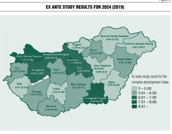
Ex ante studies show a rapid bounce back of the economy after the pandemic and a slowdown in infrastructure development (Figure 6).
The impact of the pandemic is followed by a major drop in the value of the complex development index in all counties in 2020 and 2021, followed by a slow, gradual improvement in values, but still below the 2019 level in most counties by the end of the time horizon (Table 7). The counties with the smallest deviation from 2019 levels are Győr- Moson-sopron, Baranya and Bács-Kiskun, and only the capital city shows a slight increase. The complexity of the index implies that some of its components have a delayed impact after shocks, therefore the return to the previous trajectory is slower.
SUMMARy, CoNCLUSIoNS
In addition to the analysis of economic growth, the importance of complex, holistic regional analyses, which focus on the level of development and the development path of a
given region, is growing. The events of recent years (decades) play an important role in the analysis of future development paths.
The analysis of regional development and development paths and the definition of their trends (improving, stagnating, deteriorating) is not purely self-serving, because the extent and direction of change has a significant impact on the given population’s quality of life.
In our study, we examined the past (1995- 2019) and possible future development paths of our country’s counties and Budapest between 2020 and 2024. This is a good example of how path dependency can lead to a certain powerlessness, a negative lock-in effect, from which the given region can only break
out at the cost of serious efforts and social and economic sacrifices. our model interprets regional development and development paths on the basis of a single complex, composite indicator and its changes. The indicators constituting the regional development index were selected on the basis of their statistical reliability and relevance, in a self-limiting manner.
In our analysis, an attempt was made to estimate the impact of the covid-19 epidemic (exogenous shock) on the development paths of the counties. For this purpose, we incorporated an expert panel into the model, based on which we corrected the trajectory.
our analysis confirms the following.
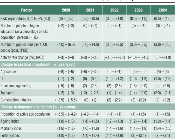
Table 6 regional inpuT assumpTions (%, year/year)
factor 2020 2021 2022 2023 2024
R&D expenditure (% of GDP), (RD) (0) – (0.5) (0.5) – (0.6) (0.5) – (1.0) (0.5) – (1.0) (0.5) – (1.0) Number of people in higher
education (as a percentage of total population, persons), (hE)
(–2) – (–3) (0) – (–1) (0) – (–1) (0) – (–1) (0) – (–1)
Number of publications per 1000 people (pcs), (PUB)
(4.0) – (6.0) (3.0) – (4.0) (3.0) – (3.5) (3.0) – (3.5) (3.0) – (3.5)
Activity rate change (%), (ACT) (–3) – (–4) (–3) – (–3.5) (–3.0) – (–3.1) (–1.0) – (–1.5) (0) – (–1.0) Change in sectoral investment (%, year/year)
Agriculture (–8) – (–6) (–6) – (–3.5) (0) – (–1) (3) – (6) (4) – (6)
IT (–1) – (–2) (0) – (0.5) (1.0) – (1.2) (1.0) – (1.2) (1.0) – (1.2)
Precision engineering (–5) – (–6) (2) – (2.5) (2) – (2.5) (1.8) – (2.0) (2) – (2.5)
Transport (–2) – (–3) (–2) – (–2.5) (1) – (1.4) (1.4) – (2.0) (2.0) – (2.1)
Construction industry (–8.5) – (–5.5) (0) – (1) (2) – (2.2) (2) – (2.2) (2) – (2.2) Change in demographic factors (%, year/year)
Proportion of active age population (–5.5) – (–4.2) (–4.9) – (–4) (–1) – (1) (1) – (1.5) (1) – (1.5) Ageing index (1.0) – (1.8) (1.4) – (1.5) (1.2) – (1.3) (1.2) – (1.4) (1.2) – (1.4) Mortality index (1.6) – (1.8) (1.6) – (1.8) (1.4) – (1.6) (1.4) – (1.6) (1.4) – (1.5) Fertility index (1.0) – (1.2) (1.1) – (1.4) (1.4) – (1.6) (2) – (2.1) (2) – (2.1) Source: own editing
Figure 6 ex anTe sTudy resulTs for 2024 (2019)
Source: own editing
Table 7 ex anTe sTudy resulTs
(forecasT of complex developmenT index: 2019, 2024)
2019 2024 change 2019 2024 change
Budapest 17.80 17.87 0.07 Tolna 4.60 4.26 –0.34
Pest 6.82 6.24 –0.58 Borsod-Abaúj-Zemplén 5.09 4.85 –0.24
Fejér 5.95 5.49 –0.46 heves 5.63 5.21 –0.42
Komárom-Esztergom 6.51 6.04 –0.47 Nógrád 4.70 4.19 –0.51
Veszprém 6.58 6.02 –0.56 hajdú-Bihar 6.40 5.83 –0.57
Győr-Moson-Sopron 7.90 7.73 –0.17 Jász-Nagykun-Szolnok 4.85 4.38 –0.47
Vas 6.34 5.87 –0.47 Szabolcs-Szatmár-Bereg 5.16 4.81 –0.35
Zala 5.71 4.97 –0.74 Bács-Kiskun 5.39 5.23 –0.16
Baranya 5.53 5.34 –0.19 Békés 4.60 4.19 –0.41
Somogy 5.43 5.01 –0.42 Csongrád-Csanád 7.15 6.69 –0.46
Source: own editing
Ex-ante study result for the complex development index
The counties have followed different development paths over the last 25 years, a trend that holds over the forecast horizon.
Development is therefore not unilinear due to the different interaction of local and regional and macro-level socio-economic factors. The development paths of counties, due to global, macro and local level traumas that occur from time to time, are more sensitive to shocks than the trajectory of specific GDP output. This effect is mostly due to the complexity of the complex index, as the shocks lead to changes in the individual indicators at different rates and to different degrees (in some cases with a significant delay). GDP per capita has been high in recent decades in regions with export- oriented sectors (mechanical engineering, automotive industry).
Economic and social history and cultural habits play an important role in the differences
in development paths. Regional resource allocations by the state reduce differences in development.
changes in the pace of development cannot be left to market processes alone, and the state still has a major role to play in the case of linear, social and environmental infrastructure interventions.
In the case of human factors (education, employment), value systems are of paramount importance. statistics show that in regions with a low level of education, this indicator has remained low in recent years, and that there will be no significant positive change in the short term.
over the last 10 years, the improvement in the quantity and quality of linear infrastructure and the increase in GDP have brought about a significant change in regional develop- ment. ■
References Note
1 see: Report of the Inter-Agency and Export Group on sustainable Development Goal Indicators, Annex III, March 2016. http://unstats.un.org/unsd/statcom/47th-session/documents/2016-2-IAEG- sDGs-E.pdf.
Ackermann, R. (2001). Pfadabhängigkeit, Institu
tionen und Regelkonform. Mohr siebeck, Tübingen Bach, st., Gorning, M., stille F., Voigt, u. (1994). Wechselwirkungen zwischen Infrastrukturausstattung, strukturellem Wandel und Wirtschaftswachstum. Duncker & Humblot, Berlin
Benedek J. (2010). Genesis and change of the Regions: chance or Necessity? Tér és Társadalom (Space and Society), 24 (3), pp. 193–201,
https://doi.org/10.17649/TET.24.3.1336
Benedek, J., Ivan, K., Török, I., Temerdek, A., Holobaca, I-H. (2020). Indicator‐based assessment of local and regional progress toward the sustainable Development Goals (sDGs): An integrated approach from Romania. Sustainable Development 2021, pp. 1–16,
https://doi.org/10.1002/sd.2180
Boschma, R. A., Lambooy, J. G. (1999).
Evolutionary economics and economic geography.
Journal of Evolutionary Economics, 9, pp. 411–429, https://doi.org/10.1007/s001910050089
camagni, R. ed. (1991). Innovation networks:
Spatial perspectives. Belhaven-Pinter, London
capello, R., Fratesi, u. (2012). Modelling Regional Growth: An Advanced MAssT Model.
Spatial Economic Analysis, 7(3), pp. 293–318, https://doi.org/10.1080/17421772.2012.694143
chizzolini, B., capello, R., camagni, R.P., Fratesi, u. (2008). Modelling Regional Scenarios for the Enlarged Europe. European Competitiveness and Global Strategies. springer-Verlag Berlin Heidelberg
clark, G. (2007). A Farewell to Alms. A Brief Economic History of the World. Princeton university Press, Princeton
crescenzi, R., Rodríguez-Pose, A. (2012).
Infrastructure and regional growth in the European union. Papers in Regional Science, 91(3), pp. 487–
513,
https://doi.org/10.1111/j.1435-5957.2012.00439.x czeczeli V., Kolozsi P. P., Kutasi G., Marton Á. (2020). Economic exposure and crisis resilience in exogenous shock. The short term economic impact of the covid-19 epidemic in the Eu. Pénzügyi Szemle (Public Finance Quarterly), 58(4), pp. 323–349, https://doi.org/10.35551/PsZ_2020_3_1
Eckey, H. F., schwengler, B., Türck, M.
(2007). Vergleich von deutschen Arbeitsmarktregionen.
IAB-Discussion Paper, 3
Faluvégi, A. (2000). Developmental differences of Hungarian micro-regions. Területi statisztika (Regional statistics), 40(4), pp. 319–346,
https://doi.org/10.15196/Ts600109
Hampel, K.E., Kunz, M., schane, N. G., Wapler, R., Weyh, A. (2007). Regional Employment Forecasts with Spatial Interdependencies, IAB Discussion Paper 02/2007
Hernandez-Murillo, R., owyang, M. T.
(2006). The information content of regional employment data forecasting aggregate conditions.
Economic Letters, (90) pp. 335–339,
https://doi.org/10.1016/j.econlet.2005.08.023 Jakab, M. Z., Világi, B. (2008). An estimated DSGE model of the Hungarian economy. MNB Working Papers (9)
Jánossy, F. (1966). Trends of economic development and recovery periods. Economic and Legal Publishing House, Budapest
Kocziszky Gy. (2008). Measurement methodology of Regional Innovation potential.
Északmagyarországi Stratégiai Füzetek (Strategic Issues of Northern Hungary), 4(2), pp. 14–34
Kocziszky, Gy., Benedek, J. (2012).
contributions to the issues of regional economic growth and equilibrium as well as the regional policy. Hungarian Geographical Bulletin, 61(2), pp.
113–130
Kocziszky, Gy., szendi, D. (2018). Regional Disparities of the social Innovation Potential in the Visegrad countries: causes and consequences.
European Journal of Social Sciences Education and Research, 12(1), pp. 35–41,
https://doi.org/10.2478/ejser-2018-0004
Kopátsy, s. (2011). New economics. The quality society. Akadémiai Kiadó, Budapest
Köppel, M. (1979). Ansatzpunkte der regionaler Wirtschaftsprognose. Eine methodenkritische untersuchung von Modellen zur Prognose der langfristigen regionalen Wirtschaftsentwicklung.
Volkswirtschaftliche Schriften, Heft 287. Duncker &
Humboldt, Berlin
Krugman, P. (1997). Development, Geography and Economic Theory. MIT Press, London