Annales Mathematicae et Informaticae (53.): Selected papers of the 1st Conference on Information Technology and Data Science

(1)

ANNALES

MATHEMATICAE ET INFORMATICAE

TOMUS 53. (2021)

COMMISSIO REDACTORIUM

Sándor Bácsó (Debrecen), Sonja Gorjanc (Zagreb), Tibor Gyimóthy (Szeged), Miklós Hoffmann (Eger), József Holovács (Eger), Tibor Juhász (Eger), László Kovács (Miskolc), Gergely Kovásznai (Eger), László Kozma (Budapest), Kálmán Liptai (Eger), Florian Luca (Mexico), Giuseppe Mastroianni (Potenza),

Ferenc Mátyás (Eger), Ákos Pintér (Debrecen), Miklós Rontó (Miskolc), László Szalay (Sopron), János Sztrik (Debrecen), Gary Walsh (Ottawa)

HUNGARIA, EGER

(2)

MATHEMATICAE ET INFORMATICAE

VOLUME 53. (2021)

EDITORIAL BOARD

Sándor Bácsó (Debrecen), Sonja Gorjanc (Zagreb), Tibor Gyimóthy (Szeged), Miklós Hoffmann (Eger), József Holovács (Eger), Tibor Juhász (Eger), László Kovács (Miskolc), Gergely Kovásznai (Eger), László Kozma (Budapest), Kálmán Liptai (Eger), Florian Luca (Mexico), Giuseppe Mastroianni (Potenza),

Ferenc Mátyás (Eger), Ákos Pintér (Debrecen), Miklós Rontó (Miskolc), László Szalay (Sopron), János Sztrik (Debrecen), Gary Walsh (Ottawa)

INSTITUTE OF MATHEMATICS AND INFORMATICS ESZTERHÁZY KÁROLY UNIVERSITY

HUNGARY, EGER

(3)

(4)

1 ^st Conference on Information Technology

and Data Science

The conference was organized by

Faculty of Informatics, University of Debrecen, Hungary, November 6–8, 2020

Conference Chairmen István Fazekas and András Hajdu

The conference was supported by the construction EFOP-3.6.3-VEKOP-16-2017-00002.

The project was co-financed by the

Hungarian Government and the European Social Fund.

(5)

A kiadásért felelős az Eszterházy Károly Egyetem rektora Megjelent a Líceum Kiadó gondozásában

Kiadóvezető: Dr. Nagy Andor Felelős szerkesztő: Dr. Domonkosi Ágnes

Műszaki szerkesztő: Dr. Tómács Tibor Megjelent: 2021. május

(6)

Enhanced optimization of high order concentrated matrix-exponential

distributions ^∗

Salah Al-Deen Almousa

^a

, Miklós Telek

^ab

aDepartment of Networked Systems and Services Technical University of Budapest

Budapest, Hungary

bMTA-BME Information Systems Research Group Budapest, Hungary

almousa@hit.bme.hu telek@hit.bme.hu Submitted: November 23, 2020

Accepted: February 11, 2021 Published online: May 18, 2021

Abstract

This paper presents numerical methods for finding high order concentrated matrix-exponential (ME) distributions, whose squared coefficient of variation (SCV) is very low. Due to the absence of symbolic construction to obtain the most concentrated ME distributions, non-linear optimization problems are defined to obtain high order concentrated matrix-exponential (CME) distributions . The number of parameters to optimize increases with the order in the “full” version of the optimization problem. For orders, where

“full” optimization is infeasible (𝑛 >184), a “heuristic” optimization procedure, optimizing only 3 parameters independent of the order, was proposed in [6].

In this work we present an enhanced version of this heuristic optimization procedure, optimizing only 6 parameters independent of the order, which results in CME distributions with lowerSCVthan the existing 3-parameter method. TheSCV gain of the new procedure compared to the old one is

∗This work is partially supported by the OTKA K-123914 and the NKFIH BME NC TKP2020 projects.

doi: https://doi.org/10.33039/ami.2021.02.001 url: https://ami.uni-eszterhazy.hu

5

(7)

approximately1.66 and it is almost independent of the order. The range of the applicability of the heuristic optimization methods extends to order 𝑛= 5000.

To further extend the range of available CME distributions, we also propose a parameter extrapolation approach, which provides CME distributions until order𝑛= 20000. TheSCVof the obtained order20000CME distribution is≈10⁻⁹.

Keywords:Squared coefficient of variation, optimization, concentrated matrix exponential distributions, extrapolation

AMS Subject Classification:65K10, 90C31

1. Introduction

Highly concentrated matrix-exponential functions are useful in many research areas, for example, in numerical inverse Laplace transform (NILT) methods [5], as well in numerical inverse Z-transform (NIZT) methods [7]. Recently, Akar et al.

[1], proposed the ME-fication technique, in which a concentrated matrix exponenti- ation distribution replaces the Erlang distribution for approximating deterministic time horizons.

Concentrated ME distributions of order𝑁, with𝑁 = 2𝑛+ 1,¹ are abbreviated as CME(𝑁). CME distributions successfully constructed in [6] in the range of𝑁 = 369, . . . ,2001are based on a heuristic numerical optimization procedure optimizing 3 parameters independent of the order. This preliminary result indicated that the minimal SCV of CME(𝑁) is less than 1/𝑁². The reasons for applying a heuristic approach are that there is no symbolic construction available to obtain the most concentrated ME distribution, and the full numerical optimization-based approaches (i.e., where the number of parameters to optimize is increasing with 𝑁) get to be prohibitively complex for 𝑁 > 369 according to [6]. In this work we aim at improving the heuristic optimization procedure presented in [6], which we refer to as 3-parameter optimization. The proposed enhanced optimization procedure optimizes 6 parameters (independent of the order) and we will refer to it as 6-parameter optimization method.

The rest of the paper is organized as follows. In Section 2 we provide a brief introduction of ME distributions and discuss the definition of SCV and the optimization problem to obtain its minimum. In Section 3 we review the optimization methods proposed for SCVminimization in the literature and discuss their applicability. Section 4 introduces the proposed enhancedSCVoptimization procedure with 6 parameters and Section 5 discusses its numerical properties. Section 6 presents the parameter extrapolation approach to extend the availability of CME distributions up to order𝑛= 20000. Finally, Section 7 concludes the paper.

1Both of these two order definitions are present in the related literature.𝑁, “the cardinality of the describing matrix”, is more commonly used in phase type and matrix exponential distribution related literature, while𝑛, “the number of complex conjugate eigenvalue pairs” is more commonly used in NILT related literature.

(8)

2. Matrix exponential distributions

Definition 2.1. Order𝑁 ME functions(referred to as ME(𝑁)) are given by

𝑓(𝑡) =𝛼𝑒^A𝑡(−A)1, (2.1)

where 𝛼is a real row vector of size𝑁,A is a real matrix of size𝑁×𝑁 and 1is the column vector of ones of size𝑁.

Definition 2.2. If 𝑓(𝑡) ≥0,∀𝑡 ≥ 0, and 𝛼 is such that 𝛼1 = 1then 𝑓(𝑡) is the probability density function of aME distribution of order𝑁.

According to (2.1), vector𝛼and matrixAdefine a matrix exponential function.

We refer to the pair(𝛼,A)as matrix representation in the sequel.

An ME distribution is said to be concentrated when its squared coefficient of variation

𝑆𝐶𝑉(𝑓(𝑡)) = 𝜇0𝜇2

𝜇²₁ −1, (2.2)

is low. In (2.2), 𝜇𝑖 denotes the 𝑖th moment, defined by 𝜇𝑖 = ∫︀∞

𝑡=0𝑡^𝑖𝑓(𝑡)𝑑𝑡. We note that the SCV according to (2.2) is insensitive to multiplication and scaling, i.e. 𝑆𝐶𝑉(𝑓(𝑡)) =𝑆𝐶𝑉(𝑐𝑓(𝜆𝑡)).

The optimization problem to obtain the minimalSCV of ME(𝑁) can be for- mulated as

min𝛼,A𝑆𝐶𝑉(𝑓(𝑡)) subject to𝑓(𝑡)≥0, ∀𝑡 >0.

Although matrix-exponential functions have been used for many decades, there are still many questions open regarding their properties. Such an important ques- tion is how to decide efficiently if a matrix-exponential function is non-negative for ∀𝑡 >0. In general, 𝑓(𝑡)≥0,∀𝑡 >0 does not necessarily hold for given (𝛼,A) representation, and it is rather difficult to check. A potential numerical solution for checking this property is proposed in [9].

Due to the difficulty of checking the constraints of the above constrained optimization problem, its solution is an open problem currently.

3. Concentrated ME distributions

A possible way to simplify the constrained optimization problem is to search for the minimum in a special subset of ME(𝑁), which is non-negative by construction.

Horváth et al. in [6] suggest such a subset which is characterized by

𝑓(𝑡) =𝑐𝑓⁺(𝜆𝑡), (3.1)

(9)

where𝑓⁺(𝑡)is an exponential cosine-square function with order𝑛defined as 𝑓⁺(𝑡) =𝑒^−𝑡

∏︁𝑛 𝑗=1

cos²

(︂𝜔𝑡−𝜑𝑗

2 )︂

, (3.2)

where𝜔≥0 and0≤𝜑𝑗 <2𝜋for𝑗∈ {1, . . . , 𝑛}.

In [6] the authors conjectured that the density function of the most concentrated ME distribution of order𝑁 belongs to this special class of ME(𝑁), but the validity of this conjecture is not proved even for the smallest non-obvious case,𝑁 = 3.

An exponential cosine-square function is a non-negative (due to its construction) matrix exponential function and [8, Appendix A] presents how to obtain the matrix representation of size𝑁 = 2𝑛+ 1associated with𝑓⁺(𝑡)in (3.2). Consequently, the set of exponential cosine-square functions of order 𝑛is a special subset of ME(𝑁) (where𝑁 = 2𝑛+ 1).

In this paper, we make use the fact that exponential cosine-square functions can also be represented in the following hyper-exponential form [6]

𝑓⁺(𝑡) =𝑒^−𝑡

∏︁𝑛 𝑗=1

cos²

(︂𝜔𝑡−𝜑𝑗

2 )︂

=

∑︁2𝑛 𝑘=0

𝜂𝑘𝑒^−𝛽^𝑘^𝑡, 𝑡≥0, (3.3) where the 𝜂𝑘, 𝛽𝑘 (𝑘 = 0, . . . ,2𝑛) coefficients contain complex conjugate pairs.

Generally, calculating the 𝜇0, 𝜇1, 𝜇2 moments based on (3.2), is not an easy task due to computational complexity caused by the product of the cosine square terms.

Instead calculating the𝜇0, 𝜇1, 𝜇2 moments based on (3.3) is much easier since

𝜇𝑖=

∫︁∞ 𝑡=0

𝑡^𝑖

∑︁2𝑛 𝑘=0

𝜂𝑘𝑒⁻^𝛽^𝑘^𝑡𝑑𝑡=

∑︁2𝑛 𝑘=0

𝑖!𝜂𝑘

𝛽_𝑘^𝑖+1, (3.4)

3.1. Full optimization of the 𝑓

⁺

(𝑡) parameters

In the sequel, we utilize the fact that multiplication and scaling (with 𝑐 and 𝜆 in (3.1)) does not effect the SCV and optimize the SCV of𝑓⁺(𝑡) instead of𝑓(𝑡).

𝑓⁺(𝑡)in (3.2) is defined by𝑛+ 1parameters: the frequency𝜔 and the zeros𝜑𝑗 for 𝑗= 1, . . . , 𝑛.Unfortunately,𝑆𝐶𝑉(𝑓⁺(𝑡))is not a simple function of the parameters.

For a given 𝑛to find𝑓⁺(𝑡)with minimalSCV, i.e.

𝜔,𝜑min1,...,𝜑𝑛

𝑆𝐶𝑉(𝑓⁺(𝑡))

is still a hard non-linear optimization problem, where the number of parameters to optimize is𝑛+ 1.

Numerical methods for the solution of this problem are discussed in [6]. The main findings reported there are that evolution strategy based optimization provided the best numerical results. The solution of the problem with theCMA-ES

(10)

method [4] is fast, but does not find the best optimum compared to the BIPOP- CMA-ES method [3], which is much slower. The applicability of the two methods are 𝑛 ≤ 74 (𝑁 ≤ 149) in case of the BIPOP-CMA-ES method and 𝑛 ≤ 184 (𝑁 ≤ 369) in case of the CMA-ES method. For these orders the respective the optimization procedures take several days to terminate on an average PC. The computational complexity of these procedures increases super linearly with the order 𝑛, which inhibits the application of these procedure for higher orders.

3.2. Heuristic optimization of the 𝑓

⁺

(𝑡) parameters

To go beyond order 𝑛 = 184, [6] proposed a sub-optimal, 3-parameter heuristic optimization procedure, that reduce the complexity of the optimization problem by reducing the number of parameters to optimize to three, independent of the order.

Figure 2 displays the location of the the 𝜑𝑗 parameters obtained by the full optimization method for 𝑛 = 74. As it is visible in the figure, there is a gap between the 𝜑𝑗 parameters at around 𝑝≈ 5.2 and the size of that gap, which is the maximum value in Figure 1 is around 𝑤 ≈0.28. The heuristic optimization procedure proposed in [6] assumes that the 𝜑𝑗 parameters are equidistant below and above that gap. Figure 1 and 2 display how good this assumption is compared to the fully optimized𝜑𝑗 parameters.

Since the 𝜑𝑗 parameters are located between 0 and 2𝜋 and the number of parameters are𝑛, this assumption allows to determine the𝜑𝑗 parameters based on 𝑝and𝑤according to the following expression

𝜑𝑗=

{︂ (𝑗−1/2)𝑑 if𝑗≤𝑖,

(𝑗−1/2)𝑑+𝑤 if𝑗 > 𝑖. (3.5) where

𝑑=2𝜋−𝑤 𝑛 , 𝑖=

⌊︂𝑝−𝑤/2

𝑑 +1

2

⌋︂

. (3.6)

With the use of (3.5),𝑓⁺(𝑡)is defined by the parameters 𝜔,𝑝and 𝑤and the related optimization problem is

min𝜔,𝑝,𝑤𝑆𝐶𝑉(𝑓⁺(𝑡)),

subject to: 0< 𝑝−𝑤/2< 𝑝+𝑤/2<2𝜋, 𝜔 >0.

The solution of this optimization problem is computed by the CMA-ES method up to 𝑛 = 1000 in [6]. Moreover, in this work we expand this solution up to 𝑛= 5000.

(11)

4. Enhanced heuristic optimization of 𝑆𝐶𝑉 (𝑓

⁺

(𝑡)) with 6 parameters

Figure 1 and 2 suggests that the equidistant location of the𝜑𝑗parameters according to (3.5) is not flexible enough to obtain similar low SCV as obtained with the full optimization method. Starting from this assumption, we try to locate the𝜑𝑗

parameters in a more flexible way. To this end we introduce two different power functions below and above the gap of the𝜑𝑗 parameters as follows

𝜑𝑗(𝑎1, 𝑏1, 𝑎2, 𝑏2, 𝑖, 𝛾, 𝛿) =

{︂ 𝑎1+𝑏1𝑗^𝛾 for1≤𝑗 ≤𝑖,

𝑎2+𝑏2𝑗^𝛿 for𝑖+ 1≤𝑗≤𝑛. (4.1) The auxiliary parameters, 𝑎1, 𝑏1, 𝑎2, 𝑏2, can be transformed to a set of more expressive parameters based on the following relations

𝜑1= 0, 𝜑𝑖=𝑝−𝑤/2, 𝜑𝑖+1=𝑝+𝑤/2, 𝜑𝑛+1= 2𝜋. (4.2) Substituting these relations into (4.1) results in the following function for the 𝜑𝑗

parameters

𝜑𝑗(𝑝, 𝑤, 𝑖, 𝛾, 𝛿) =

⎧⎨

⎩

(𝑝−𝑤/2)𝑗^𝛾

(𝑖^𝛾−1) −^𝑝(𝑖⁻^𝛾^𝑤/2−1) for1≤𝑗≤𝑖, 2𝜋−(^𝑗^𝛿−(𝑛+1)^𝛿)(2𝜋−𝑝−𝑤/2)

((𝑖+1)^𝛿−(𝑛+1)^𝛿) for𝑖+ 1≤𝑗≤𝑛. (4.3) In (4.3) the parameters are constrained by

0< 𝑝−𝑤/2< 𝑝+𝑤/2<2𝜋, 𝛾 >0, 𝛿 >0.

The intuitive meaning of the parameters in (4.3) are as follows: the meaning of 𝑝,𝑤,𝜔, and𝑖are the same as in the 3-parameter optimization method, i.e.

• 𝑖: is the number of𝜑𝑗 parameters left to the gap,

• 𝑝,𝑤: are the midpoint of the gap and its width,

while𝛾and𝛿are shape parameters defining the power series of the𝜑𝑗 parameters below and above the gap.

Based on (4.3), which defines the 𝜑𝑗 parameters based on 5 parameters, the optimization of𝑆𝐶𝑉(𝑓⁺(𝑡))for a given order𝑛is the following 6-parameter optimization problem

min𝜔,𝑝,𝑤,𝑖,𝛾,𝛿𝑆𝐶𝑉(𝑓⁺(𝑡))

subject to: 0< 𝑝−𝑤/2< 𝑝+𝑤/2<2𝜋, 𝛾 >0, 𝛿 >0, 𝜔 >0,

where𝑝, 𝑤, 𝑖, 𝛾, 𝛿define the𝜑𝑗parameters according to (4.3) and the𝜑𝑗parameters and𝜔 define𝑓⁺(𝑡)according to (3.2).

To solve this optimization problem we propose to compute theSCVaccording to Algorithm 1 and obtain the optimum by the CMA-ES method using Algorithm

(12)

1 as the objective function. The procedure to obtain𝜂𝑖,𝛽𝑖 and the required high precision arithmetic are detailed in [6]. Here we only recall that all computations can be performed with standard double precision arithmetic except the ones indicated to be “high precision”. In those cases, to obtain results in16digits precision, the required numerical precision is0.647𝑛+ 17.478 digits for ME(2𝑛+ 1).

Algorithm 1 The objective function of the heuristic method.

1: procedureComputeSCV(𝜔, 𝑝, 𝑤, 𝑖, 𝛾, 𝛿)

2: Obtain𝜑𝑗 for𝑗∈ {1, . . . , 𝑛} by (4.3)

3: Compute𝜂𝑖,𝛽𝑖 (high precision) by (3.3)

4: Compute𝜇𝑖 (high precision) by (3.4)

5: Compute𝑆𝐶𝑉 by (2.2)

6: return𝑆𝐶𝑉

7: end procedure

5. Numerical properties

The behaviour of the𝜑𝑗 parameters obtained by the proposed 6-parameter heuristic method is also depicted in Figure 1 and 2. The figures suggest, that the 𝜑𝑗

parameters obtained by the 6-parameter optimization method better approximate the behaviour of the𝜑𝑗 parameters obtained by full optimization than the ones of the 3-parameter method.

10 20 30 40 50 60 73

0 0.1 0.2 0.3 0.4

𝑗 𝜑𝑗+1−𝜑𝑗

BIPOP-CMA-ES 3-parameter heuristic 6-parameter heuristic

Figure 1. Difference of consecutive𝜑𝑗values obtained by full optimization, 3-parameter optimization and the proposed 6-parameter

optimization for order𝑛= 74.

Moreover, Figure 2 displays how the distribution of𝜑𝑗 locations are influenced

(13)

by the shaping parameters 𝛾, 𝛿, and getting closer (compared to the 3-parameter case) to the fully optimized ones. This improvement in the positioning of the 𝜑𝑗 parameters leads to a significant SCV reduction compared to the 3-parameter method as illustrated in Figure 3.

10 20 74

0 2 4 6

𝑗 𝜑𝑗

BIPOP-CMA-ES 3-parameter heuristic 6-parameter heuristic

Figure 2. The location of the𝜑𝑗parameters obtained by full optimization, 3-parameter optimization and the proposed 6-parameter

optimization for order𝑛= 74.

74 200 500 1000 5000

0.00000001 0.0000001 0.000001 0.00001 0.0001

𝑛= (𝑁 −1)/2

𝑆𝐶𝑉𝑛

6-parameter heuristic 3-parameter heuristic

CMA-ES

Figure 3. The minimal SCV values obtained by full optimization, 3-parameter optimization and the proposed 6-parameter optimiza-

tion as a function of order𝑛in log-log scale.

In the depicted range the gain (the ratio of the SCV obtained by the two

(14)

methods) is approximately 1.66 and it is almost independent of the order. The proposed heuristic optimization resulted in almost the same SCV values as the ones obtained by the full optimization method in the range where full optimization is feasible and beyond that order (𝑛 >184) the 6-parameter optimization results seem to follow the same decay trend.

We believe with some confidence in the possibility of expanding the heuristic optimization for orders larger than 𝑛 = 5000, using a more powerful computing device.

Figure 4 depicts the running time of the heuristic optimization procedure on an average PC clocked at 2.9 GHz as a function of the order𝑛.

180 1000 2000 5000

1 10 100 1000 10000

𝑛

Timeinminutes

6-parameter heuristic 3-parameter heuristic

Figure 4. Running time of the heuristic parameter optimization procedures for different orders in log-log scale.

6. Extrapolation of the parameters of heuristic op- timization

The high computational costs of the heuristic optimization methods, plotted in Figure 4, inhibits their application for orders higher than 𝑛= 5000. In this section, we intend to obtain CME distributions for orders𝑛 >5000by extrapolating parameters of the heuristic optimization procedures.

Letv(𝑛)denote the parameter values obtained from the heuristic optimization method for order𝑛, that is, for the 3-parameter methodv(𝑛) ={𝜔(𝑛), 𝑝(𝑛), 𝑤(𝑛)} and for the 6-parameter method v(𝑛) = {𝜔(𝑛), 𝑝(𝑛), 𝑤(𝑛), 𝑖(𝑛), 𝛾(𝑛), 𝛿(𝑛)}. Fur- ther more, let𝒩 ={𝑛1, 𝑛2, . . . , 𝑛𝐾}be the set of𝐾orders for which the parameter is available (the heuristic optimization is performed) 𝑛𝐾 = 5000 in our case and the other evaluated orders are visible in Figure 4.

(15)

6.1. Extrapolation methods

To extrapolate the v(𝑛)vector for𝑛 >5000we considered the following extrapolation approaches.

• Element-wise extrapolation ofv(𝑛)

In this set of methods the elements ofv(𝑛)are extrapolated independent of each others.

– Polynomial extrapolation (𝑘+ 1parameters):

ˆ

𝑣𝑖(𝑛) =𝑎𝑖+𝑏𝑖𝑛+𝑐𝑖𝑛²+. . .+𝑧𝑖𝑛^𝑘, (6.1) where 𝑣𝑖(𝑛) is the 𝑖th element of v(𝑛) and 𝑖 ∈ {1,2,3} in case of the 3-parameter method and 𝑖 ∈ {1,2, . . . ,6} in case of the 6-parameter method.

– Power function extrapolation (3parameters):

ˆ

𝑣𝑖(𝑛) =𝑎𝑖𝑛^𝑏^𝑖+𝑐𝑖. (6.2) – Exponential extrapolation (3 parameters):

ˆ

𝑣𝑖(𝑛) =𝑎𝑖𝑒^𝑏^𝑖^𝑛+𝑐𝑖. (6.3) In the element-wise extrapolation, we apply the following distance measure forˆ𝑣𝑖(𝑛)

𝒟^𝑖= 1 𝐾

∑︁

𝑛∈𝒩

|𝑣𝑖(𝑛)−𝑣ˆ𝑖(𝑛)|. (6.4) That is, in power function and exponential extrapolation, the optimal extrapolation parameters are obtained as

{𝑎^*_𝑖, 𝑏^*_𝑖, 𝑐^*_𝑖}= arg min_{_𝑎_𝑖_,𝑏_𝑖_,𝑐_𝑖_}𝒟^𝑖, (6.5) and in polynomial extrapolation, the{𝑎𝑖, 𝑏𝑖, . . . , 𝑧𝑖}parameters are obtained similarly.

• Vector-wise extrapolation ofv(𝑛)

– Vector polynomial extrapolation ((𝑚+𝑘)𝑚parameters):

^ v(𝑛) =(︀

a+b𝑛+c𝑛²+. . .+z𝑛^𝑘)︀

G, (6.6)

where each row sum ofGis one (and this wayGcontains(𝑚−1)𝑚free parameters),𝑚 is the number of elements of v. 𝑚= 3or 6 depending on the applied heuristic optimization.

(16)

– Matrix power function extrapolation ((𝑚+ 2)𝑚parameters):

ˆ

v(𝑛) =aDiag⟨𝑛^𝑏¹, . . . , 𝑛^𝑏^𝑚⟩G+c. (6.7) – Matrix exponential extrapolation ((𝑚+ 2)𝑚parameters):

ˆ

v(𝑛) =aDiag⟨𝑒^𝑏¹^𝑛, . . . , 𝑒^𝑏^𝑚^𝑛⟩G+c. (6.8) In case of vector-wise extrapolation we apply the 𝐿² vector norm as the distance measure

𝒟= 1 𝐾

∑︁

𝑛∈𝒩

||v(𝑛)−v(𝑛)ˆ ||²= 1 𝐾

∑︁

𝑛∈𝒩

⎯⎸

⎸⎷

∑︁𝑚 𝑖=1

(v𝑖(𝑛)−vˆ𝑖(𝑛))². (6.9) That is, in Matrix power and Matrix exponential extrapolation, the optimal parameters are obtained as

{a^*,b^*,c^*,G^*}= arg min_{_a,b,c,G_}𝒟 (6.10) and the Matrix polynomial case is optimized similarly according to its parameters.

We note that the results obtained by any of these methods are sensitive for𝒩, the set of orders which are considered in the parameter estimations. That is, different extrapolation parameters are obtained by the same extrapolation procedure for different 𝒩 sets. Generally, we used the optimization results between orders 400 and5000, that is,400≤𝑛≤5000for∀𝑛∈ 𝒩.

The goodness of an extrapolation approach can be judged by computing the SCVobtained from the extrapolated parameters and checking if the trend of decay for the given order𝑛 >5000follows the trend obtained by the heuristic method for order𝑛≤5000and plotted in Figure 3. Based on this goodness measure, we found all extrapolation approaches inappropriate except the element-wise power function extrapolation for all parameters, whose results are presented in the following subsection.

6.2. Element-wise power function extrapolation

Below, we present the results of the element-wise power function extrapolation method which we obtained by the CF tool of Matlab Curve Fitting Toolbox [2].

6.2.1. Extrapolation for the 3-parameter heuristic method

As discussed in [6] and in subsection 3.2, the 3-parameter heuristic optimization procedure minimizes the SCV as a function of 𝜔, 𝑝, 𝑤. The procedure can be applied with reasonable computation time (c.f. Figure 4) up to order 𝑛 = 5000.

Beyond this limit we apply the element-wise power function extrapolation according to (6.2), (6.4), and (6.5).

(17)

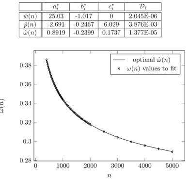
Table 1. The optimal extrapolation parameters for𝜔,𝑝and𝑤.

𝑎^*_𝑖 𝑏^*_𝑖 𝑐^*_𝑖 𝒟𝑖

ˆ

𝑤(𝑛) 25.03 -1.017 0 2.045E-06 ˆ

𝑝(𝑛) -2.691 -0.2467 6.029 3.876E-03 ˆ

𝜔(𝑛) 0.8919 -0.2399 0.1737 1.377E-05

0 1000 2000 3000 4000 5000

0.28 0.3 0.32 0.34 0.36 0.38

𝑛

𝜔(𝑛)

optimal𝜔(𝑛)^ 𝜔(𝑛)values to fit

Figure 5. Curve fitting for𝜔(𝑛)using a power function according to (6.2).

Table 1 summarizes the results for all the three parameters and Figure 5 demon- strate the quality of the obtained result for the𝜔 parameter.

Based on the extrapolation parameters in Table 1 and the associated extrapolation model in (6.2) we can extrapolate the 𝜔(𝑛), 𝑝(𝑛), 𝑤(𝑛) for orders larger than 5000. Using those extrapolated 𝜔(𝑛),ˆ 𝑝(𝑛),ˆ 𝑤(𝑛)ˆ values, Figure 6 and Ta- ble 2 present the associated SCV as a function of the order up to 𝑛 = 20000.

Figure 6 and Table 2 indicate that the SCV values obtained by the extrapolation method follow the same decay trend of the heuristic optimization. For orders less than 5000, Table 2 also compares the𝜔(𝑛), 𝑝(𝑛), 𝑤(𝑛)values obtained from the 3-parameter heuristic method, and the 𝜔(𝑛),ˆ 𝑝(𝑛),ˆ 𝑤(𝑛)ˆ values provided by the power function extrapolation method. For those orders theSCV value computed by the𝜔(𝑛), 𝑝(𝑛), 𝑤(𝑛)and the𝜔(𝑛),ˆ 𝑝(𝑛),ˆ 𝑤(𝑛)ˆ parameters are identical in their first 3 digits.

Based on Figure 6 and Table 2 we conclude that the extrapolation of the ˆ

𝜔(𝑛), 𝑝(𝑛),ˆ 𝑤(𝑛)ˆ parameters with the element-wise power function extrapolation provide fairly concentrated matrix exponential distributions up to order 20000, whoseSCV follows the same decay trend for as the one of the 3-parameter heuristic method up to order5000.

(18)

74 200 1000 5000 20000 0.000000001

0.00000001 0.0000001 0.000001 0.00001 0.0001

𝑛= (𝑁−1)/2 𝑆𝐶𝑉𝑛

CMA-ES 6-parameter heuristic 3-parameter heuristic 6-parameter extrapolate 3-parameter extrapolate

Figure 6. The approximated and the heuristics SCV as a function of order𝑛in log-log scale.

Table 2. Original and extrapolated parameters and the associated SCVfor the 3-parameter heuristic optimization.

Heuristic Optimization Extrapolation

𝑛 𝑤(𝑛) 𝑝(𝑛) 𝜔(𝑛) SCV 𝑤(𝑛)ˆ 𝑝(𝑛)ˆ 𝜔(𝑛)ˆ SCV

400 0.0563612 5.4162 0.385725 3.5945E-06 0.0565153 5.41526 0.3855761 3.5947992E-06 800 0.0278559 5.51193 0.353088 8.53737E-07 0.0279266 5.51173 0.3531175 8.538201E-07 1200 .0184659 5.56361 0.336537 3.69091E-07 0.0184899 5.56096 0.3364873 3.691452E-07 1500 0.014703 5.58534 0.328039 2.32831E-07 0.014735 5.58603 0.328002 2.32849E-07 2000 0.0109708 5.61548 0.317745 1.28656E-07 0.010997 5.61638 0.317712 1.28668E-07 2500 0.00874565 5.63895 0.310221 8.12596E-08 0.008765 5.63848 0.310205 8.12665E-08 3000 0.0072661 5.65621 0.304338 5.58463E-08 0.007281 5.65565 0.304363 5.58511E-08 3500 0.00621258 5.66986 0.299541 4.06814E-08 0.006225 5.66958 0.299619 4.06848E-08 4000 0.00542217 5.68131 0.295500 3.09232E-08 0.005434 5.68123 0.295650 3.09269E-08 4500 0.0048099 5.69091 0.292034 2.42819E-08 0.004821 5.69119 0.292252 2.42852E-08 5000 0.00432189 5.69975 0.289008 1.95615E-08 0.004331 5.69986 0.289293 1.9564E-08

10000 - - - - 0.002140 5.75159 0.271585 4.73132E-09

15000 - - - - 0.001417 5.77800 0.262512 2.06641E-09

20000 - - - - 0.001057 5.79519 0.256589 1.14904E-09

6.2.2. Extrapolation for the 6-parameter heuristic method

We applied the same extrapolation approach for the parameters of the 6-parameter heuristic method using the element-wise power function approximation according to (6.2), (6.4), and (6.5). The obtained optimal extrapolation parameter values are summarized in Table 3. Using the associated 𝑤(𝑛),ˆ 𝑝(𝑛),ˆ 𝜔(𝑛),ˆ ˆ𝑖(𝑛), ˆ𝛾(𝑛), ˆ𝛿(𝑛) functions, we also computed the SCV up to order 15000. The results are plotted in Figure 6. Unfortunately, the SCV values obtained by this 6-parameter

(19)

extrapolation methods do not follow the same decay as the one of the 6-parameter heuristic method up to𝑛= 5000. At around, 𝑛= 15000 theSCV obtained from the 6-parameter extrapolation gets to be as high as the one obtained from the 3-parameter extrapolation. Most probable, the reason for this behaviour is the instability caused by the higher number of extrapolated parameters.

Table 3. Optimal extrapolation parameters based on the 6-parameter heuristic optimization method according to (6.2).

𝑎^*_𝑖 𝑏^*_𝑖 𝑐^*_𝑖 𝒟𝑖

ˆ

𝑤(𝑛) 21.59 -1.017 0 1.958E-03 ˆ

𝑝(𝑛) -26.35 -0.9762 5.653 1.963E-02 ˆ

𝜔(𝑛) 0.8952 -0.2458 0.1318 4.484E-03 ˆ𝑖(𝑛) 0.9001 1 -0.7137 1.569 ˆ

𝛾(𝑛) 3.631 -0.76579 0.9988 3.98E-03 ˆ𝛿(𝑛) 10.48 -0.4475 0.8504 1.393E-01

Figure 7 plots the time to compute theSCV as a function of the order on a regular PC. The computation time is practically identical for both methods because the most expensive step of the computation is to transform the cosine-square form into the hyper-exponential form according to (3.3), which is need in both cases.

5000 10000 15000 20000

10 100 1000

𝑛

Timeinminutes

6-parameter extrapolation 3-parameter extrapolation

Figure 7. Running time of the parameter approximation procedures for different orders in log-log scale.

Our full C++ implementation for the 3 and 6-parameter heuristic optimization methods is reachable atwebspn.hit.bme.hu/~almousa/tools/CME_heur_approx.

zip. The procedure uses extended floating point arithmetic when needed and it also contain the CMA-ES method, which is the optimization engine applied in the 3 and 6-parameter heuristic optimization methods

(20)

7. Conclusion

We propose an efficient 6-parameter heuristicSCVoptimization procedure for concentrated matrix exponential distributions. The SCV values resulted by this 6- parameter optimization procedure are rather close to the ones obtained by the full optimization methods when both methods are feasible to compute, and seem to follow the sameSCVdecay trend for larger orders. Due to the exponential increase of the computation time as a function of the order, the applicability of the proposed heuristic optimization method extends to order 𝑛= 5000.

For larger orders, we also propose a parameter extrapolation approach which allowed us to obtain CME distributions up to order20000, such that the decay of the SCV follows the same trend as the one of the optimization procedures up to order5000.

References

[1] N. Akar,O. Gursoy,G. Horvath,M. Telek:Transient and First Passage Time Dis- tributions of First-and Second-order Multi-regime Markov Fluid Queues via ME-fication, Methodology and Computing in Applied Probability (2020), pp. 1–27,

doi:https://doi.org/10.1007/s11009-020-09812-y.

[2] Curve Fitting Toolbox, https : / / www . mathworks . com / help / curvefit, MATLAB: User’s Guide. MathWorks, 2001.

[3] N. Hansen:Benchmarking a BI-population CMA-ES on the BBOB-2009 function testbed, in: Proceedings of the 11th Annual Conference Companion on Genetic and Evolutionary Computation Conference: Late Breaking Papers, ACM, 2009, pp. 2389–2396,

doi:https://doi.org/10.1145/1570256.1570333.

[4] N. Hansen:The CMA evolution strategy: a comparing review, in: Towards a New Evolution- ary Computation, Springer, 2006, pp. 75–102,

doi:https://doi.org/10.1007/3-540-32494-1_4.

[5] G. Horváth,I. Horváth,S. A.-D. Almousa,M. Telek:Numerical inverse Laplace transformation using concentrated matrix exponential distributions, Performance Evaluation 137 (2020), p. 102067,

doi:https://doi.org/10.1016/j.peva.2019.102067.

[6] G. Horváth,I. Horváth,M. Telek:High order concentrated matrix-exponential distributions, Stochastic Models 36.2 (2020), pp. 176–192,

doi:https://doi.org/10.1080/15326349.2019.1702058.

[7] I. Horváth,A. Mészáros,M. Telek:Numerical Inverse Transformation Methods for Z- Transform, Mathematics 8.4 (2020), p. 556,

doi:https://doi.org/10.3390/math8040556.

[8] I. Horváth,O. Sáfár,M. Telek,B. Zámbó:Concentrated matrix exponential distributions, in: European Workshop on Performance Engineering, Springer, 2016, pp. 18–31,

doi:https://doi.org/10.1007/978-3-319-46433-6_2.

[9] P. Reinecke,M. Telek:Does a given vector-matrix pair correspond to a PH distribution, Performance Evaluation 80.0 (2014), pp. 40–51,

doi:https://doi.org/10.1016/j.peva.2014.08.001.

(21)

(22)

Markov modeling of traffic flow in Smart Cities ^∗

Norbert Bátfai, Renátó Besenczi, Péter Jeszenszky, Máté Szabó, Márton Ispány

Faculty of Informatics, University of Debrecen, Hungary besenczi.renato@inf.unideb.hu

jeszenszky.peter@inf.unideb.hu szabo.mate@inf.unideb.hu ispany.marton@inf.unideb.hu

Submitted: January 15, 2021 Accepted: April 25, 2021 Published online: May 18, 2021

Dedicated to the kind memory of our colleague, Norbert Bátfai.

Abstract

Modeling and simulating the traffic flow in large urban road networks are important tasks. A mathematically rigorous stochastic model proposed in [8]

is based on the synthesis of the graph and Markov chain theories. In this model, the transition probability matrix describes the traffic dynamics and its unique stationary distribution approximates the proportion of the vehicles at the segments of the road network. In this paper various Markov models are studied and a simulation method is presented for generating random traffic trajectories on a road network based on the two-dimensional stationary distribution of the models. In a case study we apply our method to the central region of the city of Debrecen by using the road network data from the OpenStreetMap project which is available publicly.

∗Renátó Besenczi and Márton Ispány are supported by Project no. TKP2020-NKA-04 which has been implemented with the support provided from the National Research, Development and Innovation Fund of Hungary, financed under the 2020-4.1.1-TKP2020 funding scheme. Péter Jeszenszky and Máté Szabó are supported by the EFOP-3.6.1-16-2016-00022 project. The project is co-financed by the European Union and the European Social Fund.

doi: https://doi.org/10.33039/ami.2021.04.008 url: https://ami.uni-eszterhazy.hu

21

(23)

Keywords:Road network, traffic simulation, discrete time Markov chain, stationary distribution, OpenStreetMap

1. Introduction

Recently, the research and development of Smart City applications have become more important by providing services to inhabitants which can make everyday life easier [15]. These applications are based on emerging technologies such as big data analytics, cloud computing, and complex sensor systems (IoT) that can support their operation. By the year 2050, 70% of Earth’s population is expected to live in cities [5] whose infrastructures will face new challenges, e.g., in the field of urban traffic. In the past few years, many developments have occurred in the automobile industry, e.g., autonomous (driverless) and pure electric cars are being introduced.

Since more and more people live in urban areas, solutions for problems of dense traffic such as air pollution and congestion are highly demanding [20, 24, 30].

This research presented in this paper follows our development of a traffic simulation platform initiative called rObOCar World Championship (or OOCWC for short) [2, 3]. OOCWC is a multiagent-oriented environment for creating urban traffic simulations. The traffic simulations are performed by one of its components called Robocar City Emulator (RCE), which is an open source software released under the GNU GPL v3 and is available on GitHub.¹ RCE uses the OpenStreetMap (OSM) database and processes it with the Osmium Library. The traffic simulation model of RCE is based on the Nagel-Schreckenberg (NaSch) model [21]. The result of this processing is a routing map graph and a Boost Graph Library graph which can be visualized by various map viewers. For a detailed description of the operation of RCE, see [2]. There exist several traffic simulation platforms, e.g., Multi-Agent Transport Simulation [14], Simulation of Urban Mobility [18], Aimsun,² and PTV Vissim³. The main focus of their simulation algorithms is on microscopic traffic events, while our software system focuses only on the traffic flow on the road network of the whole city.

In [8] a mathematically rigorous stochastic model is proposed for investigating the traffic flow on a road network which is based on the synthesis of discrete time Markov chains and graph theory. In this model the transition probability matrix describes the dynamics of the traffic while its unique stationary distribution cor- responds to the traffic equilibrium (or steady) state on the road network. In our previous paper [4], the concepts of Markov traffic and two-dimensional stationary distribution are introduced and a parameter estimation method is proposed by using the weighted least squares (WLS) approach. To investigate complex systems, the joint application of Markov chains and large graphs is well known, see [7, 10, 19].Our contributions in this paper are as follows. Using the approach in [4], we

1https://github.com/nbatfai/robocar-emulator

2https://www.aimsun.com/

3http://vision-traffic.ptvgroup.com/en-us/products/ptv-vissim/

(24)

present various Markov models for modeling traffic flow on different road graph models based on, e.g., open or closed and digraph or line digraph views. We prove the existence and uniqueness of a stationary distribution as a solution of the global balance equation, see Theorem 3.1. We define the configuration space of Markov traffic, describe the transition mechanism and prove the ergodicity of Markov traffic, see Theorem 4.1. Finally, we propose a simulation method for generating random trajectories for a Markov traffic whose two-dimensional distribution is closest to a prescribed mask matrix in the least squares sense, see Theorem 5.1.

The results of this paper together with those obtained in [4], which contains some additional proofs, show that the Markovian approach still works when the scale of the road graph is significantly enlarged compared to such small one as ‘De Uithof’, which is a district in the city of Utrecht in Netherlands, see [11].

Several approaches exist for traffic flow simulation and prediction, some recent surveys are [22, 27, 31], but a few of them are based on Markov models, see [8, 23].

This paper is structured as follows. In section 2 we present various graph models of road networks. Section 3 is devoted to the probability distributions and Markov kernels on road networks. Section 4 introduces the notion of Markov traffic, describes its stationary distribution and proves its ergodicity. A simulation method is presented in section 5. In section 6 we discuss our findings, and in section 7 we conclude the paper. The Appendix provides a toy example and a proof.

2. Graph modeling of road networks

Recall that the ordered pair 𝐺 = (𝑉, 𝐸) is a directed graph (digraph), where 𝑉 is a finite set of vertices and 𝐸 is a set of ordered pairs, called directed edges, of vertices. In the sequel, vertices (or nodes) are denoted by𝑢, 𝑣, 𝑤,edges (or arcs or arrows) are denoted by𝑒, 𝑓, 𝑔. For a directed edge𝑒= (𝑣, 𝑤)∈𝐸 we also use the notation𝑣 →𝑤. We suppose that 𝐺is a simple digraph, i.e., it does not contain multiple arrows. For details, see the textbook [1].

A road network𝐺is defined as a simple directed graph, 𝐺= (𝑉, 𝐸), where 𝑉 is a set of nodes representing the terminal points of road segments, and𝐸 is a set of directed edges denoting road segments, see [25]. A road segment𝑒= (𝑣, 𝑤)∈𝐸 is a directed edge in a road network graph, with two terminal points𝑣and𝑤. The vehicles move on this edge from𝑣 to𝑤. The road network𝐺represents the road system of a city.

Let𝑆 denote the diagonal set of𝑉, i.e.,𝑆:={(𝑣, 𝑣)|𝑣 ∈𝑉}. From a practical point of view, we suppose that 𝐸∩𝑆=∅, i.e., there is no loop𝑣 →𝑣 in the road network in order to avoid that a vehicle is able to move in an infinite cycle. For 𝑣∈𝑉, define𝑣⁻ :={𝑒∈𝐸| ∃𝑢∈𝑉 :𝑒= (𝑢, 𝑣)}and𝑣⁺ :={𝑒∈𝐸| ∃𝑤∈𝑉 :𝑒= (𝑣, 𝑤)}, i.e., 𝑣⁻ and 𝑣⁺ are the sets of edges in and out the node𝑣, respectively.

Then, 𝑑𝑒𝑔⁻(𝑣) =|𝑣⁻| and𝑑𝑒𝑔⁺(𝑣) =|𝑣⁺|are the indegree and outdegree of node 𝑣, respectively.

Let L(𝐺) = (𝑉^′, 𝐸^′)be the line digraph (line road network, network line graph, see [9]) associated to𝐺, see Section 4.5 in [1]. Here,𝑉^′=𝐸and the set𝐸^′ consists

(25)

of the ordered pairs (𝑒, 𝑓) where 𝑒, 𝑓 ∈ 𝐸 such that there exist 𝑢, 𝑣, 𝑤 ∈ 𝑉 that 𝑒 = (𝑢, 𝑣) and 𝑓 = (𝑣, 𝑤), i.e., 𝑢 → 𝑣 → 𝑤 is a path of length 2 (dipath) in 𝐺. The elements of 𝐸^′ can be described by triplets (𝑢, 𝑣, 𝑤), where 𝑢, 𝑣, 𝑤 ∈𝑉, (𝑢, 𝑣),(𝑣, 𝑤) ∈ 𝐸, and for a directed edge in L(𝐺) we use the notation (𝑢, 𝑣) → (𝑣, 𝑤)too.

The digraph model of a road network assigns the vehicles moving in a city to the vertices (first-order or primal network). Contrarily, the line digraph model assigns the vehicles to the edges (second-order or dual network), see [26, 29]. When we are studying issues that are associated with the crossings (vertices) we will be concerned with the adjacency relationships of crossings, and so with the road network. On the other hand, when we are studying issues that associated with road segments we will be concerned with the adjacency relationships of road segments, and so our analyses will involve the line road network.

The digraphs 𝐺 and L(𝐺)can be characterized by their degree distributions.

The pairs (𝑖, 𝑛⁺_𝑖 ) form the frequency histogram for the outdegree distribution of 𝐺 where 𝑛⁺_𝑖 := |{𝑣 ∈ 𝑉 |𝑑𝑒𝑔⁺(𝑣) = 𝑖}|. The indegree frequency histogram can be defined similarly as (𝑖, 𝑛⁻_𝑖 ), where 𝑛⁻_𝑖 := |{𝑣 ∈ 𝑉 |𝑑𝑒𝑔⁻(𝑣) = 𝑖}|. The pairs (𝑖, 𝑚⁺_𝑖 )form the frequency histogram for the outdegree distribution of L(𝐺)where 𝑚⁺_𝑖 := ∑︀

𝑣∈𝐺⁺𝑖 𝑑𝑒𝑔⁻(𝑣) and 𝐺⁺_𝑖 := {𝑣 ∈ 𝑉|𝑑𝑒𝑔⁺(𝑣) = 𝑖}. (Note that 𝑛⁺_𝑖 =

|𝐺⁺_𝑖 |.) Similarly, the pairs(𝑖, 𝑚⁻_𝑖 ) form the frequency histogram for the indegree distribution of L(𝐺)where 𝑚⁻_𝑖 :=∑︀

𝑣∈𝐺⁻_𝑖 𝑑𝑒𝑔⁺(𝑣)and𝐺⁻_𝑖 :={𝑣∈𝑉 |𝑑𝑒𝑔⁻(𝑣) = 𝑖}. For the city of Debrecen (described later in this paper), the above mentioned degree distributions can be seen in Fig. 6. These histograms corroborate the fact that Debrecen’s road network is a sparse graph since there is no node with higher in- and outdegree than 4.

Recall that a sequence 𝑣1, . . . , 𝑣ℓ ∈ 𝑉, ℓ ∈ N, is called walk of length ℓ if 𝑣1 →𝑣2 → · · · → 𝑣ℓ. A walk is called path if its elements are different vertices.

For a pair 𝑢, 𝑣 ∈ 𝑉, 𝑢 ̸= 𝑣, it is said that 𝑣 is reachable from 𝑢if there exists a walk 𝑣1, 𝑣2, . . . , 𝑣ℓ such that𝑢=𝑣1 and𝑣 =𝑣ℓ. Clearly, if𝑣 is reachable from𝑢, then there is a path from 𝑢 to 𝑣. A digraph 𝐺 is said to be strongly connected (diconnected) if every vertex is reachable from every other vertex. Clearly, the line digraph of a strongly connected digraph is also strongly connected. Namely, if𝑒= (𝑢, 𝑣)∈𝑉^′(= 𝐸)and𝑓 = (𝑤, 𝑧)∈𝑉^′ are arbitrary such that 𝑒̸=𝑓, then, since 𝐺 is strongly connected, there exists a walk (or a path) of length ℓ in 𝐺 such that 𝑣 =𝑣1 →𝑣2 →. . . →𝑣ℓ =𝑤, where 𝑣1, . . . , 𝑣ℓ ∈𝑉, and thus we have 𝑒 = (𝑢, 𝑣) → (𝑣1, 𝑣2) → . . . → (𝑣_ℓ−1, 𝑣ℓ) → (𝑤, 𝑧) = 𝑓, i.e., there exists a walk (or a path) of length ℓ in L(𝐺) between the vertices 𝑒, 𝑓 ∈ 𝑉^′. If 𝑢 → 𝑣 → 𝑢 for a pair 𝑢, 𝑣 ∈ 𝑉 then we have (𝑢, 𝑣) → (𝑣, 𝑢) → (𝑢, 𝑣) in the line digraph, i.e., vehicles can turn back at vertex 𝑢 into 𝑣. Sometimes the traffic regulations do not allow this kind of reversal, i.e., the edge set 𝐸^′ in L(𝐺) must not contain some triplet(𝑢, 𝑣, 𝑢), while some of these triplets are needed that L(𝐺)be strongly connected. By deleting all of the unnecessary triplets(𝑢, 𝑣, 𝑢),𝑢, 𝑣∈𝑉, such that the remaining line digraph be still strongly connected we get the minimal strongly connected line digraph of𝐺. This line digraph is denoted by ML(𝐺). For example,

(26)

the vertices of ML(𝐺)for𝐺in Fig. 1 are given in Table 1.

Recall that a cycle𝐶 ⊂𝑉 in digraph𝐺is a path 𝑣1 →𝑣2 →. . . →𝑣ℓ → 𝑣1. Here ℓ(𝐶) =ℓis called the length of𝐶. A digraph𝐺is said to be aperiodic if the greatest common divisor of the lengths of its cycles is one. Formally, the period of 𝐺is defined as𝑝𝑒𝑟(𝐺) := gcd{ℓ >0 :∃𝐶⊂𝑉 cycle such thatℓ(𝐶) =ℓ}. Then,𝐺 is called aperiodic if𝑝𝑒𝑟(𝐺) = 1. Clearly, if a digraph𝐺is aperiodic then its line digraph L(𝐺) is also aperiodic. This statement follows from the following fact: if 𝑣1 →𝑣2 → . . . →𝑣ℓ →𝑣1 is a cycle then(𝑣1, 𝑣2)→ (𝑣2, 𝑣3)→ . . . →(𝑣ℓ, 𝑣1) → (𝑣1, 𝑣2)is a cycle in L(𝐺). Thus, ifℓ >0and there exists a cycle𝐶⊂𝑉 such that ℓ(𝐶) =ℓthen there exists a cycle𝐶^′⊂𝑉^′ such thatℓ(𝐶^′) =ℓ.

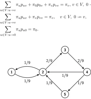
3: 2/11

2: 4/11

1: 2/11 4: 2/11

5: 1/11 1/2

1/2

1/4 1/4

1/2

1/2 1/2

1/4 1/4

1/2 1/2

1/2

Figure 1. A Markov kernel (on edges) with its stationary distribution (on vertices with node’s id) on a simple road network.

Table 1. An example for a Markov kernel on the minimal line digraph of the road network in Fig. 1.

(1,2) (2,3) (3,4) (4,2) (2,1) (4,5) (5,2)

(1,2) 1/2 1/2 0 0 0 0 0

(2,3) 0 1/2 1/2 0 0 0 0

(3,4) 0 0 1/2 1/4 0 1/4 0

(4,2) 0 1/4 0 1/2 1/4 0 0

(2,1) 1/2 0 0 0 1/2 0 0

(4,5) 0 0 0 0 0 1/2 1/2

(5,2) 0 1/4 0 0 1/4 0 1/2

Let𝐴= (𝑎𝑢𝑣)𝑢,𝑣∈𝑉 denote the adjacency matrix of the digraph𝐺, i.e.,𝑎𝑢𝑣= 1 if and only if (𝑢, 𝑣) ∈ 𝐸 and 0 otherwise. The number of directed walks from vertex 𝑢to vertex𝑣 of length 𝑘is the entry in the𝑢-th row and the𝑣-th column of the matrix 𝐴^𝑘. For example, in Fig. 1, the number of directed walks of length 6 from vertex 2 to vertex 4 is 2, see Appendix 7. One can easily check that 𝐺 is strongly connected if and only if there is a positive integer𝑘such that the matrix 𝐼+𝐴+· · ·+𝐴^𝑘 is positive, i.e., all the entries of this matrix are positive. The

(27)

indegree and outdegree of a vertex 𝑣 can be expressed by the adjacency matrix as 𝑑𝑒𝑔⁻(𝑣) =∑︀

𝑢∈𝑉 𝑎𝑢𝑣 and 𝑑𝑒𝑔⁺(𝑣) =∑︀

𝑢∈𝑉 𝑎𝑣𝑢. Let us introduce the vectors 𝑑⁻ := (𝑑𝑒𝑔⁻(𝑣))_𝑣∈𝑉 and 𝑑⁺ := (𝑑𝑒𝑔⁺(𝑣))_𝑣∈𝑉. Then, we have 𝑑⁻ = 𝐴^𝑇1 and 𝑑⁺ =𝐴1where 1:= (1)_𝑣∈𝑉 is the constant unit function. It is well known that the adjacency matrix 𝐴of an aperiodic, strongly connected graph 𝐺is primitive, i.e., irreducible and has only one eigenvalue of maximum modulus. Primitivity is equivalent to the following quasi-positivity: there exists𝑘∈Nsuch that the matrix 𝐴^𝑘 >0, see Section 8.5 in [13].

In order to model the cases when vehicles leave or enter the city, we augment𝑉 by a new ideal vertex 0 and define𝑉 :=𝑉 ∪ {0}, see [12]. Moreover, let𝐸denote the augmentation of𝐸by directed edges(0, 𝑣)and(𝑣,0)for getting into and out of the city, respectively. Note that, for𝐸, it is not allowed to contain the loop(0,0).

The augmentation 𝐺 = (𝑉 , 𝐸)of 𝐺 is called the closure of the road network 𝐺.

For 𝑒= (𝑣, 𝑤)∈𝐸 we also use the notation 𝑣 →𝑤. In what follows, we suppose that there exist𝑢, 𝑣∈𝑉 such that𝑢→0and0→𝑣.

Each definition, including strong connectedness, periodicity, line digraph, given for 𝐺 can be extended for 𝐺 in a natural way. Note that in the augmented line digraph L(𝐺) = (𝑉^′, 𝐸^′)the elements of the edge set𝐸^′can be described by triplets (𝑢, 𝑣, 𝑤), where𝑢, 𝑣, 𝑤∈𝑉 and if𝑣= 0then𝑢, 𝑤̸= 0and if𝑢or𝑤is 0 then𝑣̸= 0 because triplets(0,0, 𝑣),(𝑣,0,0), and(0,0,0)are excluded from𝐸^′. One can easily see that if 𝐺 is strongly connected then its closure 𝐺 is also strongly connected.

Moreover, the strongly connected components of 𝐺, if there exist more than 1, can be connected through the ideal vertex 0, resulting in a strongly connected 𝐺.

Thus, the augmented line digraph will also be strongly connected. Clearly, if G is aperiodic then𝐺is aperiodic too.

In the rest of this paper, it is assumed that the road network is closed by augmenting with the ideal vertex 0.

3. Probability distributions and Markov kernels on road networks

On a road network, two kinds of probability distributions can be defined by considering the set𝑉 or𝐸 as the state space, respectively. However, the Markov kernels on the line road network must be defined with particular care.

A probability distribution (p.d.) on𝑉 is the vector𝜋:= (𝜋𝑣)𝑣∈𝑉 where𝜋𝑣≥0 for all 𝑣 ∈ 𝑉 and ∑︀

𝑣∈𝑉 𝜋𝑣 = 1. We may think of 𝜋𝑣 as the proportion of all vehicles which drive through the crossing𝑣 with respect to all vehicles in the city.

A Markov kernel or transition probability matrix on𝑉 is defined as a real kernel 𝑃 := (𝑝𝑢𝑣)_{𝑢,𝑣∈𝑉} such that𝑝𝑢𝑣≥0for all𝑢, 𝑣∈𝑉 and∑︀

𝑣∈𝑉 𝑝𝑢𝑣= 1for all𝑢∈𝑉. The quantity𝑝𝑢𝑣∈[0,1]is called the transition probability from vertex𝑢to vertex 𝑣. In fact,𝑃 is a stochastic matrix on𝑉 and we assume that its support is the set

(28)

𝐸∪𝑆. The sum condition for Markov kernel𝑃 can be rewritten as:

∑︁

𝑤:𝑣→𝑤

𝑝𝑣𝑤+𝑝𝑣𝑣 = 1, 𝑣∈𝑉. (3.1)

A p.d.𝜋 is a stationary distribution (s.d.) of the kernel𝑃 if∑︀

𝑢∈𝑉 𝜋𝑢𝑝𝑢𝑣=𝜋𝑣

for all𝑣∈𝑉. This so-called global balance equation can be expressed as:

∑︁

𝑢:𝑢→𝑣

𝜋𝑢𝑝𝑢𝑣+𝜋𝑣𝑝𝑣𝑣 =𝜋𝑣, 𝑣∈𝑉. (3.2) Fig. 1 presents a Markov kernel with its s.d. on a simple road network.

Since the vehicles are moving along the road segments of the road network𝐺, it is natural to choose𝐸 to be the state space. In this case, to define probability distributions on the set of vertices again, we have to consider the line digraph L(𝐺) (or ML(𝐺)). Formally, a probability distribution (p.d.) on L(𝐺) is the vector 𝜋^′ := (𝜋_𝑒^′)_𝑒∈𝐸 where 𝜋_𝑒^′ ≥ 0 for all 𝑒 ∈ 𝐸 and ∑︀

𝑒∈𝐸𝜋^′_𝑒 = 1. If we want to emphasize the vertices of the original road network 𝐺, instead of the edges, then the notation 𝜋^′_𝑒=𝜋_𝑢𝑣^′ is also used where 𝑒= (𝑢, 𝑣)∈𝐸. We may think of 𝜋_𝑒^′ as the proportion of the vehicles at the road segment𝑒with respect to all vehicles in the city. Note that𝐺endowed with𝜋^′ is a weighted digraph which is often called a network in itself as well.

A transition probability matrix (or Markov kernel) on𝐸, i.e., on the line digraph L(𝐺), can be defined as a real kernel 𝑃^′ := (𝑝^′_𝑒𝑓)𝑒,𝑓∈𝐸 such that 𝑝^′_𝑒𝑓 ≥0 for all 𝑒, 𝑓 ∈𝐸and∑︀

𝑓∈𝐸𝑝^′_𝑒𝑓 = 1for all𝑒∈𝐸. A p.d.𝜋^′ on𝐸is a s.d. of the kernel𝑃^′if

∑︀

𝑒∈𝐸𝜋^′_𝑒𝑝^′_𝑒𝑓=𝜋^′_𝑓 for all𝑓 ∈𝐸. Since𝐺represents a road system we may suppose that if𝑒̸=𝑓 then𝑝^′_𝑒𝑓>0implies that(𝑒, 𝑓)∈𝐸^′, i.e., there exist𝑢, 𝑣, 𝑤∈𝑉 such that𝑒= (𝑢, 𝑣)and𝑓 = (𝑣, 𝑤), and hence,𝑢→𝑣→𝑤is a walk of length 2. In this case, we use the notation𝑝^′_𝑒𝑓=𝑝^′_𝑢𝑣𝑤as well. In fact,𝑝^′_𝑢𝑣𝑤 denotes the probability that a vehicle on the road segment(𝑢, 𝑣)will go further to the road segment(𝑣, 𝑤) in the next time point. Moreover, in the case of𝑒 =𝑓 = (𝑢, 𝑣), let𝑝^′_𝑒𝑒 =𝑝^′_𝑢𝑣 be the probability that a vehicle remains on the same road segment in the next time point which can be non-zero as well. Thus, since𝑃^′ is a Markov kernel, we have that, for all𝑢→𝑣, ∑︁

𝑤:𝑣→𝑤

𝑝^′_𝑢𝑣𝑤+𝑝^′_𝑢𝑣= 1 (3.3)

and the global balance equation is given as:

∑︁

𝑢:𝑢→𝑣

𝜋^′_𝑢𝑣𝑝^′_𝑢𝑣𝑤+𝜋^′_𝑣𝑤𝑝^′_𝑣𝑤=𝜋^′_𝑣𝑤 (3.4) for all𝑣→𝑤.

An example for the Markov kernel𝑃^′ on the minimal line digraph ML(𝐺) of the road network𝐺in Fig. 1 is shown in Table 1. Fig. 2 shows the unique s.d. 𝜋^′ of the Markov kernel 𝑃^′.

Probability distributions and Markov kernels on the closure𝐺of an open road network𝐺can be defined similarly by considering the set𝑉 or𝐸as the state space,