ECOSYSTEMS AS CLIMATE CONTROLLERS – BIOTIC FEEDBACKS
Á.DRÉGELYI-KISS1*–G.DRÉGELYI-KISS2–L.HUFNAGEL3*
1 Budapest Tech, Bánki Donát Faculty of Mechanical Engineering H-1081 Budapest, Népszínház u. 8., Hungary
(phone: +36-1-666-5332; fax: +36-1-666-5480)
2 University of Pécs, Pollack Mihály Faculty of Engineering, Department of Environmental Engineering
H-7624 Pécs, Boszorkány u. 2.
(phone: +36-72-503-650/3958; fax: +36-72-503-650/3965)
3 Adaptation to the Climate change” Research Group of Hungarian Academy of Sciences H-1118 Budapest, Villányi út 29-43., Hungary
(phone: +36-1-482-6261; fax: +36-1-466-9273)
*Corresponding authors
e-mail: dregelyi.agota@bgk.bmf.hu and leventehufnagel@gmail.com
(Received 15th July 2008; accepted 15th September 2008)
Abstract. There is good evidence that higher global temperature will promote a rise of green house gas levels, implying a positive feedback which will increase the effect of the anthropogenic emissions on global temperatures. Here we present a review about the results which deal with the possible feedbacks between ecosystems and the climate system. There are a lot of types of feedback which are classified.
Some circulation models are compared to each other regarding their role in interactive carbon cycle.
Keywords: climate control, climate change, biotic feedbacks, ecosystem, community
Introduction and aims
It is obvious that human activities could affect the weather and the climate of the Earth, and could change the chemical content of the atmosphere. There is a continuous cycle and flow of inorganic compounds between the atmosphere and the ecosystems, therefore the anthropogenic affects (such as CO2 emission) strongly modify the activities of ecosystems. The modified activities are as follows: fluxes of the photosynthesis, CO2 emission of the soil or the quantity of dissolved organic compounds in the ocean. These activities could have a feedback on the climate controlling the compounds of the atmosphere and therefore on the temperature of the Earth.
The latest IPCC report (Fischlin et al., 2007) points out that a rise of 1,5-2,5 oC in global average temperature makes important changes in the structure and in the working of ecosystems, primarily with negative consequences towards the biodiversity and goods and services of the ecological systems.
The ecosystems could control the climate (precipitation, temperature) in a way that an increase in the atmosphere component (e.g. CO2 concentration) induces the processes in biosphere decrease the amount of that component through biogeochemical cycles. Paleoclimatic researches have proved this control-mechanism for more than 100,000 years. The surplus CO2 content has most likely been absorbed by the ocean,
thus controlling the temperature of the Earth through the green house effect. This feedback is negative therefore the equilibrium is stable.
During the climate control there may be not only negative but positive feedbacks.
One of the most important factors affected the temperature of the Earth is the albedo of the poles. While the average temperature on the Earth is increasing the amount of the arctic ice is decreasing. Therefore the amount of the sunlight reflected back decreases, which warms the surface of the Earth with increasing intensity. This is not the only positive feedback during the control, another good example is the melting of frozen methane hydrate in the tundra.
The most important circle in the biosphere is the global carbon cycle; the changing of the goods, services of ecosystems affected by human interference are examined. This article deals with the ecosystem-climate control and feedbacks.
There are some models in the great climate centres where the composition of the atmosphere is calculated considering the anthropogenic effects with respect to the future. During modelling the control is partly examined, but the climate models are different. In this article the climate-biosphere interaction models are compared regarding to the feedbacks.
Working and modelling of the ecosystems Organization of ecological systems
An ecosystem is a natural unit that includes all plants, the non-living physical factors and their relations to each other (Pásztor et al., 2007). Functions of ecological systems are affected by abiotic environment and biotic factors. The abiotic environment consists of non-physical ecological factors which are the physical and chemical properties of the soil, topographic (e.g. elevation) and climatic components (Moser et al., 1992). Biotic factors are the interactions of organizations (producer, consumer and demolisher organizations), the anthropogenic factors could occur directly and indirectly. Indirectly means a way where the physical, chemical, biological conditions are changed, on the other hand, directly means the effect toward the living creature (e.g. deforestation).
The dynamic unity of habitat and biome is called ecosystem which has a well- defined energy circulation. The ecosystem’s components could be exchanged therefore it is called an opened system. The highest ecosystem is the biosphere where creatures live.
Every ecosystem is characterized by defined assortment and number of species. The ecosystem has not only spatial but temporal expansion, it is in equilibrium, the work of nutrition and energy chain is continuous.
Ecosystem services
Ecosystem services are functions that are enjoyed by mankind. These services can be collected into a few groups (MEA, 2005):
• Provisioning services: the ecosystems take part in producing various products (e.g. food, water, wood)
• Regulating services: climate control, carbon stocks, reconstruction after disaster
• Cultural services: these give aesthetic, spiritual experiences
• Supporting services: primary and secondary production, maintenance of biodiversity, biogeochemical circles
The connection between ecophysiological properties of the plants and the ecosystem’s role are in Table 1.
Table 1. The connection between ecophysiological properties of the plants and the ecosystem’s role (Buchmann, 2002)
Ecophysiological properties of the plants Ecosystem’s role
Photosynthesis, respiration and evaporation Net Ecosystem Exchange of CO2 and H2O Dispersion of carbon (above and under surface of the
land), competition between species, symbiotic connections
Dispersion of fluxes of ecosystems
Growth, aging, falling of leaves Carbon source and sink Mineral resources, climate, life form, plant functional
types, phenology, structure of foliage, succession
Spatial and temporal fluctuation between and in the ecosystems
Energy flux
The basis of the human existence is the photosynthesis and the only energy source is the Sun. Half of the incoming solar radiation ( 342 W/m2) reaches the surface of the Earth (168 W/m2). A little part of this radiation is utilized in photosynthesis (the photosynthetically active radiation, λ=400-770 nm) and the solar energy changes to chemical energy during the photosynthesis:
kJ G
O O
H C O
H
CO 6 Lightplant 6 ' 2850
6 2 + 2 , → 6 12 6 + 2 ∆ =+ (Eq.1)
'
∆G is the change of the standard enthalpy which can be used for profitable work in the plant. The plants convert 1 % of the incoming solar radiation into chemical energy;
this amount maintains the work of the biosphere.
There are three types of photosynthesis according to the bond of the CO2:
• C3 photosynthesis: the CO2 is first incorporated into a 3-carbon compound.
Photosynthesis takes place throughout the leaf. Most plants are C3.
• C4 photosynthesis: the CO2 is first incorporated into a 4-carbon compound.
Photosynthesis takes place in inner cells. C4 plants include several thousand species in at least 19 plant families. Example: forewing saltbush, corn, and many of our summer annual plants.
• CAM photosynthesis: the CO2 is stored in the form of an acid before it is used in photosynthesis. CAM plants include many succulents such as cactuses and agaves and also some orchids and bromeliads.
Some properties of the various photosynthesises are compared in Table 2.
Table 2. Comparison of C3, C4 and CAM photosynthesises (Hopkins, 1999)
Property C3 C4 CAM
Theoretical energy demand (CO2:ATP:NADPH) 1:3:2 1:5:2 1:6,5:2 Transpiration ratio (g H2O/g dry mass) 450-950 250-350 18-125 Speed of photosynthesis (mg bonded CO2/(dm2h)) 15-30 40-80 (low)
Optimum of the temperature (0C) 15-25 30-47 35
Biogeochemical cycles
20 chemical elements take part in the structure of the living creature. Some of them appear in large amount (C, N, P, H, O), others in small quatities (S, K, Na, Ca, Mg, Fe, etc.).
The various biogeochemical cycles exist for every element but they are not separated from each other. The material makes continuous cycling (Szabó I.M, 1989):
• Carbon cycle
In food chain carbon almost always exist as CO2. During the carbon cycle the carbon goes on through the food chain in organic bond and leaves for the atmosphere as CO2. The methane oxidizes fast into CO2, the carbon of the geological sediment are solved by erosion.
• Water cycle
The hydrological cycle are maintained by the solar energy and the gravitation.
More than 80% of the total insolation evaporate water. The atmospheric water vapour condensates and because of the gravitation it falls down like moisture. The energy used during the evaporation process disperses in the atmosphere like heat.
Almost 95% of the water in the Earth is in rocks bonded chemically and physically, does not circulate. 97,3% of the rest is in the oceans, 2,1% is in polar ice and glaciers and the rest is in fresh water (atmospheric water vapour, inland waters, groundwater). The speed of the water cycle between the surface and the atmosphere is very fast, the total cycle is repeated 32 times a year.
• Nitrogen cycle
The largest amount of the nitrogen is in the air but most of the plants are not able to use it directly, it is done by nitrogen-bonded bacteria. The ammonia from the bonded nitrogen becomes nitrates by some other bacteria. These are water soluble feeds for any plant. The nitrates that are not used are converted into nitrites and nitrogen.
• Phosphorus cycle
During the phosphorus cycle the water solves the phosphates from the rocks. The phosphorus is taken up by the plants from aqueous solution of inorganic compounds, the animals take up by eating plants. The bacteria deliver inorganic compounds that contain phosphorus from dead beings. The solved phosphorus from the soil goes into the ocean through fresh water, it gets into fishes, and then through birds of prey get into the mainland as guano.
• Cycle of other biogen elements
There are important structural and regulating role of the Ca cycling, the sulphur is an important component of some amino acid.
The natural material fluxes of the ecosystems are disturbed by human activities.
There are some compounds and radioactive substance that have damaging effect (Sr-90, mercury, DDT, etc.).
Earth-climate interactions
Determining feature of the behaviour of the climatic status is the free variability done by nonlinear inner feedbacks. If the concentration of the carbon dioxide redoubles in a hypothetic atmosphere devoid of feedbacks then +4Wm-2 radiative forcing will be put out, which means an 1,2 °C increase in temperature (Götz, 2004).
The equilibrium climate sensitivity is the change of global surface average temperature in a year in case of redoubling the atmospheric concentration of carbon dioxide (Hegerl et al., 2007). If the equilibrium conditions are not realized then it is called effective climate sensitivity. The climate sensitivity parameter shows how much change in the global surface average temperature in a year is caused by one unit change in radiative forcing (measure unit: °C(Wm-2)-1 ).
According to the IPCC AR4 report the equilibrium climate sensitivity will likely (more than 66% probability) be between 2 oC and 4.5 oC, the best estimation is at about 3 oC. It is unlikely to be under 1.5 oC.
Paleoclimatic research shows that the change in temperature is in proportion with the concentration of the CO2 in the atmosphere during the last 220,000 years (Barnola et al., 1987). The amount of the methane and the temperature are in close relationship (Raynauld et al., 1993). The ratio of the temperature and CO2 concentration is different in various periods. Considering the last 220,000-year period the amount of CO2 increase was 100 ppm, the increase in temperature was 8 oC, which equals to 25 PgC/oC rate.
This sensitivity of the temperature was 40 PgC/oC during the little ice-age (1660-1900), this value is 6 PgC/oC nowadays (1958-1992) (Woodwell et al., 1998).
The main element of the controlling system is the feedback loop. If there is no feedback loop, then the whole effect related to the climate can be calculated from the outer effects:
Y=X, (Eq.2)
where Y is the output parameter, X is the input parameter. If there is one feedback loop, the equation is as follows:
(
g)
X Xg X
Y = + ⋅ = 1+ (Eq.3)
where g is the gain parameter. If there is an infinitive number of repeats, then:
( )
g g X
g g X
Y = + + + + = −
... 1
1 2 3 , if g<1. (Eq.4)
If 1>g>0, then it is called positive feedback, if g<0, then it is negative feedback.
If g>1, then the process is instable, Y=∞.
During the modelling process the general circulation models that are used contain some important feedback mechanisms (Lashof et al., 1997). The most important is the positive feedback of the ice albedo; the second positive feedback is related to the amount of the water vapour. The third feedback is uncertain in its size and direction;
this is the effect of the clouds. The gain of these three feedback loops (g) is between 0,4-0,78 values.
Classification of the feedbacks
The feedbacks can be classified in accordance with their effects (Hartman et al., 2003):
• Effect to the amount of the climate change o Cloud, water vapour feedbacks
The increased CO2 concentration heats the air directly due to the green house effect which takes up more water vapour with higher temperature.
Therefore the heat absorbing ability increases and more uptake of water vapour is caused. The increased amount of the water content of the air- strata could also cause negative feedbacks. The infrared radiation is absorbed by the clouds and heating effect is caused in the rate of the absorbed dose. At the same time the sunshine is reflected back so the
warming is blocked. (Hegerl et al., 2007; Ammann et al., 2007). The degree of the feedback caused by water vapour is difficult to calculate, because the water vapour -in spite of CO2- does not dissipate evenly in the air.
o Ice-albedo feedback
The global warming heats the surface of the Earth, melts the ice barriers.
The white surface of the ice reflects the solar radiation and during its melting the heat is absorbed by the oceans. For this reason the ice- surfaces melt faster and a self-exciter process evolves. (Soden et al., 2006)
o Biogeochemical feedbacks and the carbon cycle
The global carbon cycle and the sulphur cycle contain important feedbacks as well. For example, increase in the concentration of CO2
affects the heat-absorbing ability of the soil. The carbon content of the soil is stored in a sensitive equilibrium, so little change in the temperature is enough for the soil to emit the absorbed CO2.
The transpiration of the plants in rainforests is heightened by the increase of the carbon dioxide concentration. When the stomas are open during the transpiration process a part of their water content is evaporated.
Another positive feedback process is the methane emission from the methane hydrate related to the global warming. Methane hydrate is solid but instable which is originated in the deep sea on low temperature, under high pressure. The basic condition of the formation of methane hydrate is thick sediment in which the methane is formed. If this material comes up to the surface of the oceans then it directly sublimates and accelerates the process of global warming through green house effect.
o Atmospheric chemical feedbacks
The presence of the aerosols decrease the surface temperature of the Earth by 2-3 oC, larger cooling could be felt above the industrialized area, because half of the aerosols in the atmosphere has anthropogenic origin.
The chemical processes of the stratosphere and the troposphere are in contact with temperature, precipitation, circulation and the content of the atmosphere, so the radiation equilibrium of the Earth is affected by them.
• Effect to the transient reaction of the climate
o Heat uptake of the oceans and the circulation feedbacks
Warming of the sea and the above air-strata could heighten the evaporation; i. e. it could increase the water content of the air. Water vapour is the most effective green house gas. If the concentration of the green house gases increases, then warming occurs, the humidity of the atmosphere increases and strengthens the green house effect.
The relation between the atmospheric CO2 and the North Atlantic Deep Water has positive feedback as well.
• Effect to the pattern of the climate change o Hydrological and vegetation feedbacks
These are soil-water feedback, snow-albedo feedback, density of stomas, leaf area feedback, bio-geographic feedbacks.
o Natural variations in the climate system
The El Nino anomaly is caused by the interaction between the atmospheric CO2 and the ocean around the Equator. The feedback between the air, ocean and the atmospheric CO2 concentration is positive.
(Geresdi et al., 2004)
Global carbon cycle
Carbon cycle with natural and anthropogenic effects
The only carbon source of the organic substance of living beings is the atmospheric CO2 gas or the solved CO2 in oceans and waters. This kind of CO2 converts from inorganic substance to organic substance during the photosynthesis.
The atmospheric CO2 concentration has fluctuated between 180 ppm and 300 ppm for 650,000 years according to glacial and interglacial terms. It is generally accepted that the CO2 left for the atmosphere was absorbed by the ocean during the glacial maximum time. Until 1750, the CO2 amount was between 260 and 280 ppm for 10,000 years and the anthropogenic fluctuation of the carbon cycle was negligible compared to the natural effects. The concentration has been continuously increasing since 1750; the last measured value was 380 ppm in 2005. The human activities, the increase of CO2
concentration caused by, consist of:
• Burning of fossil fuels
The world’s whole oil use was 169,362·1015 Btu in 2005, gas use was 107,613·1015 Btu and coal use was 122,562·1015 Btu (1Btu (British Thermal Unit)=1054-1060 J), These values are the equivalent to 5,000 Tg C/year amount.
(EIA, 2006)
• Deforestation
Forests are situated on the 30.3 % of the Earth’s area (39,520,630 km2). The change was
-73,170km2/year between 2000 and 2005 (FAO, 2007). An amount of 1000 Tg C/year goes up to the atmosphere.
• Cement production (Worrell et al., 2001)
In 2005 2284 Tg cement was made while 307 Tg C was emitted. From this 160 Tg C evolved during the producing process and 147 Tg C originated from the energy use.
• Land use change (biomass burning (Ito et al., 2004), industrial growing, converting grass lands into agricultural area)
The biomass burning was 5613 Tg dry substance in 2000: 2814 Tg dry substance is assigned to the opened flames, the rest of these is to the burning of bio-fuels.
Altogether, 2290 Tg C evolved as CO2 and 32.2 Tg C evolved as methane.
Houghton (2006) has examined the size of the land use changing and has found that the emission resulted from the annually change was 2.18±0.8 Pg C/year between 1990 and 1999.
The concentration of the atmospheric methane has an analogous increase. The CH4
concentration was 700 ppb in 1750, while it became as much as 1775 ppb in 2005. The primary sources of this increase are the following ones: (the values related to 1990s, Stern et al., 1998)
• Fossil fuels: 15.2 Tg CH4 (gas burning), 18.0 Tg CH4 (gas supply), 46.3 Tg CH4
(coal mining)
• Moulding the ground: 40.3 Tg CH4
• Peat land, wetland: 200 Tg CH4 (Wang et al., 2004)
• Ruminant animals: 113.1 Tg CH4
• Rice cultivation: 100.8 Tg CH4
Both CO2 and methane play an important role during the global carbon cycle, their continuous fluxes are present among the ocean, the terrestrial biosphere and the atmosphere.
According to the IPCC AR4 report (Fischlin et al., 2007) the carbon flux between the terrestrial biosphere and the atmosphere is 120 Gt C/year (1 Gt = 1Pg = 1000 Tg); it is 70 Gt C/year between the ocean and the atmosphere , considering the natural effects.
Regarding to the anthropogenic effects, the flux between the ocean and the atmosphere increases to 90 Gt C/year.
The increase of the CO2 concentration is 3.2±0.1 Gt C/year in the 1990s. (The rate of increase has become 4.1±0.1 Gt C/year between 2000 and 2005.) The emission is 6.4 Gt C annually due to fossil fuels and cement production, 1.6 Gt C/year due to the land- use change. The ocean takes up 2.2 Gt carbons annually and the terrestrial uptake is 2.6 Gt C/year.
Ocean carbon cycle
One of the absorbent of the CO2 emitted to the atmosphere is the ocean. The ocean slowly reacts to the change of the CO2 content of the atmosphere due to the slow mixing. The ocean CO2 uptake could be decreased by the global warming because the rate of the CO2 dissolution is decreased by the warming of the water-layers close to the surface. The gas dissolves easier in cold water than in warm water, but it dissolves easier in salted sea-water than in pure water because the oceans contain carbonate ions.
There are three types of carbon content in the ocean. The largest amount (98.1%) is in the form of dissolved inorganic compound (DIC), the second (1.85%) is the dissolved organic compound (DOC) and in 0.05% as organic particle (live or dead, particulate organic carbon, POC) (Hegerl et al., 2007). The proportions of the carbon-forms show that abiotic interactions and feedbacks decisively exist in the ocean.
There are three biological and physical pumps for CO2 inside the ocean carbon cycle:
• Dissolving pump
Hydrogen-carbonate arises during the reaction of carbon dioxide and carbonate ion. Because of this reaction the inorganic carbon exists in 0.5 % rate as CO2 gas in the ocean. Since the amount of the CO2 gas is low in the seas, more carbon dioxide could be taken up by the ocean. If the water stays on the surface and warms up, the carbon dioxide comes quickly back to the atmosphere. But if the water delapses in the ocean, the CO2 could be stored thousand years before the circulation makes it come up to the surface. On high latitudes the water of the South Ocean, the Labrador Sea and the North Sea delapses into deepwater. These areas are the most important CO2 sinks of the ocean.
• Organic carbon-pump
The CO2 is taken up by phytoplankton during the photosynthesis and the phytoplankton is eaten by bacteria. Therefore the nutritive and the carbon dioxide come back to the water. This process is the remineralisation which occurs especially in the surface waters. If the phytoplankton die and delapse to the deep water, the CO2 is taken up during the remineralisation and is stored decreasing the effect of the global warming. This type of CO2 delapse happens on high latitudes
because there exist much phytoplankton there, so a great amount of CO2 could sink to the deep water layers.
• CaCO3 dissolving pump
CO2 is bonded by the third pump in the shells and corals. For the first sight it seems that much CO2 is bonded in the form of limestone, but the limestone evolves carbon dioxide gas. The reason is the equilibrium where from two hydrogen-carbonate ions become H2O, CO2 and carbonate ion. The deep water layers are alkaline which is good for the dissolving of the limestone; while surface water layers are acidic which is for the evolving the CO2 gas. The corals live in the warm waters so the evolving gas reaches the surface fast and goes to the atmosphere.
Terrestrial carbon cycle
The net carbon exchange is the difference between the CO2 uptake by the photosynthesis, the respiration of the plants, soil and emissions of other processes (fire, wind, insect attack, deforestation, land use changing). In the last 30 years this net carbon flux was -1.0±0.6 GtC. The processes affected by the carbon cycle in the terrestrial ecosystems are as follows:
• Direct climate effects (precipitation, fluctuation of the temperature): for example the soil respiration increases with increasing temperature
• Change in the composition of the atmosphere (CO2 fertilization, food accumulation, pollution)
There is no agreement among the researchers if the net primer production (NPP) increases due to CO2 fertilization (2/3 of the experiments has proven this). The effect of the fire is the largest to the flux between the terrestrial ecosystems and the atmosphere (biomass and soil become CO2), 1.7-4.1 Gt C/year is the oxidation rate by fires, this is the 3-8% of the terrestrial NPP.
• Effects due to land-use change (deforestation, afforestation, agricultural exercises, their legacy)
Missing sink
The environment is polluted by burning fossil fuels or related to land-use change due to human activities which are important CO2 sources. The CO2 evolves to the atmosphere, dissolves to the oceans, is taken up by the boreal forests and a part of it is missing. (Woodwell et al., 1998; Hegerl et al., 2007). The equilibrium (related to 1990) is that as follows:
Sources Sinks
Fossil
fuels + Land-use
change = Atmosphere + Boreal
forests + Ocean + Missing sink
6.4±0.4 1.6±1.1 3.2±0.1 0.6±0.6 2.2±0.4 2.0±1.1
CO2flux between the atmosphere and the biosphere in Hungary
The residence time of CO2 in the atmosphere is quite long to mix evenly in the whole troposphere of the Earth. Its concentration is approximately the same everywhere except above the source areas, there is little difference between the more polluted northern and southern hemisphere (Haszpra, 2000).
Haszpra and Barcza(2001) show, that the net carbon dioxide uptake was 4.85 t in 1998 and 3.38 t in 1999. The measurement point is in 82 m above the land surface which is related to the nearest 200 km2 area. The anthropogenic emission was 60 million t CO2 (16.4 Mt C) in 2004 (UNFCCC, 2006). The Hungarian ecosystems were net emitters between 2002 and 2006 (in average annually 8 Mt CO2) (Barcza et al., 2008).
CO2 flux data of ecosystems and carbon storing capacity
The various ecosystems take part in the maintenance of the global carbon cycle in several ways. Summarizing the area of the different ecosystems, their carbon storing capacity and NPP values are found in Table 2.
Table 3.Size and NPP values of different ecosystems
Ecosystems Area
[M km2]
Carbon storage NPP (MEA, 2005) [kg C/m2/year]
Deserts 27.7 * 0.01
Steppes and savannas
40 Tropical: 28 (C4) Temperate: 15 (C3/C4)
*
0.34 0.49 Seaside terrestrial
ecosystems
6 * 0.52
Forests 41.6
Tropical: 17.1 Temperate: 10.4
Boreal: 13.7
1640 PgC 0.68
Tundra and arctic regions
5.6 400 PgC
(Gruber et al., 2004)
0.06
Mountains 35.8 * 0.42
Freshwater, wetland 10.3 450 PgC (wetland) 0.36
Oceans, seas 349.3
(14 billiard km3)
38100 PgC (of it 698-708 PgC
organic and 13-23 PgC biomass)
0.15
*: There is no data.
Modelling
The expected changes in climate system could be predicted with segmentalized units of the Earth during simulations. In this respect the parts of the biosphere consist of atmosphere, ocean, behaviour of plants and anthropogenic effects. The atmospheric and the oceanic conditions could be described by the general circulation models (GCM), the vegetation models describe the behaviour of the plants and the forecastcontaining
anthropogenic effects is called emission scenarios. With the collective using of these models it is predicted to long time range what changes are expected in our planet life.
The new generation models are the Earth System Models of Intermediate Complexity (EMIC) which simulate the operation of the Earth.
Emission scenarios
The Intergovernmental Panel of Climate Change published the SRES report (Special Report on Emission Scenarios) related to the anthropogenic emission states (IPCC, 2000). Altogether 40 different SRES scenarios were made in all which were classified into 6 groups according to the various social and economic effects. These categories are the illustrative SRES scenarios which include the following conditions:
• A1 describes a future world with very rapid economic growth, global population that peaks in the mid-century and declines thereafter, and the rapid introduction of new technologies.
• A1FI: intensive fossil fuels
• A1T: non fossil energy sources
• A1B: balance across all sources
• A2 describes a very heterogeneous world in which the main purpose is the self- reliance and the preservation of the local identities. The fertility patterns slowly converged. The economic development is regionally oriented.
• B1describes a convergent world with A1 population, but the economical structure is rapidly changing.
• B2 emphasizes the local solutions to economic, social and environmental sustainability. The growth of the population is increasing like in A2 case, but slower.
The SRES scenarios do not contain more emission-decreasing initiatives but the double aerosol effect is considered; it is calculated with human (e.g. industry, heating, traffic) and natural (e.g. sea salt) effects.
General Circulation Models (GCM)
The general circulation models describe the movements in three dimensional space.
Two types of models exist: the atmospheric (AGCM) and the oceanic general circulation model (OGCM). The AGCM is similar to the weather forecast but the predictions are not in days but in decades or even centuries. Connection between the surface of the Earth and the cryosphera is examined by atmospheric circulation models in three dimensional space. The oceanic circulation model consists of the description the ocean and sea-ice where ocean turbulence, temperature and concentration circumstances are considered.
At the end of the 1960s the atmospheric and the oceanic models are coupled into Atmospheric-Oceanic General Circulation Models (AOGCM) (Bryan, 1969; Manabe, 1969). More well-known AOGCMs (Randall et al., 2007) can be found in Table 4.
Table 4. Coupled atmospheric- oceanic general circulation models and their place related to IPCC AR4 (the numbers are related to web references)
Model (AOGCM) Country Model (AOGCM) Country
BCC-CM1 China [1] FGOALS-g1.0 USA [9]
BCCR-BCM2.0 Norway [2] GFDL-CM2.1 USA [10]
CCSM3 USA [3] GISS USA [11]
CGCM3 Canada [4] INM-CM3.0 Russia [12]
CNRM-CM3 France [5] IPSL-CM4 France[13]
CSIRO-MK3.0 Australia[6] MIROC3 Japan [14]
ECHAM5/MPI-OM Germany [7] MRI-CGCM2.3.2 Japan [15]
ECHO-G Korea, Germany [8] UKMO-HadCM3 Great Britain [16]
Vegetation modelling
The dynamic of the biosphere is described by different vegetation models. The vegetation of the ocean is more simple, therefore the biogeochemical model of the ocean is built in the OGCMs, these are for example OPA, MIT (Peylin et al., 2005). The biogeochemical part consists of the dynamic of plankton and the flux between the ocean and the atmosphere.The dynamic of terrestrial ecosystems are more complex. The processes can be classified into three groups related to their speed; the fastest is the photosynthesis and the respiration, the medium rate changes are processing during the life cycle or season by season and the slowest are the evolutional changes in the genetic structure of organizations. Global vegetation models are developed to connect the vegetation and the climatic conditions interactively (Foley et al., 1996). This connection was based on an asynchronous equilibrium; the models (climate and vegetation) could approach each other with iteration resulting long calculations. The other types of the vegetation models are the Dynamic Global Vegetation Models (DGVM) which simulate transient vegetation dynamic. The changes in the function of the ecosystem (water-, energy- and carbon-balance) and the structure of the vegetation (distribution, physiognomy) are calculated by every model to the effect of the results of the various circulation models. There exist some DGVM and their place of development is shown in Table 5.
Table 5. Some Dynamic Global Vegetation Model
Model (DGVM) Place of development
TRIFFID (Top-down Representation of Interactive Foliage and Flora Including Dynamics)
Hadley Centre, Great Britain
LPJ (Lund Potsdam Jena Dynamic Global Vegetation Model) Potsdam Institute, Germany
HYBRID LSCE, France
IBIS (The Integrated Biosphere Simulator) SAGE, USA SDGVM (Sheffield Dynamic Global Vegetation Model) CTCD, Great Britain
VECODE (Vegetation Continuous Description) Potsdam Institute, Germany
MC1 VEMAP, USA
CLM (Community Land Model) NCAR, USA
In vegetation models there are the following key processes:
• Physiological features : photosynthesis, respiration, stoma conductivity, nutrient uptake
• Structure of the ecosystem: partitioning and growth, phenology, reproduction
• Dynamic feature of vegetation: competition, herbivore, fire and illness, mortality
For modelling the terrestrial carbon cycle a TRIFFID vegetation model was developed by Cox et al., 2001. The net carbon flux of the biosphere is defined by the difference between the CO2 emission related to respiration and uptake related to growth.
In the long run the biosphere is in equilibrium, the amount of the stored carbon is stable.
For a short period there is obviously no equilibrium because of daily, seasonally and annual changes. This equilibrium is influenced by the climate change and anthropogenic emissions. The main elements of the TRIFFID model are:
• Five plant functional types: broadleaves, needle leaves, shrubs, C3 and C4 grass
• Newly originated organic substance (BPP, GPP) and the respiration are defined for every PFT. These parameters depend on climatic conditions (temperature, soil moisture). The difference between them is the net primer production (NPP). This C-content gets to soil through roots, fallen leaves where it is demolished by microbes and gets back to the atmosphere by soil respiration. The difference between NPP and soil respiration is the net ecosystem production (NEP); this amount is stored (positive balance) or released (negative balance) by the biosphere.
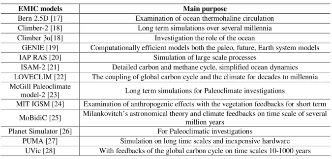
Earth System Model of Intermediate Complexity (EMIC)
Development of EMIC models was made in the frame of International Geosphere- Biosphere Program (Claussen et al., 2002). The summarized models can be seen in Table 6-8 (Claussen, 2005). Among the listed EMIC models the Climber, GENIE, ISAM-2, LOVECLIM and UVic models are suitable for the biotic interactions.
Table 6.Description of EMIC models
EMIC models Main purpose
Bern 2.5D [17] Examination of ocean thermohaline circulation Climber-2 [18] Long term simulations over several millennia Climber 3α[18] Investigation the role of the ocean
GENIE [19] Computationally efficient models both the paleo, future, Earth system models IAP RAS [20] Simulation of large scale processes
ISAM-2 [21] Detailed carbon and methane cycle, simplified ocean dynamics LOVECLIM [22] The coupling of global carbon cycle and the climate for decades to millennia McGill Paleoclimate
model-2 [23] Long term simulations for Paleoclimate investigations
MIT IGSM [24] Examination of anthropogenic effects with the vegetation feedbacks for short term MoBidiC [25] Milankovitch’s astronomical theory and climate feedbacks on time scale of several
million years
Planet Simulator [26] For Paleoclimatic investigations
PUMA [27] Simulation on long time scales and inexpensive hardware UVic [28] With feedbacks of the global carbon cycle on time scales 10-1000 years
Table 7.Details of EMIC models
EMIC Model Atmosphere Ocean Sea ice
Atmosphere-land
contact Ocean biosphere
Bern 2.5D + + + - +
Climber-2 Potsdam-2 MUZON + ASI +
Climber 3α Potsdam-3 GFLD + ASI +
GENIE IGCM+EMBM GOLDSTEIN + - BIOGEM
IAP RAS + + + + -
ISAM-2 + + + OCMIP
LOVECLIM ECBILT CLIO CLIO +
McGill
Paleoclimate model-2 + + + +
MIT IGSM GISS-GCM + -
MoBidiC + + + + +
Planet Simulator PUMA + +
Uvic EMBM GFDL + MOSES2 NPZD
Table 8.Details of EMIC models (continued) EMIC Model Terrestrial
biosphere Ice sheets Interactive
carbon cycle Miscellaneous
Bern 2.5D + - - Season by season cycle
Climber-2 VECODE SICOPOLIS +
Climber 3α VECODE - +
GENIE TRIFFID GLIMMER + Ocean sediment (SEDGEM)
IAP RAS + + -
ISAM-2 + + Biomass burning, biogen
emission
LOVECLIM VECODE + VECODE.LOCH
McGill
Paleoclimate model-2 VECODE +
MIT IGSM CLM -
MoBidiC VECODE + +
Planet Simulator + It is appropriate for other
planets and moons
Uvic TRIFFID UBC
Regional modelling of climate
The method of the regional modelling of climate is the downscalling of the global models. There are some ways to do this:
• Statistical downscalling : There is a connection between the characteristics of global and regional models on the basis of historical behaviour. (Like generally in Hungary (Tóth, 2005).)
• Dynamical procedure: application of high resolution climate models
• Application of different resolution climate models
• Application of limited range climate models
Biotic feedbacks
Anthropogenic warming, rising of the sea-level could continue for centuries due to the scale of climate processes and feedbacks depending on whether the concentration of green house gases are managed to be stabilized (Meehl et al., 2007; Denman et al., 2007). The feedback between climate and carbon cycle gets surplus carbon dioxide to the atmosphere while the climate system is warming. The strength of this feedback is uncertain.
There are two types of natural ecosystems regarding to their place: terrestrial and oceanic ecosystems. Considering the biotic feedbacks larger order of magnitude CO2
gets back to the atmosphere by terrestrial ecosystems.
Biotic feedbacks of oceanic ecosystems
The main element of the oceanic ecosystems and biogeochemical cycle is the carbon.
One of the most important feedback loops of oceanic carbon cycle and climate is the following: the increasing atmospheric CO2 leads to increasing radiative forcing which results higher sea surface temperature (SST) and lower salt-content of sea surface water layers due to stronger hydrological cycle. Therefore it could induce the transformation of the thermohaline circulation in North Atlantic Deep Water, as well as modification of the oceanic carbon cycle, and then the decrease of the transport of the anthropogenic carbon from sea surface into the depth. The decreasing oceanic CO2 uptake could accelerate the increase of atmospheric carbon dioxide.
Other biotic feedback is the production of dimethyl sulphide by phytoplankton.
Dimethyl sulphide oxidizes in the atmosphere and could form aerosols which decrease the global warming (Simo, 2001).
Thirdly, the work of the oceanic organic carbon pump is limited by the amount of mineral resources. Iron and other materials get into the ocean by wind and have a great effect on bond of nitrogen and the amount of the oceanic primer production (Falkowski et al., 1998). Therefore the oceanic net primer production does not increase with the increasing atmospheric CO2 (Zondervan, 2007).
Biotic feedbacks of terrestrial ecosystems
Charney et al., 1975 were the first who examined the effect of ecosystems to the climate. The examination was about feedbacks caused by changes of the surface of the Sahara. Later the global climate models consist of complex effects of land surface and atmosphere. Nowadays it has become important to investigate the effect of the vegetation of terrestrial ecosystems for the climate (Friedlingstein et al., 2006; Meir et al., 2006). As the role of the terrestrial ecology increases in Earth system modelling (EMIC) the feedbacks of the vegetation and soil processes for the climate are determined, and the effect of the land-use change to carbon cycle becomes more clear.
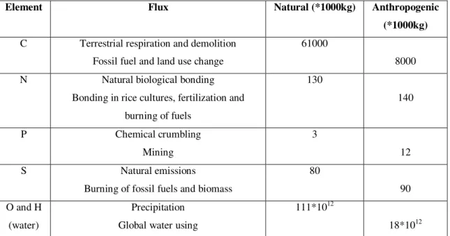
Biotic feedbacks of terrestrial ecosystems to climate are made by various biochemical circles. The global carbon cycle has the largest quantities of fluxes as it can be seen in Table 9.
Table 9. Natural and anthropogenic quantities of chemical element cycles (Falkowski et al., 2000)
Element Flux Natural (*1000kg) Anthropogenic
(*1000kg) C Terrestrial respiration and demolition
Fossil fuel and land use change
61000
8000 N Natural biological bonding
Bonding in rice cultures, fertilization and burning of fuels
130
140
P Chemical crumbling
Mining
3
12
S Natural emissions
Burning of fossil fuels and biomass
80
90 O and H
(water)
Precipitation Global water using
111*1012
18*1012
Three- or four- fold carbon is stored in terrestrial ecosystems than in the atmosphere and more than one eighth of the atmospheric carbon dioxide passes through the ecosystems in a year due to photosynthesis and respiration. Processes of carbon cycle take a feedback to climate which can interpret on two levels: top-down, approaching from the whole biosphere and bottom-up, building from the fundamental biogeochemical processes (see Table 3).
The main feedbacks of carbon cycle and climate are (Luo et al., 2001):
• a positive feedback through photosynthesis, vegetation growth and respiration
• a negative feedback through photosynthesis, vegetation and carbon sequestration
• acclimatization of soil respiration to warming weakens the positive feedback Present day status of the global carbon cycle is important to focus to the following researches (Canadell et al., 2004):
• Determination of forests’ biomass
• Eddy covariance flux net
• Determination of carbon content of soil
• Mineral materials’ transport from rivers to seas
• Measuring the emission of fossil fuels
• N, P, Si, Fe-fluxes to ecosystems
• Non-CO2 emission of ecosystems (CO, CH4, VOC)
• Atmospheric CO2 in space
If these values are available we can size up more precisely the carbon sources and sinks.
Possible biotic feedbacks
CO2 and CH4 are the essential parts of carbon cycle. They make an important role in regulating of ecosystems. Climate could also be affected by biogen aerosols (e.g.
isoprene).
• Equilibrium of photosynthesis and respiration
Increasing atmospheric CO2 (CO2-fertilization) gives negative feedback to climate because plants could take up more carbon which decreases the amount of the carbon dioxide in the atmosphere.
There are many experiments to estimate the effect of the fertilization (CFE).
Lobell and Field, 2008 have found, that an average effect of a 1 ppm increase of CO2 on yields of C3 plants (rice, wheat, maize) is 0.1%. So for an average year 0.14% yield increase is available (with 0.07% dispersion).
• Methane emission of wetlands
There are three important kinds of control for the methane emission: temperature of the soil, depth of water table, size of the opened soil layer. Methane could flow to the atmosphere in several ways, such as with molecular diffusion, bubbling up or through stem of vessel plants. Methane is a green house gas, so reaching the atmosphere the temperature will increase, which results n more methane emissions.
Wetlands and flooded lands (considering the rice lands) spread in 8.6·106 km2 area, an amount of 4.6·106 km2 of which are in tropical and subtropical location (Clarke, 1994). Methane emission is 115 – 237 Tg CH4/year (Gedney et al., 2004).
• Biogen aerosols
Aerosols play an important role in climate system, they absorb, reflect or scatter the incoming solar radiation, so they have a cooling effect. The distribution of several aerosols can be found in Table 10. Many volatile organic compounds get to the atmosphere which gives secondary organic aerosols reacting with hydroxyl residue. There are two classes of SOAs regarding to their genesis: biogen SOA (90%) formed by oxidation of volatile organic compound (VOC) and anthropogenic SOA (10%) formed by oxidation of anthropogenic VOCs. Forests are great isoprene-emitters; the emission can be even 300-500 Mt C/year.
Table 10.Distribution of aerosols (Kanakidou et al., 2005)
Source Total amount (Tg/year)
Biomass burning 54 (45-80)
Fossil fuels 28 (10-30)
Biogen secondary organic aerosol 16 (8-40) Anthropogenic secondary organic aerosol 0.6 (0.3-1.8)
Sum of organic substance 98 (60-150)
Sum of aerosols 800
• Soil respiration
Respiration of soil accelerates with the increase of the temperature, so more CO2
goes to the atmosphere which strengthens the global warming. Raich et al., 2005 examined the amount of the CO2 flux between soil and atmosphere between 1980 and 1994. They have found that the value of the average flux was 80.4 Pg C (79.3-81.8 Pg C) annually; and considering the changes of temperature during a year they have measured 3.3 PgC/year/°C.
• More CO2 content of soil and fallen leaves (Kimball et al., 2001)
Less nitrogen admittance is caused by increased atmospheric carbon dioxide concentration indirectly which decelerates the growth of the plants.
• Effect of warming to plants (Feeley et al., 2007)
More water use is caused by warming, the CO2 uptake and photosynthesis rate is decreased by shift of the temperature from optimum which is originated from less conductivity of stomas. On the other hand, the density and the number of stomas increase on higher temperature and CO2 concentration (Pandeya et al., 2007).
• Fire frequency (Running, 2006)
Occurance of fire becomes more frequent with warming decreasing the carbon content of the terrestrial ecosystems and increasing the concentration of CO2 in the air which increases the temperature.
Coupled carbon cycle-climate models
Feedback of the global carbon cycle is investigated with the help of GCM and EMIC modelling. There are some studies that consider the oceanic carbon cycle’s feedbacks (Joos et al., 1999), only, while EMIC model examines both the oceanic and the terrestrial connections. At first the feedbacks of terrestrial and oceanic ecosystems to climate were simulated by Cox et al., 2000, Hadley Centre, Great Britain. A three- dimensional model has been developed to show, that feedbacks of the global carbon cycle could accelerate the global warming during the 21st century significantly.
During modelling HadCM3 climate model connected with an oceanic carbon cycle model (HadOCC) and a terrestrial dynamic vegetation model (TRIFFID) was used.
Three different runs were made to isolate the effect of climate and the feedback:
• IS92a CO2 emission and fixed vegetation (standard)
• Interactive CO2 emission and dynamic vegetation, supposed that CO2 does not affect the climate (off-line)
• Fully coupled climate-carbon cycle model simulation
The results show that terrestrial carbon sequestration could decrease with global warming; especially in those regions where the increase of the temperature is not advantageous regarding the photosynthesis. In case of low CO2 concentration the direct effect of CO2 dominates and the carbon content of soil and vegetation increases with atmospheric carbon dioxide. Moreover, the increase of the CO2 concentration the carbon content of terrestrial ecosystems begins to decrease because of the respiration of the soil. The intermediate term between the two systems will be about 2050. The CO2
concentration is going to be 980 ppm by 2100 considering the positive feedback of the carbon cycle to the climate.
CO2 uptake of the ocean decreases during the years, the rate will be 5 GtC/year. The different temperatures (due to the increase of the sea surface temperature) hinder to evolve the CO2 gas which decreases the obtainability of nutrient and the net primer production (with 5%).
Dufrense et al., 2002 have made similar simulations in IPSL, France. They have compared the data from Hadley Centre (Friedlingstein et al., 2003). The studies agree in the positive feedback of carbon cycle to climate, but the rate of this feedback is different. They agree that CO2 uptake of the ocean would hardly change during the next century. This is in contrast with the previous, only-ocean models according to which the ocean carbon uptake is decreased by climate change (Joos et al., 1999; Sarmiento et al., 1998).
According to Zeng et al., 2004, Maryland University, USA, the difference between the outputs of the simulations is caused by the determination of the terrestrial carbon content.
The model approach has been improved by C. Jones and his collaborates to reply the results from the Hadley Centre (Jones et al., 2003). The previous used climate model was completed with an interactive carbon cycle considering the cooling effect of the sulphate aerosols, so the overestimation of the CO2 concentration (Cox et al., 2000) was disappeared.
There is a positive feedback of the terrestrial ecosystems to climate but their size is quite uncertain (Govindasamy et al., 2004; Joos et al., 2001). There were investigations to the future in the frame of C4MIP (Coupled Climate-Carbon Cycle Model Intercomparison Project) (Friedlingstein et al., 2006). The model consists of seven coupled ocean-atmosphere general circulation models (OAGCM) and four Earth System models of intermediate complexity (EMIC). These simulations ran for the past and for the 21st century. Every model had the same CO2 emission values for the past and for the future (IPCC SRES A2 scenario).
Most of the models contain the CO2 emissions related to the land-use change but none of the models use the actual Earth surface changes. Therefore the related physical and biogeochemical processes were ignored during the studies.
Two simulations were run with every model: the first is the coupled case where the climate-change affects the carbon cycle and the second one is the non-coupled case where the CO2 was a non-radiant active gas. The difference between the two cases specifies the effect of the climate to the global carbon cycle.
The differences between the various coupled models with the increase of the CO2
concentration will become important by about 2025. Comparing the coupled cases to uncoupled ones the CO2 concentration becomes higher in the former cases. Every model has positive climate-carbon cycle feedback. The amount of this surplus CO2 is quite uncertain; its value will be between 20 ppm and 220 ppm by 2100.
A feedback analysis was performed to CO2 concentration. The effect of the CO2
change to the global average temperature is as follows:
c A
c C
T = ∆
∆ α (Eq.5)
where ∆Tc is the increasing temperature (K), ∆CcA the atmospheric CO2
concentration (ppm), α is the linear transient climate sensitivity, c is related to the coupled model and u is related to the uncoupled case.
The additional warming due to the climate-carbon cycle feedback is:
(
cA Au)
u
c T C C
T −∆ = ∆ −∆
∆ α (Eq.6) So there is an additional 0.1-1.50C warming by 2100 due to the feedback effect.
The positive value of the climate-carbon cycle feedback means that the amount of the permissible emissions should be decreased (Jones et al., 2006).
Conclusion
The environment, the local and the global climate are affected by the ecosystems through the climate-ecosystem feedbacks. There is a great amount of carbon in the living vegetation and the soil like organic substance which could be formed to atmospheric CO2 or methane hereby affecting the climate. CO2 is taken up by terrestrial ecosystems during the photosynthesis and is lost during the respiration process, but
carbon could be emitted like methane, volatile organic compound and solved carbon.
The feedback of the climate-carbon cycle is difficult to determine because of the difficulties of the biological processes.
The biological simplification is essential during the modelling of vegetation processes. It is important to consider more feedbacks to the climate system to decrease the uncertainty of the estimations.
Acknowledgements. This investigation was supported by the projects NKFP 4/037/2001 and the OTKA T042583, VAHAVA project, Adaptation to Climate Change Research Group of Hungarian Academy of Sciences, and Department of Mathematics and Informatics, Corvinus University of Budapest.
REFERENCES
[1] Ammann, C., Joos, F., Schimel, D., Otto-Bliesner, B. and Tomas, R. (2007): Solar influence on climate during the past millennium: Results from transient simulations with the NCAR Climate Simulation Model, Proceedings of the National Academy of Sciences of the United States of America 104 (10) pp.3713-3718.
[2] Barnola, J. M., Raynaud, D., Korotkevich, Y. S., and Lorius, C.(1987): Vostok Ice Core Provides 160,000-Year Record of Atmospheric CO2, Nature 329, 408–414
[3] Barcza Z., Haszpra L., Hidy D., Churkina, G., Horváth L. (2008): Magyarország bioszférikus CO2 mérlegének becslése, Klíma 21 Füzetek, 52, 83-91.
[4] Bryan, K. (1969) Climate and the ocean circulation. III: The ocean model. Mon. Weather Rev. 97 pp. 806-827.
[5] Buchmann, N. (2002): Plant ecophysiology and forest response to global change, Tree Physiol., 22, pp. 1177-1184.
[6] Canadell, J., Ciais, P., Cox, P., Heimann, P. (2004): Quantifying, understanding and managing the carbon cycle in the next decades, Climatic Change, 67, pp. 147-160.
[7] Charney, J., Stone, P.H. and Quirk, W.J. (1975): Drought in Sahara - biogeophysical feedback mechanism, Science, 187, 434-435.
[8] Clarke, R. (1994), The pollution of lakes and reservoirs. UNEP environment library, United Nation Environmental Program, Nairobi, Kenya.
[9] Claussen, M., Mysak, L. A., Weaver, A. J., Crucifix, M., Fichefet, T., Loutre, M.-F., Weber, S. L., Alcamo, J., Alexeev, V. A., Berger, A., Calov, R., Ganopolski, A., Goosse, H., Lohmann, G., Lunkeit, F., Mokhov, I. I., Petoukhov, V., Stone, P., Wang, Z. (2002):
Earth system model of intermediate complexity: closing the gap in the spectrum of climate system models, Climate Dynamics, 18: 579-586.
[10] Claussen, M. (2005): Table of EMICs, http://www.pik-potsdam.de/emics
[11] Cox, P. M., Betts, R. A., Jones, C. D., Spall, S. A., and Totterdell, I. J. (2000):
Acceleration of global warming due to carbon-cycle feedbacks in a coupled climate model, Nature, Vol. 408., pp. 184-187.
[12] Cox, P.M., Betts, R.A., Jones, C.D., Spall, S.A. and Totterdell, I.J. (2001): Modelling Vegetation and the Carbon Cycle as Interactive Elements of the Climate System, Hadley Centre, Technical Note 23
[13] Cramer,W., Bondeau, A.,Woodward, F. I., Prentice, I. C., Betts, R. A., Brovkin,V., Cox, P. M., Fisher, V., Foley, J. A., Friend, A. D., Kucharik, C., Lomas, M. R., Ramankutty, N., Sitch, S., Smith, B., White, A., and Young-Molling, C. (2001): Global response of terrestrial ecosystem structure and function to CO2 and climate change: results from six dynamic global vegetation models, Glob. Change Biol. 7, pp. 357-373.
[14] Denman, K.L., G. Brasseur, A. Chidthaisong, P. Ciais, P.M. Cox, R.E. Dickinson, D.
Hauglustaine, C. Heinze, E. Holland, D. Jacob, U. Lohmann, S Ramachandran, P.L. da Silva Dias, S.C. Wofsy and X. Zhang, 2007: Couplings Between Changes in the Climate