ORIGINAL ARTICLE
Rotation of the age pattern of mortality improvements in the European Union
Péter Vékás1
© The Author(s) 2019
Abstract
Human mortality tends to decline in the long run, which is fortunate for humans, but less so for pension and health insurance schemes and annuity providers. Empirical studies have shown that rates of mortality improvement depend heavily on the age, gender and country in question, and additionally, they also tend to change in time. More specifically, the historical acceleration of mortality decreases among the elderly and a simultaneous slowdown of improvement at younger ages, which are sometimes jointly referred to as the rotation of the age pattern of mortality decline, have been observed in several populations. After a concise summary of the most relevant literature, this paper suggests a simple, largely data-driven methodology with few assumptions for the empirical examination of the rotation phenomenon in historical mortality datasets.
These techniques are then applied on United Nations data from the period between 1950 and 2015 for both genders and all 28 countries of the European Union. The results indicate that rotation has indeed taken place in numerous member states, but its presence is far from universal, and it appears to have been notably more prevalent in populations of women than among men. Life expectancies seem to predict degrees of rotation only in the former Eastern bloc despite prominent literature that suggests otherwise, while increments of life expectancies over the observed period are better predictors of the degrees of rotation in the case of Western European women.
Keywords Mortality·Actuarial science·Demography·European Union·Rotation
I would like to thank the anonymous referees and Patrick Gerland for their valuable comments. This research has been supported by the ÚNKP-17-4-I New National Excellence Program of the Ministry of Human Capacities. This research has been supported by the European Union and Hungary and co-financed by the European Social Fund through the Project EFOP-3.6.2-16-2017-00017, titled
“Sustainable, intelligent and inclusive regional and city models”.
B
Péter Vékáspeter.vekas@uni-corvinus.hu
1 Corvinus University of Budapest, F˝ovám tér 13-15., Room S.201/a, Budapest 1093, Hungary
1 Introduction
Human mortality has decreased significantly since at least the beginning of the past century (Tuljapurkar2000), which has resulted in an unprecedented increase of human life expectancies. Despite its nearly univeral occurence, the speed of mortality decline varies heavily by age, gender and country (Lee2000), and to make things more com- plicated, mortality improvement rates themselves may very well change in time, even for the same triad of the aforementoned variables (Kannisto et al.1994; Horiuchi and Wilmoth1995; Lee and Miller2001; Carter and Prskawetz2001; Rau et al.2008).
1.1 Rotation of the age pattern of mortality decline
More specifically, several authors have noted a historical pattern of diminishing mor- tality decline at relatively younger ages, accompanied by accelerating improvements at more advanced ages (Christensen et al.2009). Li et al. (2013) call this phenomenon the “rotation” of the age pattern of mortality decline, which is captured by a counter- clockwise rotation in Fig.1.
A somewhat simplistic explanation of the rotation is that longevity increases used to be driven by rapidly declining infant and childhood mortality rates (e.g., due to widespread vaccination programs and improved child nutrition)—and to some extent, by improvements in middle-aged mortality—, where spectacular advances are less and less possible, but on the other hand, better medications, nutrition and lifestyle choices for the elderly and costly medical procedures to extend life at higher ages are increasingly available.1It should be noted that the investigation of the causes of the rotation falls outside the scope this paper.
The practical significance of the topic lies in the fact that ignoring rotation in long-term mortality forecasts leads to the systematic underestimation of the old-aged population, which exacerbates longevity risk. This may lead to serious financial consequences for life and health insurers as well as pension schemes.
1.2 Literature overview
Mortality forecasting techniques play a key role in demography, life insurance and pensions. Due to the immense and ever-growing literature on these methods (see e.g. (Booth and Tickle2008) and (Pitacco et al.2009) for comprehensive reviews), an exhaustive overview is not attempted here, but instead, this paper will only focus on sources related to the rotation phenomenon.
1.2.1 The Lee–Carter model
The famous paper of Lee and Carter (1992) has probably been the most important breakthrough in the history of mortality forecasting. The authors model the logarithm of the central mortality rate at agexand calendar yeartas
1 Li et al. (2013) argue that the rotation is more prevalent in developed countries characterized by low mortality, which is consistent with this explanation. Elderly mortality itself is far from homogeneous, and this general description may hold for some age groups and countries and not for others.
Fig. 1 Rotation of the age pattern of mortality decline (stylized illustration)
logmxt =ax+bxkt+εxt, (1) whereaxrepresents the mean of the observed logarithmic central mortality rates for a given age, the time serieskt captures the evolution of the overall level of mortality across time, andbx denotes the speed of mortality decline for every age.
As the parametersbxdo not depend on time, and the time seriesktis overwhelmingly assumed to follow a linear pattern (Tuljapurkar2000), age-specific mortality declines at a constant speed in the Lee–Carter model, and the rate of improvement only depends on the age of the individual in question. The latter implicit assumption of the model has attracted intense scrutiny by the scientific community.
1.2.2 Empirical evidence against constant age-specific improvements
Kannisto et al. (1994) find accelerating mortality improvements between 1950 and 1989 among those aged 80–99 years in 27 countries. Horiuchi and Wilmoth (1995) use Swedish data to demonstrate a shift in mortality improvements from younger towards older ages. Lee and Miller (2001) compare the average rates of mortality improvement by age across the first and second halves of the twentieth century, and observe the shift in mortality improvement from younger to older ages in several countries. Based on this observation, they propose using data from the years after 1950 for the estimation of the Lee–Carter model in order to reduce violations of the time-invariance assumption. Carter and Prskawetz (2001) estimate several Lee–Carter models on Austrian data using different time windows to illustrate the evolution of age-specific mortality decline.2Rau et al. (2008) and Christensen et al. (2009) note that mortality among the oldest old (aged 80 years or more) has overwhelmingly decreased in the second half of the twentieth century in the majority of more than 30 countries, and in some cases, the pace of this decline has accelerated.
2 Additionally, Carter and Prskawetz (2001) also present a procedure to locate structural changes in the time serieskt. Coelho and Nunes (2011) recommend another technique for the same purpose.
1.2.3 The rotated Lee–Carter model
Several approaches have been developed to address the inflexibility of the classic Lee–
Carter framework with respect to the age pattern of mortality decline. Notably, Li et al.
(2013) have managed to incorporate the rotation into the original procedure.3Instead of Eq. (1), they model the logarithms of central mortality rates as
logmxt =ax +B(x,t)kt+εxt. (2) The parameters B(x,t)in Eq. (2) capture the rotation phenomenon by converging smoothly across time from their initial levels corresponding tobx in Eq. (1) to their assumed ultimate levels, as life expectancy at birth advances from an initial threshold to an upper ceiling (the authors propose 80 and 102 years, respectively) in the original model described by Eq. (1). It is important to note that the authors recommend their model for low-mortality countries and very long forecasting horizons, and knowledge of the estimated parameters of the original Lee–Carter model is sufficient to fit the rotated model to data. Ševˇcíková et al. (2016) and Dion et al. (2015) recently incor- porated this technique into population projections for the United Nations Population Division and Statistics Canada, respectively.
1.2.4 Other modeling approaches
Another solution is to capture the rotation by modeling the evolution of age-specific mortality improvement rates instead of mortality rates, as proposed by Haberman and Renshaw (2012) and Mitchell et al. (2013), among others. Bohk-Ewald and Rau (2017) follow this line in a Bayesian framework capable of combining mortality trends of different countries. They demonstrate on British and Danish data that assuming constant age-specific mortality improvement rates may lead to the underestimation of life expectancies at birth, and also apply their framework on U.S. data in Bohk-Ewald and Rau (2016). These approaches are data-driven, as opposed to Li et al. (2013), who impose a somewhat arbitrary process on age-specific mortality improvement rates, as they are of the opinion that empirical evidence for the rotation is too subtle to govern forecasts.
Yet another alternative is the approach of Booth et al. (2002) and Hyndman and Ullah (2007), who recommend using more than one interaction of age- and time- dependent parameters in Eq. (1) in order to capture the non-constant evolution of age- specific mortality improvement rates, which produces so-called multi-factor mortality forecasting models. Bongaarts (2005) proposes a shifting logistic model to describe the transition in the age pattern of mortality decline. Li and Lee (2005), Cairns et al.
(2011), Russolillo et al. (2011) and Hyndman et al. (2013) model mortality rates of several populations in a coherent framework. In a multi-population setting, age-specific rates of mortality improvement are not necessarily constant due to interactions among different populations.
3 Li and Gerland (2011) present an earlier, not fully developed version of this approach.
Further recent developments in this field include De Beer and Janssen (2016), who aim to model the distribution of the age at death by calendar year, and Li and Li (2017), who propose a sequential statistical testing procedure to determine the starting point of the longest plausible estimation base period where the two conditions of the linearity of the time serieskt and the time-invariance of the parametersbx jointly hold, and find that for the majority of the 34 countries examined, this period starts somewhere between 1960 and 1990.
2 Data and methods 2.1 Demographic data
The statistical analysis presented in this paper was performed in R (R Development Core Team2008) using mortality rates, life expectancies at birth and population counts of the 28 members of the European Union.4These indicators are available for both genders, all 28 EU member states, 22 age groups (0, 1–4, 5–9, 10–14, …, 95–99 and 100 years and older) and 13 calendar periods (1950–1955, 1955–1960, …2010–
2015).5The grouping of ages and calendar years smooths the data (akin to moving averages) so that they contain less undesirable random fluctuations. All data are the courtesy of the UN World Population Prospects 2017 (United Nations Population Division2018).
Mortality improvement rates pertaining to age groupx ∈ {x1,x2, . . . ,x22}, calendar period t ∈ {1,2, . . . ,12}, countryc ∈ {c1,c2, . . . ,c28}and genderg ∈ {M,W}, denoted byrxtcgand computed as
rxtcg= −log
mcgx,t+1 mcgxt
(3)
will be used throughout this paper instead of the corresponding mortality ratesmcgxt. 2.2 Measuring rotation
Based on the quantities defined by Eq. (3), acceleration ratesβxcg may be computed for every age groupx∈ {x1,x2, . . . ,x22}and countryc∈ {c1,c2, . . . ,c28}as well as both gendersg∈ {M,W}. Long-term mean acceleration is measured by the slope of the linear trend of mortality improvement rates6:
βxcg=
12
t=1(rxtcg− ¯rxcg)(t− ¯t)
12
t=1(t− ¯t)2 . (4)
4 At the time of writing this paper, the United Kingdom is still officially an EU member state.
5 Every period spans 5 years and starts and ends on July 1 of the respective years.
6 These mean rates of acceleration are averages over a long time period, which may or may not contain intervals that contradict the overall trend, such as in some former socialist countries.
βxcgin Eq. (4) may be interpreted as the mean growth of the mortality improvement rate for age groupx, countrycand gendergover a 5-year period assuming a linear trend. Equation (4) arguably produces more reliable results than computing the mean rate of increase between the starting and end points (akin to the maximum likelihood estimate of the drift parameter of a random walk with drift), since it takes all data points into account and is less sensitive to outliers at the two ends of the data series.
To determine the degree to which rotation has taken place (if at all) for a given country and gender, it has to be examined whether the acceleration of mortality decline has been more pronounced at advanced ages than in the earlier and middle stages of life (possibly characterized by deceleration). In other words, the degree of association between the variables acceleration and age needs to be measured using a plausible statistical technique. As age groupx is an ordinal variable,7and additionally, the association need not be linear for the rotation to take place, the popular Spearman’sρfor rank correlation (computed between the variables age group and acceleration) is chosen as the measure of rotation. Furthermore, as population sizes vary significantly by age group, and more populous age groups should arguably have higher importance in determining the degree of rotation, a commonly used, weighted version of Spearman’s ρ(Pinto da Costa2015) is used, with the respective average population sizesPxcgi over the period 1990–20158as weights:
ρcg=
22
i=1Pxcgi (rank(βxcgi )−μcg)(i−νcg)
22
i=1Pxcgi (rank(βxcgi )−μcg)222
i=1Pxcgi (i−νcg)2 ((c,g)∈ {c1,c2, . . . ,c28} × {M,W}),
(5)
where
μcg=
22
i=1Pxcgi rank(βxcgi )
22
i=1Pxcgi
and νcg=
22
i=1Pxcgi i
22
i=1Pxcgi
are the weighted means (taken over all age groups) of the ranks9of the acceleration rates and the age group indices, respectively.
Additionally, the one-sidedz-test (Pinto da Costa2015) with
H0:ρcg ≤0, H1:ρcg>0 ((c,g)∈ {c1,c2, . . . ,c28} × {M,W}). (6) may be used to test whether degrees of rotation are significantly different from zero.
7 By contrast, time periodtis an interval variable due to its equidistant scale.
8 The reason for choosing this particular period is that it is the longest interval throughout which all EU members have available data for all age groups up to 2015 in United Nations Population Division (2018).
To check sensitivity with respect to the weights, the alternative scenario of using the population sizes from 1990–1995 as weights has been tested. The correlation coefficients between the original and modified degrees of rotation have turned out to be near 0.99 for both men and women, which indicates a lack of sensitivity with respect to the choice of weights.
9 In an increasing order, with average ranks assigned in case of ties.
2.3 Correlations between degrees of rotation and other variables
It is worth examining which variables may predict degrees of rotation ρcg. In this subsection, methods of determining the strengths of association between degrees of rotation and several variables are presented in detail. These associations will be exam- ined in the European Union as a whole, and additionally, within the former Eastern10 and Western blocs separately. The reason for handling these two groups of countries separately is to avoid Simpson’s paradox, which might result from the very different paths of demographic, economic and social development of the two former blocs of countries, especially between 1950 and 1990.
The relationship between degrees of rotation ρcg and gender within bloc b ∈ {EU,W est,East}may be examined by computing and comparing the mean degrees of rotation by gender (weighted by population counts in order to reflect the relative importances of various countries):
ρb(g)=
c∈bρcgPcg
c∈bPcg . (7)
Differences in mean degrees of rotation between the two genders may be tested for significance using the elementary paired-samplesttest with
H0:E[ρb(M)] =E[ρb(W)], H1:E[ρb(M)] =E[ρb(W)] (b∈ {EU,W est,East}), (8) weighted by population counts of the countries.
Additionally, differences in mean degrees of rotation between the two former political blocs may also be investigated separately for men and women by comparing the quantities defined by Eq. (7). To test whether the differences between the two halves of the European Union are significant, the basic independent-samplest test11
H0 :E[ρW est(g)] =E[ρEast(g)], H1:E[ρW est(g)] =E[ρEast(g)] (g∈ {M,W}) (9) may be performed, again weighted by population sizes.
Li et al. (2013) state that rotation is more prevalent in low-mortality countries, and therefore they recommend that the process of rotation in the rotated variant of the Lee–Carter model should only start after the life expectancy at birth has reached a certain threshold (more specifically, they recommend the threshold of 80 years).
To examine the empirical validity of this statement separately for men and women, the strength of the association between degrees of rotationρcgand mean life expectancies at birthe0cg(over the period between 1950 and 2015) is measured using Spearman’s
10 The former Eastern bloc is the group of eleven member states that used to have centrally planned com- mand economies and self-proclaimed communist governments before 1990, comprising Bulgaria, Czechia, Croatia, Estonia, Hungary, Latvia, Lithuania, Poland, Romania, Slovakia and Slovenia.
11 More precisely, its variant not assuming equal variances, which is also known as Welch’sttest.
ρstatistic, weighted by mean population sizes Pcg12. The choice of Spearman’sρis motivated by the fact that the relationship need not be linear, and weighting is applied since population sizes are highly heterogeneous, and countries with small populations should arguably have less importance in determining the strength of the association.
Additionally, to determine which other demographic variables degrees of rotation may depend on, the relationship between degrees of rotationρcgand
– increments of life expectancies at birth between the periods 1950–1955 and 2010–
2015, denoted byΔecg0 , as well as
– remaining life expectancies at the age of 60 years,13denoted byecg60
are examined, again by computing Spearman’s ρ statistic between the variables of interest, weighted by mean population sizes Pcg, by the same argument that more populous countries ought to have more influence on these measures of association.
The reason for choosingΔecg0 is that there used to be significant differences in life expectancies in the 1950s and the patterns of improvements have been different in various countries, whileecg60is another variable of interest because pension providers might only be interested in forecasts for higher ages.
In general, the strength of the association between degrees of rotationρ on the one hand and one of the indicators I ∈ {e0, Δe0,e60} on the other hand, inside bloc b∈ {EU,W est,East}for genderg∈ {M,W}may be measured as
ρbg(I)=
c∈bPcg(rank(ρcg)−αg)(rank(Icg)−βg)
c∈bPcg(rank(ρcg)−αg)2
c∈bPcg(rank(Icg)−βg)2, (10) where
αg=
c∈bPcgrank(ρcg)
c∈bPcg and βg=
c∈bPcgrank(Icg)
c∈bPcg
are the weighted means (taken over all members of the selected group of countries) of the ranks14of the degrees of rotation and the selected indicators, respectively.
To test whether the measures of associationρbg(I)defined by Eq. (10) significantly differ from zero,pvalues of the one-sidedz-test (Pinto da Costa2015) with
H0:ρbg(I)≤0, H1:ρbg(I) >0 (b∈ {EU,W est,East},g∈ {M,W}) will be computed and evaluated for significance throughout the rest of this paper.
12 Again taken over the period between 1990 and 2015, due to some missing data in earlier periods.
13 More specifically, the values from 2012, which are the most recent data available on the website of the United Nations (https://data.un.org). The reason for using this additonal data source is that remaining life expectancies at the age of 60 years are not included in United Nations Population Division (2018).
14 Again in an increasing order, with average ranks assigned in case of ties.
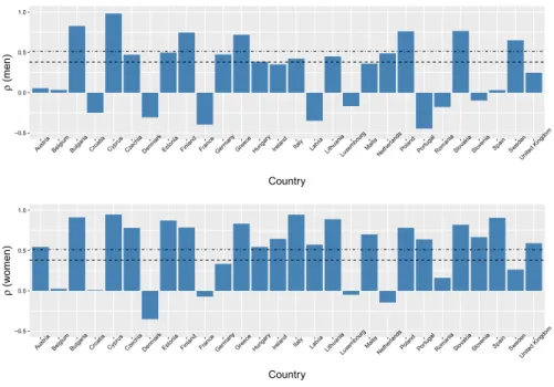
Fig. 2 Degrees of rotation (measured by Spearman’sρ) by country and gender (top: men, bottom: women).
The dashed and dotted-dashed lines denote the one-sided critical values at the 5% and 1% significance levels, respectively
3 Results
3.1 Degrees of rotation by country and gender
Figure2displays degrees of rotation by country and gender, as defined by Eq. (5), alongside the critical values at the 5% and 1% significance levels of the test of the hypotheses defined by Eq. (6). Table5in the Appendix contains the exact numeric values ofρcgas well as thepvalues of the above test by country and gender.
Evidence for rotation is significant at the 5% level in 19 European Union member states for women and 14 countries for men, and only in 11 countries (out of 28) for both genders, which suggests that rotation of the age pattern of mortality decline has been far from universal between 1950 and 2015.15
Apparently, no statistically significant rotation took place in case of either gender in 6 countries (Belgium, Croatia, Denmark, France, Luxembourg and Romania). On the other hand, degrees of rotation are very strongly significant (withp<0.001) for both genders in 6 other EU member states (Bulgaria, Cyprus, Finland, Greece, Poland and Slovakia), with the strongest evidence (ρ≈1 for both men and women) in Cyprus.
15 A stricter testing framework might take into account that 2·28=56 null hypotheses are being tested simultaneously. Hence applying the popular Bonferroni adjustment for controlling the familywise error rate (see Frane2015for a critical discussion), thepvalues below 0.05/56≈0.001, marked by *** in Table5, imply statistical significance at the 5% level. Based on this procedure, statistically significant rotation is detected in only 7 countries for men and 15 member states for women.
Fig. 3 Acceleration rates by age group for men (left) and women (right) in Cyprus (top), Denmark (mid- dle) and Germany (bottom), along with the corresponding LOESS curves. The sizes of the bubbles are proportional to the populations of the corresponding age groups
For the sake of illustration, three selected countries with very different rotation profiles are examined visually in Fig.3in more detail: namely, Cyprus, where evidence for rotation is the strongest for both genders, Denmark, whereρis negative for both men and women, indicating a slight yet somewhat surprising “anti-rotation”, and Germany, the most populous EU member state, which demonstrates weak (if any) evidence for rotation.
The visual pattern is almost perfect in Cyprus, where acceleration rates start from the negative range at age 0, and increase with age thereafter, reaching the positive range around age 40 for men and 20 for women. The weak negative trends in Denmark and the similarly weak positive rotation in Germany are also visible in Fig.3. It should be noted that the acceleration ratesρare weighted by population, which is represented by the sizes of the bubbles in Fig.3. Recognizing the trends with the naked eye is facilitated by LOESS (LOcal regrESSion, a flexible generalization of both moving averages and polynomial regression, Cleveland and Devlin1988) smoothing curves.
The theoretical assumption of time-invariant improvements, which is widely used due to the popularity of the Lee–Carter model, would correspond to horizontal lines at zero acceleration.
The textbook case of Cyprus is further illustrated by Fig. 4, where the pattern of mortality improvements gradually shifted from the solid LOESS curve (1950–1960) to the dashed one (2005–2015). The size of the shift is a nearly perfectly monotone increasing function of age. Charts like Fig.4for Bulgaria, Finland, Greece, Poland
Fig. 4 Rotation of the age pattern of mortality decline for men (left) and women (right) in Cyprus. The solid LOESS curve approximates the pattern of improvement between 1950 and 1960, while the dashed curve displays the new pattern between 2005 and 2015. The sizes of the bubbles are proportional to the populations of the corresponding age groups
and Slovakia yield comparable (even if somewhat more subtle) results, whereas sim- ilar plots for Denmark, France and Luxembourg display weak, barely recognizable tendencies of a clockwise anti-rotation, as captured by the negative values ofρcg. 3.2 Mean degrees of rotation by gender and former political bloc
Table1contains weighted mean degrees of rotation by gender and country group, as defined by Eq. (7). As the weighted mean degree of rotation for women is more than twice as high as the one for men in the European Union as a whole, the results suggest that rotation was considerably more prevalent in female populations than among men between 1950 and 2015. According to the paired-samplest test of the hypotheses defined by Eq. (8), the differences between weighted mean degrees of rotation of men and women are statistically significant in the European Union as a whole as well as within both former political blocs.
On the other hand, even though Eastern member states apparently display higher mean degrees of rotation than coutries in the former Western bloc for both men and women, the differences between these groups are not statistically significant in case of either gender according to thettest with hypotheses defined by Eq. (9).16
16 This occurs due to the high intra-class variances.
Table 1 Weighted mean degrees of rotation by gender and differences between the two genders, with correspondingp values
Gender (region) ρb(g) pvalue
Men (EU) 0.246
Women (EU) 0.498
Gender difference (EU) −0.252 0.001**
Men (West) 0.199
Women (West) 0.466
Gender difference (West) −0.267 0.016*
Men (East) 0.43
Women (East) 0.619
Gender difference (East) −0.189 0.011*
Regional difference (Men) −0.231 0.202 Regional difference (Women) −0.153 0.396
*0.01<p<0.05; **0.001<p<0.01
3.3 Degrees of rotation by life expectancies at birth
Li et al. (2013) state that the rotation of the age pattern of mortality decline is more prevalent in low-mortality countries, and suggest that rotation should only start in their model once a high enough level of the life expectancy at birth (specifically, 80 years) has been reached.
In contrast to this assumption, several European Union member countries display strong evidence in favor of a rotation for both men and women throughout the period between 1950 and 2015, as demonstrated by Fig.2, even though in many cases their life expectancies at birth had still not reached 80 years by 2015 for either males or females (Bulgaria and Slovakia, for example), and numerous other member states with very high life expectancies at birth display no sign of rotation at all (or even to the contrary, such as Denmark and France).
Figure5examines whether rotation has indeed been more prevalent in countries with higher life expectancies at birth. It is apparent in the top row of Fig.5that there is no significant positive trend for either men or women in the European Union as a whole: on the contrary, the linear regression lines have slightly negative slopes, and are nearly horizontal. Based on this figure, the statement of Li et al. (2013) about the relationship between degrees of rotation and life expectancies at birth may hold for Western European men and citizens of both sexes from the former Eastern bloc.
Beyond visual inspection, Table2summarizes the strengths of assocationsρbg(e0), as defined by Eq. (10), between degrees of rotationρcgand life expectancies at birthecg0 alongside their associated pvalues. Table2indicates that the assumption of Li et al.
(2013) only holds among former Eastern bloc countries, and by contrast, degrees of rotation are largely unrelated to life expectancies at birth within the European Union in general and among Western member states in particular.17
17 The same results hold if weighted Pearson’s linear correlation coefficients are used instead of Spear- man’sρ, which increases the validity of these results. In addition, even though there seems to be a positive
Fig. 5 Degrees of rotationρcgas functions of mean life expectancies at birthe0between 1950 and 2015 for men (left) and women (right), in the EU as a whole (top), the former Western bloc (middle) and the former Eastern bloc (bottom). The solid straight lines are linear regression estimates. The sizes of the bubbles are proportional to the (male and female) mid-year populations of the corresponding countries in 2015
Table 2 Strengths of association ρbg(e0)between degrees of rotation and mean life expectancies at birth among all, only Western and only Eastern member states of the European Union, by gender, with one-sided significance levels
Gender (region) ρbg(e0) pvalue
Men (EU) −0.111 0.7
Women (EU) −0.105 0.69
Men (West) 0.043 0.439
Women (West) −0.176 0.735
Men (East) 0.589 0.036∗
Women (East) 0.6 0.032∗
*0.01<p<0.05
3.4 Degrees of rotation by increments of life expectancies at birth
In a similar fashion, Table3displays the strengths of assocationsρbg(Δe0), as defined by Eq. (10), between degrees of rotationρcgand increments of life expectancies at birthΔecg0 as well as the correspondingpvalues. It may be inferred from Table3that degrees of rotation among men are uncorrelated with increments of life expectancies
Footnote 17 continued
trend for Western European men in Fig.5, the standard error around the trend line is too large for the slope coefficient to be statistically significant.
Table 3 Strengths of association ρ(Δe0)between degrees of rotation and life expectancy improvements at birth among all, only Western and only Eastern member states of the European Union, by gender, with one-sided significance levels
Gender (region) ρ(Δe0) pvalue
Men (EU) −0.302 0.929
Women (EU) 0.522 0.003**
Men (West) −0.411 0.939
Women (West) 0.558 0.013*
Men (East) 0.404 0.127
Women (East) 0.296 0.207
*0.01<p<0.05; **0.001<p<0.01
Table 4 Strengths of association ρ(e60)between degrees of rotation and remaining life expectancies at age 60 among all, only Western and only Eastern member states of the European Union, by gender, with one-sided significance levels
Gender (region) ρ(e60) pvalue
Men (EU) −0.14 0.748
Women (EU) 0.209 0.159
Men (West) −0.297 0.86
Women (West) 0.3 0.138
Men (East) 0.46 0.092.
Women (East) −0.439 0.895
.0.05<p<0.1
at birth, while the associations are significant among women, but only in the European Union as a whole and among Western member states, and not inside the former Eastern bloc.
3.5 Degrees of rotation by life expectancies at the age of 60 years
Finally, Table4indicates that degrees of rotation are universally unrelated to remaining life expectancies at age 60 (except for perhaps some very weak evidence in favor of a positive relationship among Eastern European men).
4 Conclusions
Based on detailed data from the period between 1950 and 2015 for both genders and all 28 European Union member states, along with a relatively simple nonparametric, data-driven methodology using only popular, well-known statistical techniques, it is clear that the rotation of the age pattern of mortality improvements has only taken place in part of the 28 members, with only 11 countries displaying statistically significant evidence for rotation at the 5% level in case of both genders, while apparently no rotation at all (or even on the contrary, an anti-rotation) has occurred in a number of EU countries.
The results indicate that the rotation of the age pattern of mortality decline has been notably more prevalent among women than in male populations, in the EU as a whole
as well as within both the former Eastern and Western blocs. This difference has been more significant in the Western half of the Union.
Contrary to Li et al. (2013), the presence and strength of the rotation phenomenon appear to be largely unrelated to mean life expectancies at birth in the European Union as a whole: positive and negative cases appear among both low- and high-mortality countries, and the strength of the assocation between these two variables is apparently statistically negligible. On the other hand, there is significant evidence for a positive relationship between degrees of rotation and life expectancies at birth, as noted by Li et al. (2013), among member states that used to be part of the Eastern Bloc during the Cold War.
Instead of life expectancies at birth, increments of these quantities between the begin- ning and the end of the observation period appear to be better predictors of the degrees of rotation in the case of women in the EU as a whole and the former Western bloc, which has not been noted in the literature.
The questions why the rotation of the age pattern of mortality decline has only taken place in part of the European Union and why it has been more noticeable in time series of female mortality rates deserve closer examination. Most likely, the explanation has to do with the way advances in medicine, lifestyle and nutrition among the elderly have been more prevalent in some countries than in others, especially among women.
Unfortunately, a more thorough investigation of the causes of these findings falls outside the scope of this paper, as it would require an interdisciplinary approach transcending the purely statistical analysis presented here.
It would be desirable to create a multivariate model that explains degrees of rotation using several predictors simultaneously, however, it would require a much larger set of (possibly all) countries as observations in order to produce statistically significant effects.
As the rotation phenomenon may jeopardize the reliability of mortality forecasts for pension schemes as well as life and health insurers, which may lead to severe financial consequences, it is essential to be aware of the possibility of its presence and apply appropriate forecasting procedures that take it into consideration, whenever necessary.
As the immensely popular Lee and Carter (1992) mortality forecasting model ignores rotation, it is advisable to use the particularly promising Li et al. (2013) variant of the original method whenever there is evidence for rotation in the data series. This model variant incorporates a smooth rotation into forecasts, however, it is somewhat inflexible, as the proposed starting point (the age of 80 years) and the speed of the rotation (controlled by the exponent 0.5) are externally given by the authors and are not determined by past data. Making these parameters endogenous, possibly by extending and operationalizing the rotation as presented in this paper, would definitely increase the practical applicability of this excellent method even further.
Acknowledgements Open access funding provided by Corvinus University of Budapest (BCE).
Open Access This article is distributed under the terms of the Creative Commons Attribution 4.0 Interna- tional License (http://creativecommons.org/licenses/by/4.0/), which permits unrestricted use, distribution, and reproduction in any medium, provided you give appropriate credit to the original author(s) and the source, provide a link to the Creative Commons license, and indicate if changes were made.
Appendix
see Table5
Table 5 Degrees of rotationρcgby country and gender and one-sidedpvalues
Men Women
Country ρ pvalue ρ pvalue
Austria 0.055 0.41 0.545 0.006**
Belgium 0.034 0.444 0.025 0.459
Bulgaria 0.829 0*** 0.913 0***
Croatia −0.249 0.852 0.008 0.487
Cyprus 0.983 0*** 0.948 0***
Czechia 0.471 0.018* 0.782 0***
Denmark −0.307 0.904 −0.352 0.935
Estonia 0.498 0.012* 0.873 0***
Finland 0.747 0*** 0.787 0***
France −0.397 0.958 −0.072 0.617
Germany 0.475 0.017* 0.334 0.076.
Greece 0.719 0*** 0.834 0***
Hungary 0.385 0.048* 0.546 0.006**
Ireland 0.351 0.066. 0.645 0.001***
Italy 0.422 0.032* 0.946 0***
Latvia −0.349 0.933 0.573 0.004**
Lithuania 0.45 0.023* 0.889 0***
Luxembourg −0.167 0.75 −0.049 0.58
Malta 0.36 0.06. 0.701 0***
Netherlands 0.488 0.014* −0.144 0.725
Poland 0.762 0*** 0.783 0***
Portugal −0.446 0.976 0.64 0.001***
Romania −0.178 0.771 0.161 0.252
Slovakia 0.766 0*** 0.821 0***
Slovenia −0.097 0.656 0.667 0***
Spain 0.032 0.448 0.907 0***
Sweden 0.651 0.001*** 0.264 0.133
United Kingdom 0.249 0.148 0.592 0.003**
.0.05<p<0.1, *0.01< p<0.05, **0.001<p<0.01, ***p<0.001
References
Bohk-Ewald C, Rau R (2016) Changing mortality patterns and their predictability: the case of the United States. In: Schoen R (ed) Dynamic demographic analysis, vol 39. The Springer series on demographic methods and population analysis. Springer, Berlin.https://doi.org/10.1007/978-3-319-26603-9_5
Bohk-Ewald C, Rau R (2017) Probabilistic mortality forecasting with varying age-specific survival improve- ments. Genus J Popul Sci 73(1):15.https://doi.org/10.1186/s41118-016-0017-8
Bongaarts J (2005) Long-range trends in adult mortality: Models and projection methods. Demography 42(1):23–49.https://doi.org/10.1353/dem.2005.0003
Booth H, Tickle L (2008) Mortality modelling and forecasting: a review of methods. Ann Actuar Sci 3(1–2):3–43.https://doi.org/10.1017/S1748499500000440
Booth H, Maindonald J, Smith L (2002) Applying Lee-Carter under Conditions of Variable Mortality Decline. Population Studies 56(3):325–336.https://doi.org/10.1080/00324720215935
Cairns AJG, Blake D, Dowd K, Coughlan GD, Khalaf-Allah M (2011) Bayesian stochastic mortality modelling for two populations. ASTIN Bull 41(1):29–59
Carter LR, Prskawetz A (2001) Examining structural shifts in mortality using the Lee -Carter method (work- ing paper). Max Planck Institute for Demographic Research.https://www.demogr.mpg.de/Papers/
Working/wp-2001-007.pdf. Accessed 23 Dec 2018
Christensen K, Doblhammer G, Rau R, Vaupel JW (2009) Ageing populations: the challenges ahead. Lancet 374(9696):1196–1208.https://doi.org/10.1016/S0140-6736(09)61460-4
Cleveland WS, Devlin SJ (1988) Locally-weighted regression: an approach to regression analysis by local fitting. J Am Stat Assoc 83(403):596–610.https://doi.org/10.2307/2289282
Coelho E, Nunes LC (2011) Forecasting mortality in the event of a structural change. J R Stat Soc Ser A (Stat Soc) 174:713–736.https://doi.org/10.1111/j.1467-985X.2010.00687.x
De Beer J, Janssen F (2016) A new parametric model to assess delay and compression of mortality. Popul Health Metr 14:46.https://doi.org/10.1186/s12963-016-0113-1
Dion P, Bohnert N, Coulombe S, Martel L (2015) Population Projections for Canada (2013 to 2063), Provinces and Territories (2013 to 2038): technical report on methodology and assumptions. Technical report, Statistics Canada.https://www150.statcan.gc.ca/n1/en/catalogue/91-620-X
Frane A (2015) Are per-family type I error rates relevant in social and behavioral science? J Mod Appl Stat Methods 14(1):12–23.https://doi.org/10.22237/jmasm/1430453040
Haberman S, Renshaw A (2012) Parametric mortality improvement rate modelling and projecting. Insur Math Econ 50(3):309–333.https://doi.org/10.1016/j.insmatheco.2011.11.005
Horiuchi S, Wilmoth JR (1995) The aging of mortality decline. In: Annual meeting of the population Association of America, San Francisco, CA
Hyndman RJ, Ullah MS (2007) Robust forecasting of mortality and fertility rates: a functional data approach.
Comput Stat Data Anal 51(10):4942–4956.https://doi.org/10.1016/j.csda.2006.07.028
Hyndman RJ, Booth H, Yasmeen F (2013) Coherent mortality forecasting: the product-ratio method with functional time series models. Demography 50(1):261–283.https://doi.org/10.1007/s13524-012- 0145-5
Lee RD, Carter LR (1992) Modeling and forecasting US mortality. J Am Stat Assoc 87:659–671.https://
doi.org/10.2307/2290201
Kannisto V, Lauritsen J, Thatcher AR, Vaupel JW (1994) Reductions in mortality at advanced ages: sev- eral decades of evidence from 27 countries. Popul Dev Rev 20(4):793–810.https://doi.org/10.2307/
2137662
Lee R (2000) The Lee–Carter method for forecasting mortality, with various extensions and applications.
North Am Actuar J 4(1):80–93.https://doi.org/10.1080/10920277.2000.10595882
Lee R, Miller T (2001) Evaluating the performance of the Lee–Carter method for forecasting mortality.
Demography 38(4):537–549.https://doi.org/10.1353/dem.2001.0036
Li H, Li JS (2017) Optimizing the Lee–Carter approach in the presence of structural changes in time and age patterns of mortality improvements. Demography 54(3):1073–1095.https://doi.org/10.1007/s13524- 017-0579-x
Li N, Gerland P (2011) Modifying the Lee–Carter method to project mortality changes up to 2100. In:
Annual meeting of the population Association of America, Washington, DC
Li N, Lee R (2005) Coherent mortality forecasts for a group of populations: an extension of the Lee–Carter method. Demography 42(3):575–594.https://doi.org/10.1353/dem.2005.0021
Li N, Lee R, Gerland P (2013) Extending the Lee–Carter method to model the rotation of age patterns of mortality-decline for long-term projection. Demography 50(6):2037–2051.https://doi.org/10.1007/
s13524-013-0232-2
Mitchell D, Brockett P, Mendoza-Arriaga R, Muthuraman K (2013) Modeling and forecasting mortality rates. Insur Math Econ 52(2):275–285.https://doi.org/10.1016/j.insmatheco.2013.01.002
Pinto da Costa J (2015) Rankings and preferences-new results in weighted correlation and weighted principal component analysis with applications. Springer, Berlin. ISBN 978-3-662-48343-5
Pitacco E, Denuit M, Haberman S, Olivieri A (2009) Modelling longevity dynamics for pensions and annuity business. Oxford University Press, Oxford ISBN: 9780199547272
R Development Core Team (2008) R: a language and environment for statistical computing. R Foundation for Statistical Computing, Vienna
Rau R, Soroko E, Jasilionis D, Vaupel JW (2008) Continued reductions in mortality at advanced ages. Popul Dev Rev 34:747–68.https://doi.org/10.1111/j.1728-4457.2008.00249.x
Russolillo M, Giordano G, Haberman S (2011) Extending the Lee–Carter model: a three-way decomposition.
Scand Actuar J 2011(2):96–117.https://doi.org/10.1080/03461231003611933
Ševˇcíková H, Li N, Kantorová V, Gerland P, Raftery AE (2016) Age-specific mortality and fertility rates for probabilistic population projections. In: Schoen R (ed) Dynamic demographic analysis, vol 39. The Springer series on demographic methods and population analysis. Springer, Switzerland, pp 69–89 Tuljapurkar S, Li N, Boe C (2000) A universal pattern of mortality change in the G7 countries. Nature
405(6788):789–792
United Nations Population Division (2018). World population prospects 2017 (maintained by Ševˇcíková, H.).https://CRAN.R-project.org/package=wpp2017Accessed on 12 Jan 2018
Publisher’s Note Springer Nature remains neutral with regard to jurisdictional claims in published maps and institutional affiliations.