An ArcGIS Tool for Modeling the Climate Envelope with Feed-Forward ANN

(1)

This article was downloaded by: [Ákos Bede-Fazekas]

On: 07 April 2015, At: 10:55 Publisher: Taylor & Francis

Informa Ltd Registered in England and Wales Registered Number: 1072954 Registered office: Mortimer House, 37-41 Mortimer Street, London W1T 3JH, UK

Click for updates

Applied Artificial Intelligence: An International Journal

Publication details, including instructions for authors and subscription information:

http://www.tandfonline.com/loi/uaai20

An ArcGIS Tool for Modeling the Climate Envelope with Feed-Forward ANN

Ákos Bede-Fazekas^a, Levente Horváth^b, Attila J. Trájer^cd & Tibor Gregorics^e

a Department of Garden and Open Space Design, Corvinus University of Budapest, Budapest, Hungary

b Department of Mathematics and Informatics, Corvinus University of Budapest, Budapest, Hungary

c Department of Limnology, University of Pannonia, Veszprém, Hungary

d MTA-PE Limnoecology Research Group, Veszprém, Hungary

e Department of Software Technology and Methodology, Eötvös Loránd University, Budapest, Hungary

Published online: 01 Apr 2015.

To cite this article: Ákos Bede-Fazekas, Levente Horváth, Attila J. Trájer & Tibor Gregorics (2015) An ArcGIS Tool for Modeling the Climate Envelope with Feed-Forward ANN, Applied Artificial Intelligence:

An International Journal, 29:3, 233-242, DOI: 10.1080/08839514.2015.1004612 To link to this article: http://dx.doi.org/10.1080/08839514.2015.1004612

PLEASE SCROLL DOWN FOR ARTICLE

Taylor & Francis makes every effort to ensure the accuracy of all the information (the

“Content”) contained in the publications on our platform. However, Taylor & Francis, our agents, and our licensors make no representations or warranties whatsoever as to the accuracy, completeness, or suitability for any purpose of the Content. Any opinions and views expressed in this publication are the opinions and views of the authors, and are not the views of or endorsed by Taylor & Francis. The accuracy of the Content should not be relied upon and should be independently verified with primary sources of information. Taylor and Francis shall not be liable for any losses, actions, claims, proceedings, demands, costs, expenses, damages, and other liabilities whatsoever or howsoever caused arising directly or indirectly in connection with, in relation to or arising out of the use of the Content.

This article may be used for research, teaching, and private study purposes. Any substantial or systematic reproduction, redistribution, reselling, loan, sub-licensing,

(2)

Conditions of access and use can be found at http://www.tandfonline.com/page/terms- and-conditions

Downloaded by [Ákos Bede-Fazekas] at 10:55 07 April 2015

(3)

AN ARCGIS TOOL FOR MODELING THE CLIMATE ENVELOPE WITH FEED-FORWARD ANN

Ákos Bede-Fazekas¹, Levente Horváth², Attila J. Trájer^3,4, and Tibor Gregorics⁵

1Department of Garden and Open Space Design, Corvinus University of Budapest, Budapest, Hungary

2Department of Mathematics and Informatics, Corvinus University of Budapest, Budapest, Hungary

3Department of Limnology, University of Pannonia, Veszprém, Hungary

4MTA-PE Limnoecology Research Group, Veszprém, Hungary

5Department of Software Technology and Methodology, Eötvös Loránd University, Budapest, Hungary

This article is about the development and application of an ESRI ArcGIS tool that implements a multilayer, feed-forward artificial neural network (ANN) to study the climate envelopes of species.

The supervised learning is achieved by a backpropagation algorithm. Based on the distribution and the grids of the climate (and edaphic data) of the reference and future periods, the tool predicts the future potential distribution of the studied species. The trained network can be saved and loaded.

A modeling result based on the distribution of European larch (Larix decidua Mill.) is presented as a case study.

INTRODUCTION

The impact of climate change on the distribution of species can be modeled with climate envelope modeling (CEM), also known as niche-based modeling or correlative modeling (Box1981; Hijmans and Graham2006).

The method is about predicting responses of species to climate change by drawing an envelope around the domain of climatic variables where the given species has been recently found and then identifying areas predicted to fall within that domain under future scenarios (Ibáñez et al.2006).

It hypothesizes that (both present and future) distributions are dependent

Address correspondence to Ákos Bede-Fazekas, Department of Garden and Open Space Design, Corvinus University of Budapest, Villányi út 29-43, H-1118 Budapest, Hungary. E-mail:bfakos@gmail.com

(4)

mostly on the climatic variables (Czúcz 2010). Compared to mechanistic models, CEM tries to find statistical correlations between climate and distribution of species (Elith and Leathwick 2009; Guisan and Zimmermann 2000), and models the future temporal correspondence based on the present spatial correspondence between the variables (Pickett1989). A key advantage of CEM is that there is no requirement for detailed physiological data of species (Pearson et al.2002).

Various methods can be used to determine the climate envelope, including simple regression, distance-based methods, genetic algorithms (GAs), and artificial neural networks (ANNs; Ibáñez et al.2006). The last belong to artificial intelligence (AI) methods that are used less frequently in ecology than statistical approaches because the AI models are considered to be less interpretable and often are called “black-boxes” (Elith et al.2008). A review of the various modeling methods is provided by Guisan and Zimmermann (2000). ANN in CEMs can be mentioned as a method that is relatively new but widely applied (Carpenter et al.1999; Hilbert and Van Den Muyzenberg 1999; Özesmi and Özesmi1999; Hilbert and Ostendorf2001; Pearson et al.

2002; Özesmi et al. 2006; Harrison et al. 2010; Ogawa-Onishi et al. 2010).

ANN-based models are more powerful than multiple regression models when modeling nonlinear relationships (Lek et al.1996). ANNs have proven to be advantageous in many fields of science wherein complex datasets need to be analyzed (Van Leeuwen et al.2012).

The concept of ANN is inspired by the structure and operation of the nervous system. ANN is a machine learning system that has computational units, called neurons, simplification of the human neurons. In general, neurons are organized to lie in layers and are densely connected to each other.

ANN is able to learn and recognize patterns such as climatic patterns that can be found within the distribution of a species. Detailed discussion of the method is provided by Picton (2000) and Van Leeuwen (2012).

PROGRAM DESCRIPTION

The program provides an AI method for CEM in an ESRI ArcGIS¹ 10.0 environment. The program was implemented in Python and is freely accessible through the ESRI tool center (ArcGIS 2013). Based on the distribution (which serves as the base of the presence/absence calculations) and the grids of the climatic, edaphic, topographic, and other data of the reference and future periods (which provide the predictors, or explanatory variables, for the learning and projection phase), the program learns the climatic patterns found within the distribution of the studied species and then predicts the future potential distribution (makes projection). The program

1ArcGIS is a trademark product of the Environmental Systems Research Institute (ESRI) Inc.

(5)

ArcGIS Tool for Modeling the Climate Envelope 235

implements a multilayer, feed-forward ANN to learn the climate envelope of species. Sigmoid, tangent hyperbolic activation function is used. The multilayer topology includes (1) one input layer with the same number of neurons as the number of the given input predictor variables; (2) several hidden layers (the number of the hidden layers and the neurons of the hidden layers can be set); (3) and one output layer with one neuron that is able to estimate the presence/absence in a certain geological point (a point of the grid).

The supervised learning is achieved by a backpropagation algorithm with adjustable learning rate and momentum factor. Multiple predictions can be made in one procedure. The trained network can be saved to and loaded from a file, therefore, training and prediction can be separated.

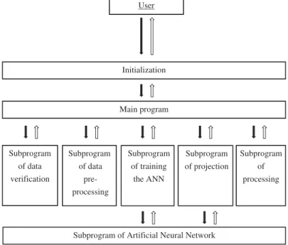
The program has a linear run in a temporal term with five distinguished phases:verifying, data preprocessing, training, projecting, andprocessing phases;

see Figure 1. The verifying phase verifies the input data and the parameters formally and in terms of the content. In case of any problem, the program shows an informative error message and terminates. The data preprocessing and training phases are done if the program was started with the parameter “Should training be done?” being checked. During the data preprocessing, the climatic data are studentized (standardized) for faster training; presence/absence is calculated for every geographic point, and the training pattern is created. Either the entire grid of the reference period can

Initialization

Main program

Subprogram of data verification

User

Subprogram of data

preprocessing

Subprogram of training

the ANN

Subprogram of projection

Subprogram of Artificial Neural Network

Subprogram of processing

FIGURE 1 The logic of the program: the subprogram’s connections to each other and to the user.

(6)

be used for training or a part of it can be selected randomly. In the training phase, the core of the program (the neural network) learns until one of the previously set three termination conditions is satisfied (see them in the next section).

The projecting and processing phases are done if the program was started with the parameter “Should projection be done?” being checked.

During the projection phase the program iterates through the points of the projection grid(s) and the trained neural network makes a projection.

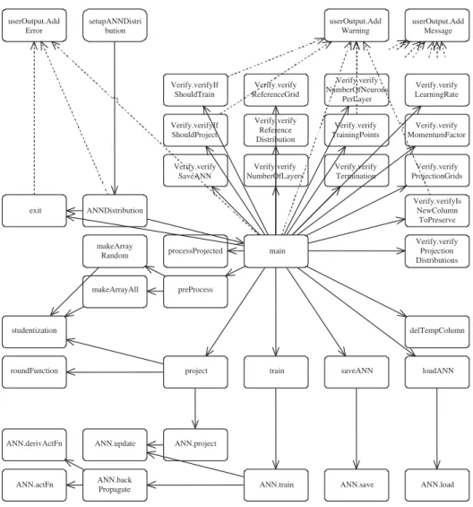
The projection values, typically within the (0;1) interval, are discretized to binary presence/absence data by a manually specified threshold. They can be preserved in a new column of the projection grid. The processing phase is responsible for drawing the potential distribution(s) based on the projection(s) of presence/absence. It is achieved by creating and aggregating Thiessen polygons (Voronoi cells). Detailed structure of the program can be seen inFigure 2.

APPLICATION

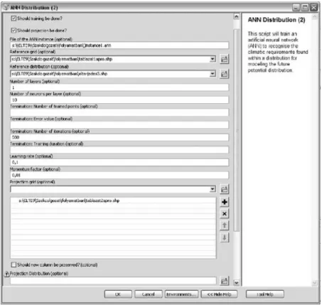
The program can be run (1) as a tool of the ArcToolbox either manually or by Model Builder; (2) or as a script from the Python Window or from other scripts. The program needs several inputs to be given and starting parameters to be set. All the inputs and parameters can be set in the starting window of the tool (Figure 3) or as parameters of the function. After the program has been started, the user cannot affect the running of the program.

In the tool window, the user specifies whether both training and projection should be done or only one or the other. In the case of the training-only or the training-and-prediction mode, the trained network can be saved to a given file. In the case of prediction-only mode, the network previously saved can be loaded from the given file.

In the case of training, the user should set the parameters of the ANN, In other words, the number of hidden layers, the number of neurons per hidden layer, the learning rate, and the momentum factor. A point-type ESRI shapefile (grid) containing the climatic parameters in columns should be loaded as input of the climatic data of the reference period (reference grid). The grid should contain only the climatic parameters and the FID/OID/Shape fields. The user should previously select the appropriate column to avoid high collinearity (detailed information about the phe- nomenon is given by Dormann et al.2013). Another input is the distribution of the species formatted as ESRI polygon-type shapefile (reference distribution). The program bounds the reference distribution to the reference grid. Also, the number of training points and the termination conditions of the training can be set. If no training point number is given, the program

(7)

exit userOutput.Add

Error

userOutput.Add Warning

makeArrayAll preProcess

delTempColumn

saveANN makeArray

Random

studentization

roundFunction

ANN.derivActFn ANN.update

ANN.back Propagate

ANN.project

ANN.actFn

loadANN project

processProjected Verify.verifyIf

ShouldTrain

ANN.load ANN.save

ANN.train Verify.verifyIf

ShouldProject

Verify.verify ReferenceGrid

Verify.verify NumberOfLayers

Verify.verify NumberOfNeurons

PerLayer

Verify.verify TrainingPoints

Verify.verify Termination

Verify.verify LearningRate

Verify.verify MomentumFactor

Verify.verify ProjectionGrids

Verify.verifyIs NewColumn

ToPreserve Verify.verify

Projection Distributions setupANNDistri

bution

Verify.verify SaveANN

Verify.verify Reference Distribution

main ANNDistribution

train

userOutput.Add Message

FIGURE 2 The connection of the program’s functions (userOutput.AddMessage function is excluded, because almost all the other functions call it). The communication toward the user is displayed with dashed lines.

uses the entire reference grid as a training pattern. The optional termination conditions are (1) the number of iterations; (2) the error value to be reached; (3) the training duration in milliseconds.

In the case of projecting, the user should open one or more projection grid(s) with similar structure to that of the reference grid. The column order should be the equivalent of the order within the reference grid. Bias correction of the projection grids should be previously done if necessary.

A checkbox enables setting the calculated presence/absence data, as 1/0 values placed in a new temporary column, if they should be preserved in the projection grids. The user should select as many projection distributions as

(8)

FIGURE 3 The parameterization of the tool at launching.

the number of the projection grids. The program bounds the first grid to the first distribution, and so on. Nonexistent projection distributions are created, while the existing ones are overwritten. The output of the program is the list of the projection distributions that can be handled by Model Builder or by other scripts.

CASE STUDY OFLARIX DECIDUA Aim

A modeling process, including the input data types, the selected parameters, and the modeling result, based on the distribution of European larch (Larix decidua Mill.) is presented as a case study. Although using a more sophisticated CEM and more adequate predictor variables (e.g., soil type, exposure, potential evapotranspiration) could reflect more on the demand of the species, the only aim of the case study was to show how easy the application of the tool is.

(9)

Data Sources

The current (latest update was achieved in 2008) continuous distribution map of European larch (Larix decidua Mill.) was derived from the EUFORGEN digital area database (Euforgen 2009), whereas the discrete (fragmented) observations were ignored. The distribution from 2009 was bound to the reference period of the climate data, because the studied species has a long life cycle and can slowly adapt to the changing climate (Nadezda et al.2006).Larix decidua is one of the most climate-sensitive tree species of the Alps (Carrer and Urbinati2006).

The climatic data were gained from the REMO regional climate model (Hewitt and Griggs 2004); the grid had a 25-km horizontal resolution.

The model REMO is based on the ECHAM5 global climate model and uses the Intergovernmental Panel on Climate Change Special Report on Emissions Scenarios(IPCC SRES) scenario called A1B. The reference period was 1961–1990, the two prediction periods were 2011–2040 and 2041–2070.

The entire European Continent is within the domain of REMO; we used, however, only a part of the grid (25,724 of the 32,300 points). Five climatic predictors were selected, which were averaged in the three periods.

June temperature and precipitation were found to be the best predictors of larch growth in the Southern Alps (Carrer and Urbinati2006). Additionally, mean temperature of January, minimum temperature of September, and precipitation sum of January were used as explanatory variables.

Input Parameters

The selected input parameters were the following. The neural network had 5 hidden layers with 15 neurons per layer. The learning rate and the momentum factor were set to be 0.1 and 0.01, respectively. The entire reference grid was given to the network to be used for training. Only one termination condition was set: the supervised training should be terminated after the tenth iteration.

Result and Discussion

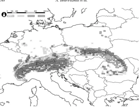
An extract of modeling results can be seen in Figure 4. The modeled potential distributions include parts of Norway and Sweden, which are not displayed. The modeled potential distribution for the reference period shows great similarity to the observed distribution. Although more similarity could be reached in the case of a longer training phase, that could result in an overfitted model. The Cohen’s kappa (Cohen1960) value of the model result for the reference period was 0.4905.

The ratio of the presence data in the entire grid was originally 1.89%

(486/25,724 points). The modeled ratios in 1961–1990, 2011–2040, and

(10)

FIGURE 4 Current distribution (dotted), modeled potential distribution in the reference period (grey), and predicted potential distribution in the periods of 2011–2040 (SW–NE hatch) and 2041–2070 (NW–

SE hatch) of European larch (Larix deciduaMill.), zoomed to Central Europe.

2041–2070 were 2.97, 2.60, and 2.40, respectively. The retraction of the distribution in the Northern Alps is predicted. The model of our previous research (Bede-Fazekas2013) resulted in much larger potential distribution for the reference period and predicted more significant retraction in the Alps.

SUMMARY

The application, applied methods, and example model results of the newly developed ANN Distribution ArcGIS tool are reported to introduce this tool to the community of ecologists. The application of the program is simple because no data transformation, presence/absence calculation, and data migration to statistical software are needed. The program was optimized to the typical data formats of CEM. As far as the authors know, the presented program is the first ANN-based simple CEM tool written to ArcGIS.

Although we stressed the benefits of the tool, we should not forget to mention the challenges. ANN is a black-box method, which is not able to help the ecologists to understand the underlying processes and factors that

(11)

drive the distribution of species; the method can be applied specifically for modeling. This version of the tool lacks automatic parameter setting and regularization scheme, which could prevent the model from becoming overfitted (no statistical measures are calculated during the training phase and, therefore, no automatic calibration can be achieved).

The concept and aim of the program are complex issues and might include many potential developing targets. The main effort for the future version of this program (1) would handle probabilities rather than (or in addition to) binary presence/absences; (2) would continuously model to the reference period to calculate ROC/AUC or Cohen’s kappa values and apply them for early stopping regularization (calibration); (3) would dynamically change the discretization boundary; (4) and would optimize the projecting and processing phases to multicore processors.

FUNDING

ArcGIS is a trademark product of the Environmental Systems Research Institute (ESRI) Inc. The research was supported by the project TÁMOP- 4.2.1/B-09/1/KMR-2010-0005 and TÁMOP 4.2.2.A-1/1/KONV-2012-0064.

The ENSEMBLES data used in this work was funded by the EU FP6 Integrated Project ENSEMBLES (Contract number 505539) whose support is gratefully acknowledged.

REFERENCES

ArcGIS. 2013.ANNDistribution: A tool for modeling the climate envelope with feed-forward artificial neural network.

Available atwww.arcgis.com/home/item.html?id=2c6a49d147b94503b28ff6342e84b4be(accessed October 6, 2013).

Bede-Fazekas, Á., 2013. Negative impact of climate change on the distribution of some conifers.

Hadtudomány23(Suppl.):234–243.

Box, E. O., 1981.Macroclimate and plant forms: An introduction to predictive modelling in phytogeography. The Hague: Dr. W. Junk.

Carpenter, G. A., S. Gopal, S. Macomber, S. Martens, C. E. Woodcock, and J. Franklin. 1999. A neural network method for efficient vegetation mapping.Remote Sensing of the Environment70(3):326–338.

Carrer, M., and C. Urbinati. 2006. Long-term change in the sensitivity of tree-ring growth to climate forcing inLarix decidua. New Phytologist170(4):861–872.

Cohen, J., 1960. A coefficient of agreement for nominal scales.Educational and Psychological Measurement 20(1):37–46.

Czúcz, B., 2010.Modelling the impact of climate change on natural habitats in Hungary(PhD Thesis, Corvinus University of Budapest, Budapest, Hungary).

Dormann, C. F., J. Elith, S. Bacher, C. Buchmann, G. Carl, G. Carré, J. R. García Marquéz, B. Gruber, B.

Lafourcade, P. J. Leitão, T. Münkemüller, C. McClean, P. E. Osborne, B. Reineking, B. Schröder, A.

K. Skidmore, D. Zurell, and S. Lautenbach. 2013. Collinearity: A review of methods to deal with it and a simulation study evaluating their performance.Ecography36(1):27–46.

Elith, J., and J. R. Leathwick. 2009. Species distribution models: Ecological explanation and prediction across space and time.Annual Review of Ecology, Evolution, andSystematics 40(1):677–697.

Elith, J., J. R. Leathwick, and T. Hastie, 2008. A working guide to boosted regression trees.Journal of Animal Ecology77(4):802–813.

(12)

Euforgen, 2009. Distribution map of Europaean larch (Larix decidua). Bioversity International, Rome, Italy.www.euforgen.org/distribution_maps.html(accessed April 1, 2013).

Guisan, A., and N. E. Zimmermann. 2000. Predictive habitat distribution models in ecology.Ecological Modelling135(2–3):147–186.

Harrison, S., E. I. Damschen, and J. B. Grace. 2010. Ecological contingency in the effects of climatic warming on forest herb communities.Proceedings of the National Academy of Sciences USA.

107(45):19362–19367.

Hewitt, C. D., and D. J. Griggs. 2004. Ensembles-based predictions of climate changes and their impacts.

Eos85(52):566.

Hijmans, R. J., and C. H. Graham. 2006. The ability of climate envelope models to predict the effect of climate change on species distributions.Global Change Biology12(12):2272–2281.

Hilbert, D. W., and B. Ostendorf. 2001. The utility of artificial neural networks for modelling the distribution of vegetation in past, present and future climates.Ecological Modelling146(1–3):311–327.

Hilbert, D. W., and J. Van Den Muyzenberg. 1999. Using an artificial neural network to characterize the relative suitability of environments for forest types in a complex tropical vegetation mosaic.Diversity and Distributions5(6):263–274.

Ibáñez, I., J. S. Clark, M. C. Dietze, K. Feeley, M. Hersh, S. Ladeau, A. Mcbride, N. E. Welch, and M. S.

Wolosin. 2006. Predicting biodiversity change: outside the climate envelope, beyond the species- area curve.Ecology87(8):1896–1906.

Lek, S., M. Delacoste, P. Baran, I. Dimopoulos, J. Lauga, and S. Aulagnier. 1996. Application of neural networks to modelling non linear relationships in ecology.Ecological Modelling90(1):39–52.

Nadezda, M. T., E. R. Gerald, and I. P. Elena. 2006. Impacts of climate change on the distribution ofLarix spp. andPinus sylvestrisand their climatypes in Siberia.Mitigation and Adaptation Strategies for Global Change11(4):861–882.

Ogawa-Onishi, Y., P. M. Berry, and N. Tanaka. 2010. Assessing the potential impacts of climate change and their conservation implications in Japan: A case study of conifers. Biological Conservation 143(7):1728–1736.

Özesmi, S. L., and U. Özesmi. 1999. An artificial neural network approach to spatial habitat modelling with interspecific interaction.Ecological Modelling116(1):15–31.

Özesmi, S. L., C. O. Tan, and U. Özesmi. 2006, Methodological issues in building, training, and testing artificial neural networks in ecological applications.Ecological Modelling195(1–2):83–93.

Pearson, R. G., T. P. Dawson, P. M. Berry, and P. A. Harrison. 2002. SPECIES: A spatial evaluation of climate impact on the envelope of species.Ecological Modelling154(3):289–300.

Pickett, S. T. A1989. Space-for-time substitution as an alternative to long-term studies. InLong-term studies in ecology: approaches and alternatives. ed. G. E. Likens, 110–135. New York, NY, USA: Springer.

Picton, P. D. 2000.Neural networks. Basingstoke, UK: Palgrave Macmillan.

Van Leeuwen, B. 2012.Artificial neural networks and geographic information systems for inland excess water classification(PhD Thesis, University of Szeged, Szeged, Hungary).

Van Leeuwen, B., G. Mez˝osi, Z. Tobak, J. Szatmári, and K. Barta. 2012. Identification of inland excess water floodings using an artificial neural network.Carpathian Journal of Earth and Environmental Sciences7(4):173–180.