arXiv:2007.05537v1 [astro-ph.GA] 10 Jul 2020

(1)

APOGEE Data and Spectral Analysis from SDSS Data Release 16:

Seven Years of Observations Including First Results from APOGEE-South

Henrik J¨onsson,^{1, 2} Jon A. Holtzman,³ Carlos Allende Prieto,^{4, 5} Katia Cunha,^{6, 7} D. A. Garc´ıa-Hern´andez,^{4, 5} Sten Hasselquist,^{8, 9} Thomas Masseron,^{4, 5} Yeisson Osorio,^{4, 5} Matthew Shetrone,¹⁰Verne Smith,¹¹

Guy S. Stringfellow,¹²Dmitry Bizyaev,^{13, 14} Bengt Edvardsson,¹⁵ Steven R. Majewski,¹⁶

Szabolcs M´esz´aros,^{17, 18} Diogo Souto,^{19, 20} Olga Zamora,^{4, 5} Rachael L. Beaton,^{21, 22} Jo Bovy,^{23, 24} John Donor,²⁵ Marc H. Pinsonneault,²⁶ Vijith Jacob Poovelil,⁸ and Jennifer Sobeck²⁷

1Materials Science and Applied Mathematics, Malm¨o University, SE-205 06 Malm¨o, Sweden

2Lund Observatory, Department of Astronomy and Theoretical Physics, Lund University, Box 43, SE-22100 Lund, Sweden

3New Mexico State University, Las Cruces, NM 88003, USA

4Instituto de Astrof´ısica de Canarias (IAC), E-38205 La Laguna, Tenerife, Spain

5Universidad de La Laguna, Dpto. Astrof´ısica, E-38206 La Laguna, Tenerife, Spain

6Steward Observatory, The University of Arizona, 933 North Cherry Avenue, Tucson, AZ 85721-0065, USA

7Observatório Nacional, Rua General José Cristino, 77, 20921-400 São Cristóvão, Rio de Janeiro, RJ, Brazil

8Department of Physics & Astronomy, University of Utah, Salt Lake City, UT, 84112, USA

9NSF Astronomy and Astrophysics Postdoctoral Fellow

10University of Texas at Austin, McDonald Observatory, Fort Davis, TX 79734, USA

11National Optical Astronomy Observatory, 950 North Cherry Avenue, Tucson, AZ 85719, USA

12Center for Astrophysics and Space Astronomy, Department of Astrophysical and Planetary Sciences, University of Colorado, Boulder, CO, 80309-0389, USA

13Apache Point Observatory and New Mexico State University, PO Box 59, Sunspot, NM 88349-0059, USA

14Sternberg Astronomical Institute, Moscow State University, Moscow, Russia

15Theoretical Astrophysics, Division of Astronomy & Space Physics, Department of Physics and Astronomy, Uppsala University, Box 516, SE-751 20 Uppsala, Sweden

16Department of Astronomy, University of Virginia, P.O. Box 400325, Charlottesville, VA 22904-4325, USA

17ELTE Eötvös Loránd University, Gothard Astrophysical Observatory, 9700 Szombathely, Szent Imre h. st. 112, Hungary

18MTA-ELTE Exoplanet Research Group, 9700 Szombathely, Szent Imre h. st. 112, Hungary

19Departamento de F´ısica, Universidade Federal de Sergipe, Av. Marechal Rondon, S/N, 49000-000 São Cristóvão, SE, Brazil

20Observat´orio Nacional/MCTIC, R. Gen. Jos´e Cristino, 77, 20921-400, Rio de Janeiro, Brazil

21Department of Astrophysical Sciences, Princeton University, 4 Ivy Lane, Princeton, NJ 08544

22The Observatories of the Carnegie Institution for Science, 813 Santa Barbara St., Pasadena, CA 91101

23David A. Dunlap Department of Astronomy and Astrophysics, University of Toronto, 50 St. George Street, Toronto, ON, M5S 3H4, Canada

24Dunlap Institute for Astronomy and Astrophysics, University of Toronto, 50 St. George Street, Toronto, Ontario, M5S 3H4, Canada

25Department of Physics & Astronomy, Texas Christian University, TCU Box 298840, Fort Worth, TX 76129, USA

26Department of Astronomy, The Ohio State University, 140 West 18th Avenue, Columbus OH 43210, USA

27Department of Astronomy, Box 351580, University of Washington, Seattle, WA 98195, USA

(Received 2020; Revised 2020; Accepted 2020) Submitted to AJ

ABSTRACT

The spectral analysis and data products in Data Release 16 (DR16; December 2019) from the high-resolution near-infrared APOGEE-2/SDSS-IV survey are described. Compared to the previous APOGEE data release (DR14; July 2017), APOGEE DR16 includes about 200 000 new stellar spectra, of which 100 000 are from a new southern APOGEE instrument mounted on the 2.5 m du Pont telescope at Las Campanas Observatory in Chile. DR16 includes all data taken up to August 2018, including

Corresponding author: Henrik J¨onsson henrikj@astro.lu.se

arXiv:2007.05537v1 [astro-ph.GA] 10 Jul 2020

(2)

data released in previous data releases. All of the data have been re-reduced and re-analyzed using the latest pipelines, resulting in a total of 473 307 spectra of 437 445 stars. Changes to the analysis methods for this release include, but are not limited to, the use of MARCS model atmospheres for calculation of the entire main grid of synthetic spectra used in the analysis, a new method for filling “holes” in the grids due to unconverged model atmospheres, and a new scheme for continuum normalization.

Abundances of the neutron capture element Ce are included for the first time. A new scheme for estimating uncertainties of the derived quantities using stars with multiple observations has been applied, and calibrated values of surface gravities for dwarf stars are now supplied. Compared to DR14, the radial velocities derived for this release more closely match those in the Gaia DR2 data base, and a clear improvement in the spectral analysis of the coolest giants can be seen. The reduced spectra as well as the result of the analysis can be downloaded using links provided in the SDSS DR16 web page.

1. INTRODUCTION

The Apache Point Observatory Galactic Evolution Experiment (APOGEE,Majewski et al. 2017) was originally an infrared stellar spectroscopic survey within SDSS-III (Eisenstein et al. 2011, henceforth APOGEE- 1), and APOGEE-2 is the continuation of the same program within SDSS-IV (Blanton et al. 2017). For every SDSS data release that has included APOGEE data (beginning with DR10), the survey has re-analyzed the previous (APOGEE-1 and APOGEE-2) spectra using the most up-to-date version of the data reduction and analysis pipelines, and hence SDSS-IV/APOGEE- 2 data releases include data taken during the SDSS- III/APOGEE-1 project. In this paper, we present the data and data analysis from the sixteenth SDSS Data Release (DR16). Henceforth, we will use “APOGEE”

to refer to the full data set that includes data from both SDSS-III and SDSS-IV. The selection of targets for the stars observed within the APOGEE-1 period is described inZasowski et al.(2013) and the selection for those in APOGEE-2 are described in Zasowski et al.

(2017), R. Beaton et al. (in prep), and F. Santana et al.

(in prep).

In previous data releases, all main survey data have been collected using the APOGEE-N (north) instrument (Wilson et al. 2019) in combination with the 2.5 m Sloan Foundation telescope (Gunn et al. 2006) at Apache Point Observatory in New Mexico (APO). Henceforth this instrument/telescope combination will be referred to as “APO 2.5 m”. Using this combination, 300 spectra of different objects within a 3 degree (diameter) field on the sky can be collected. In addition, some spectra have been collected using the NMSU 1.0 m telescope at APO using the same APOGEE instrument with a single object fiber feed (“APO 1.0 m”). With this instrument/telescope combination, only one star can be observed at a time, and it has mainly been used to observe bright targets for validation of the APOGEE spectral analysis. Since February 2017 another, nearly identical APOGEE spectrograph (Wilson et al. 2019), APOGEE-

S (south), has been operating at the 2.5 m du Pont telescope (Bowen & Vaughan 1973) at Las Campanas Ob- servatory in Chile (“LCO 2.5 m”), enabling observations of the southern sky not accessible from APO. Given the different focal ratio of the du Pont telescope, the field of view is limited to 2 degrees in diameter. DR16 is the first data release of APOGEE that includes data from the southern instrument/telescope.

Within the APOGEE-1 and APOGEE-2 surveys, sub- projects – and hence their observations – are classified as core, goal, or ancillary and given different observa- tional priorities. Thecoreprograms focus on theGalac- tic Evolution Experiment, while the goal and ancillary projects have more specialized science goals. Within the core program are the APOGEE main survey targets, which are chosen using a well-defined, relatively simple, color and magnitude selection function that is designed to target cooler stars. In addition to the survey targets, the current dataset also contains data from externalcontributed programs taken with the southern instrument by the Carnegie Observatories and Chilean community who have access to the duPont telescope;

these are “classical” observing programs vetted through a Time Allocation Committee outside of SDSS for which the individuals granted time are responsible for prepar- ing the observations, but have agreed to have their data included in the SDSS releases. The final target selection for APOGEE-2N (North, APO) and APOGEE-2S (South, LCO) will be presented in R. Beaton et al. (in prep) and F. Santana et al. (in prep), respectively.

2. THE SCOPE OF DR16

DR16 contains high-resolution (R∼22 500), multi- plexed, near-infrared (15 140-16 940 ˚A) spectra for about 430 000 stars covering both the northern and southern sky, from which radial velocities, stellar parameters, and chemical abundances of up to 26 species are determined.

Figure 1 shows the DR16 coverage of the sky compared to the sky coverage of the previous APOGEE data release (DR14; APOGEE did not release any new

(3)

data in the SDSS DR15). The circular footprints of the 300 simultaneous stellar spectral observations that are made with APO 2.5 m and LCO 2.5 m can clearly be seen (henceforth “fields”), as well as the more scattered, single star APO 1.0 m observations. The targets that meet the main survey target selection criteria (which can be identified in the release by objects that have a EX- TRATARG bitmask¹value of 0) have been marked with a darker color. Note that these stars mightalsobe “spe- cial targets” from goal, ancillary, or external programs, that happen to meet the survey criteria, see Zasowski et al.(2013,2017) for details.

An overview of the different APOGEE data releases is shown in Table 1². DR16 contains spectra and derived data for 437 445 individual stars. Most stars are observed in multiple observations, “visits.” While individual radial velocities are determined for each visit, the visits are combined for the stellar parameter and abundance analysis. However, some stars are observed as part of multiple fields, i.e., using different instrument/telescope combinations and/or in more than one field center position, and these are analyzed separately;

hence some stars have more than one entry in the final (fits) table of analysis results (the allStar-file³). This is the reason that the total number of spectra in Table 1 has 473 307 entries for DR16⁴.

For DR16, we decided to remove the spectra observed during the commissioning of the APOGEE-N instrument in winter-spring 2011, since these are of significantly lower resolution due to initial optical alignment issues with the instrument, and therefore do not meet the survey requirements. Most of these stars have been re-observed after the performance of the instrument was improved in the summer of 2011, but we note that this results in some objects that appeared in previous releases but do not appear in DR16.

For most objects, multiple visits are made to build up signal-to-noise (S/N) and to provide multiple radial velocity (RV) measurements. However, all data taken up to the cutoff date for a given data release are included, even if all of the planned visits for some fields have not been completed. Given this and other issues that might affect S/N, not all spectra in a data release reach the tar-

1https://www.sdss.org/dr16/algorithms/bitmasks/

2 The first release, DR10, is excluded in the table since this release only included stellar parameters. DR11 and DR15 did not include any new APOGEE data/analysis.

3https://www.sdss.org/dr16/irspec/spectro data/

4 For the stars with multiple entries in the allStar-file, we aid the user by choosing a preferred spectrum of those stars based on the S/N, by setting bit 4 in the EXTRATARG bitmask for the non-preferred spectra.

get S/N of 100 per half-resolution element. For DR16, 67 503 spectra (14%) have S/N<70 and 19 796 spectra (4%) have S/N<30. These spectra are flagged with the SN WARN and SN BAD bits, respectively, set in the ASPCAPFLAG bitmask in the allStar-file.

3. DATA REDUCTION

The basics of the reduction pipeline are described in Nidever et al.(2015), with subsequent updates for DR13 and DR14 described in Holtzman et al.(2018). While the data reduction for DR16 (version r12) is similar to that used for the previous data release (DR14, version r8), some updates/changes have been made:

• Motivated by different cosmetic issues in the detectors for APOGEE-S, some changes were implemented in the construction of pixel masks to improve masking of bad pixels, making the masking more conservative to avoid some poor quality data not being masked, as seen for some spectra in previous data releases.

• Several changes were made to provide reduced spectra with approximate relative flux calibration, which was not done for DR14. These include changes in the removal of illumination spectral sig- natures in the internal and dome flats, and the subsequent use of hot stars on each plate to provide an approximate relative flux calibration.

• Improvements were made to the wavelength calibration routines: rather than using single wavelength calibration frames for the entire survey, a wavelength solution is determined separately for each year of observation from multiple wavelength calibration frames taken throughout the year. The wavelength calibration routines now allow for small relative motions of the three detectors, which appear to occur when the detector assembly is moved to provide for observations at two different detector dither positions as a means to improve sampling of the spectra.

• The list of sky lines used to determine the wavelength zero-points of each observation was revised slightly, and the wavelength offsets calculated for each observation (necessary because of the dither- ing) allow for the small relative motions of the three detectors. The revised sky line list was also used for the determination of the line spread function (LSF).

• A new grid of synthetic spectra used for radial velocity determination was constructed using a sub-

(4)

Figure 1. The left figure shows the APOGEE sky coverage of SDSS DR14, while the right figure shows the coverage of DR16.

Observations made with APO 2.5 m are plotted in blue, observations made with LCO 2.5 m are plotted in red, and observations made with APO 1.0 m are plotted as small black dots. Observations not meeting the main survey target selection criteria are marked with lighter colors. Note in particular how the new southern instrument delivers a more complete coverage of the bulge region (in the center of the plots), and enables the Magellanic clouds to be observed (the large collection of red points in the lower right-hand corner of the right panel).

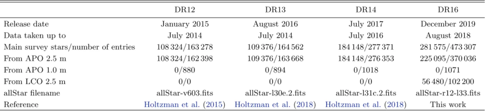
Table 1. The APOGEE data releases that include abundance determinations (the first APOGEE release, DR10, included only stellar parameters – seeM´esz´aros et al.(2013) – and APOGEE did not release any new data/analysis in the SDSS-III/IV Data Releases 11 and 15). The number of spectra are listed as main survey targetstars/number ofentries in the corresponding allStar-file, see text for details.

DR12 DR13 DR14 DR16

Release date January 2015 August 2016 July 2017 December 2019

Data taken up to July 2014 July 2014 July 2016 August 2018

Main survey stars/number of entries 108 324/163 278 109 376/164 562 184 148/277 371 281 575/473 307

From APO 2.5 m 108 324/162 398 109 376/163 668 184 148/276 353 225 095/370 036

From APO 1.0 m 0/880 0/894 0/1018 0/1071

From LCO 2.5 m 0/0 0/0 0/0 56 480/102 200

allStar filename allStar-v603.fits allStar-l30e.2.fits allStar-l31c.2.fits allStar-r12-l33.fits Reference Holtzman et al.(2015) Holtzman et al.(2018) Holtzman et al.(2018) This work

set of the synthetic grid used for stellar parameter and abundance determination (see Section 4).

• Comparison of each stellar spectrum against the full RV grid was made for RV determination; DR14 had implemented a restriction of the grid based on the observed color of each star, but this was found to lead to some spurious results.

• Improvements were made for the removal of telluric lines in APO 1.0 m spectra, which need to be handled differently than the normal multi object observations since there are no concurrent observations of hot stars.

For DR16, the organization of the reduced data files has changed from that of previous data releases, to a

large extent because of the addition of the LCO data;

reductions are now separated into subdirectories based on the telescope and the field names. The data file organization is described in the SDSS data model⁵. Reduced data frames and spectra are available for download from the SDSS Science Archive Server⁶; the Science Archive Webapp⁷provides a convenient interface to inspect and download spectra for individual and groups of objects.

4. SPECTRAL ANALYSIS

The heart of the spectral analysis of the APOGEE Stellar Parameter and Chemical Abundance Pipeline

5https://www.sdss.org/dr16/irspec/spectro data/

6https://data.sdss.org/sas/dr16/

7https://dr16.sdss.org/

(5)

(ASPCAP, Garc´ıa P´erez et al. 2016) is the program FERRE⁸ (Allende Prieto et al. 2006), which interpo- lates in a pre-computed grid of synthetic spectra to find the best fitting stellar parameters describing an observed spectrum. Once the stellar parameters have been determined, these (including the “abundance parameters”, [α/M], [C/M], [N/M], see Section 5.2) are held fixed and the abundances are determined with fits using the same grids, but restricted to windows of the spectra that include lines of the element of interest. A devel- opment of FERRE motivated by the large spectral grids of APOGEE is the use of principal component analysis (PCA) to compress the grids; the actual interpola- tions are performed in the PCA coefficients to speed up the calculations (see Section4.5). This type of analysis has been used in all previous APOGEE data releases, and has been previously described inGarc´ıa P´erez et al.

(2016), with updates in Holtzman et al. (2018). In this section we focus on DR16-specific updates/changes made to previous iterations of ASPCAP described in those papers.

4.1. Main stellar atmospheric models

In DR14, ATLAS-9 atmospheric models (Kurucz 1979, and updates) were used to generate synthetic spectra, but a grid of cooler MARCS-models (Gustafs- son et al. 2008) was used forT_eff<3500 K, seeM´esz´aros et al. (2012); Zamora et al. (2015); Holtzman et al.

(2018) for details. For DR16, we (B. Edvardsson) computed a new all-MARCS grid of atmospheric models and these were used exclusively (apart from stars with Teff> 8000 K, see Section 4.4). The main motivation for this change is to avoid the discontinuity between the two subgrids seen in DR14-data (compare Figure 11);

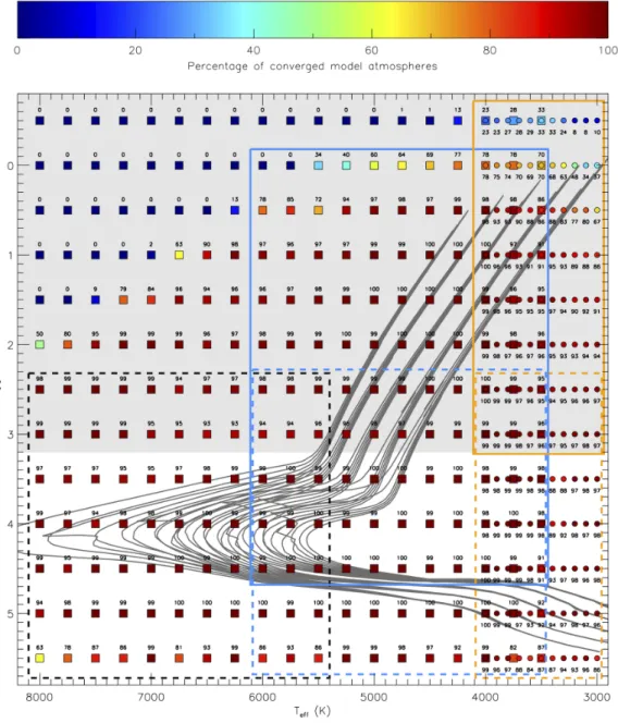
MARCS models are required to handle the lowest effective temperatures of our targets since the ATLAS grid has a lower limit of 3500 K. Additionally, a transition to MARCS models has made it possible to use spherical models for logg≤ 3. Figure 2 shows the location of models in theT_eff-logg-plane; the grid has finer spacing for 3000 K ≤Teff≤ 4000 K where the model structure changes more with specifiedTeff.

For every grid point shown in the T_eff-logg plane [M/H] is varied from -2.50 to +1.00 in steps of 0.25 dex (15 steps), [α/Fe] (which includes changes in O, Ne, Mg, Si, S, Ar, Ca, and Ti) is varied between -1.0 to +1.0 in steps of 0.25 dex (9 steps) and [C/Fe] is varied between -1.00 to +1.00 in steps of 0.25 dex (9 steps), meaning that every grid point shown in Figure2in fact represents 1215 model atmospheres. This adds up to 300 105 at-

8http://github.com/callendeprieto/ferre

tempted calculated atmospheric models for the warmer grid, and 173 745 models in the cooler, finer spaced grid, and 442 260 models in total (there are some overlapping grid points in the two grids, see Figure 2). However, only 358 123 of these models converged, leading to 84 137 holes in our grid. The fraction of holes in theTeff-loggplane is shown in the small numbers as well as in the color-coding in Figure 2. In general, most of the holes are in regions of the grid where we do not expect many stars, for example with high Teff and low logg, and/or with elemental abundances near the grid edges in the abundance dimension in question. However, of particular interest is that of the models with logg=−0.5, only 1% of all models converged.

The holes in the model atmospheric grid obviously translate to holes in the grid of synthetic spectra, but as described in Section 4.3.1, these holes are filled before the analysis of data using Radial Basis Functions (RBF) interpolation (and extrapolation) in flux-space.

4.2. Line list

In DR14 we used the atomic and molecular line lists described inShetrone et al.(2015) (this set of lists is internally labeled as 20150714 based on the date of adop- tion, in the format YYYYMMDD). In short, these line lists were based on a thorough, up-to-date literature review and evaluation by comparing to observed high- resolution spectra of standard stars (Smith et al. 2013).

For the atomic lines, the transition probabilities were adjusted within the quoted uncertainties to match the spectra of the Sun and Arcturus (Livingston & Wal- lace 1991;Hinkle et al. 1995). For DR16, we decided to launch another literature review to find possibly newer, more accurate line data. This has led to the addition of lines and/or updates of atomic data for almost all atomic species compared to the DR14 line list, and also several updates regarding molecular transitions. Most notably, our line lists now include transitions from Ce II (Cunha et al. 2017), more transitions from Nd II (Has- selquist et al. 2016), and the FeH molecule (Hargreaves et al. 2010). The line list and its creation is thoroughly described in Smith et al. (in prep).

For very limited parts of the spectrum we were not able to fit the Sun and/or Arcturus well in this process. Reasons for this could be missing transitions in our line list, and/or too small uncertainties cited in the atomic data reference, which limited our code from ad- justing the transition probability. These regions have been masked out in subsequent analysis, and therefore have not affected our results.

The resulting DR16 line list is internally labeled 20180901.

(6)

Figure 2. The stellar atmosphere grid points used in DR16. Squares mark the warmer, more sparsely spaced model atmospheres, while the circles mark the cooler, more densely spaced model atmospheres in theTeff-logg plane. The small numbers above or below the symbols indicate the percentages of converged models in theTeff-logggridpoint in question. This is also reflected in the color-coding of the points with blue points having many holes, and red no holes. The five subgrids of synthetic spectra are marked with rectangles: the F-, GK-, and M-dwarf subgrids are marked using black, blue, and orange dashed lines respectively, and the GK- and M-giant subgrids are marked using blue and orange solid lines, respectively. The region for which the atmospheric models and synthetic spectra are calculated using spherical geometry are shaded (logg≤3). Isochrones with [M/H]=-1.5,-1.0,- 0.5,0.0,+0.5 and ages 3-8 Gyr are plotted using solid dark gray lines (Bressan et al. 2012). The most metal-rich isochones are the right-most on the giant branch and the upper ones amongst the dwarfs.

(7)

4.3. Main synthetic spectra

As in DR14, the synthetic spectra for the main spectral grids were made using Turbospectrum (Alvarez &

Plez 1998; Plez 2012). Plane parallel and spherical ra- diative transfer was used, consistent with the model atmosphere in question.

To ensure regular dimensions in the grid of synthetic spectra (same range in loggfor all values ofT_eff) and to enable the entire grid to be loaded in memory during the running of FERRE, the grid of synthetic spectra has, as in previous data releases, been divided into subgrids in ASPCAP (Zamora et al. 2015). The division is some- what different in DR16 compared to the previous data release and is shown in Figure 2: the solid green and red lines mark what we label the GK and M giant grids, respectively, while the dashed blue, green and red lines indicate the F, GK, and M dwarf grids, respectively.

In the calculation of synthetic spectra we change some of the dimensionality compared to the dimensions of the grid of the atmospheric models, and also in several in- stances compared to the grids used for DR14:

• We do not use the models with [α/Fe]= −1.00, limiting the grid of synthetic spectra to 8 steps in [α/Fe] between -0.75 to +1.00.

• We add a microturbulent velocity dimension having values of 0.3, 0.6, 1.2, 2.4, and 4.8 km/s (5 steps). In the calculated model atmospheres, a value of 1.0 km/s is used for models with logg>3 and a value of 2.0 km/s for models with logg≤3.

• In the giant subgrids, we add gridpoints with [C/Fe]= −1.25 and [C/Fe]= −1.50 using the otherwise appropriate atmospheric model with [C/Fe]= −1.00, for a total of 11 steps in [C/Fe]

between -1.50 and +1.00.

• In the dwarf subgrids we do not use all the available models in the [C/Fe] dimension, restricting [C/Fe] from -0.50 to +0.50 in steps of 0.25 (5 steps).

• In the giant subgrids we add a [N/Fe]-dimension from -0.50 to +2.00 in steps of 0.50 (6 steps), while we go from -0.50 to +1.50 in steps of 0.50 (5 steps) in the dwarf subgrids, using the otherwise appropriate atmospheric model. The nitrogen abundance is not expected to affect the model atmosphere structure, so the N abundance was varied in the synthesis only.

• In the dwarf subgrids, we add a projected rotational velocity (vsini) dimension with values of

1.5, 3.0, 6.0, 12.0, 24.0, 48.0, 96.0 km/s (7 steps), using the rotational line broadening from Gray (2005) using a linear limb-darkening coefficient appropriate for the near-IR,= 0.25.

• In the giant subgrids, where there is no rotational broadening, we adopt a macroturbulent velocity broadening with the same prescription as that used for DR14: v_mac= 10(0.471−0.254[M/H])

The final dimensionality of the different subgrids are listed in Table 2. For the dwarf subgrids a solar value of ¹²C/¹³C= 89.9 (Lodders 2003) is used when calculating the synthetic spectra, while for the giant grids a carbon isotopic ratio such that ¹²C/¹³C= 15 has been adopted. The single value of ¹²C/¹³C=15 represents a typical isotopic ratio in red giants within a mass range of M∼1-2M spanning a moderate range of metallici- ties, from [Fe/H]∼-1.0 to +0.3. Lagarde et al. (2019) present a set of stellar models to probe red giant mixing and compare theoretical values of ¹²C/¹³C with observations from a number of studies of open and globular clusters; theLagarde et al.(2019)-models include additional mixing mechanisms from both stellar rotation and thermohaline mixing. The observed values of ¹²C/¹³C from the various globular and open clusters, which have red giant masses ranging from M∼0.9 to 2.5M, have values between∼5 to 25, with 15 being a representative value (seeLagarde et al. 2019, Figure 12 for a summary of the range of¹²C/¹³C as a function of red giant mass for both the observations of cluster and field red giants, along with predictions from their stellar models).

For DR14, four differently smoothed grids were created to roughly match the different Line Spread Func- tions (LSFs) of the different fibers in the APO instrument. For the DR16 grids, we have made a corresponding characterization of the LSFs for the LCO instrument, so each subgrid has eight different versions;

the appropriate one is used when analyzing a particular spectrum taken with a given instrument and mean fiber.

This issue and procedure is described in more depth in Holtzman et al.(2018). While the use of four different LSFs for each instrument significantly reduces the dependence of parameters on fiber number, some low level dependence may still remain, see, e.g. Ness et al.(2018).

4.3.1. Filling of “holes”

One of the difficulties of computing model atmospheres is the possible lack of convergence of their iteration algorithm. This issue affects both ATLAS and MARCS atmospheres (M´esz´aros et al. 2012), and is usu- ally solved by interpolating in the atmospheric structure space. However, it may be more accurate to interpolate

(8)

Table 2.The dimensionality and parameter ranges of the final subgrids of synthetic spectra. The step size and number of steps are shown in the parentheses.

GK giant M giant F dwarf GK dwarf M dwarf

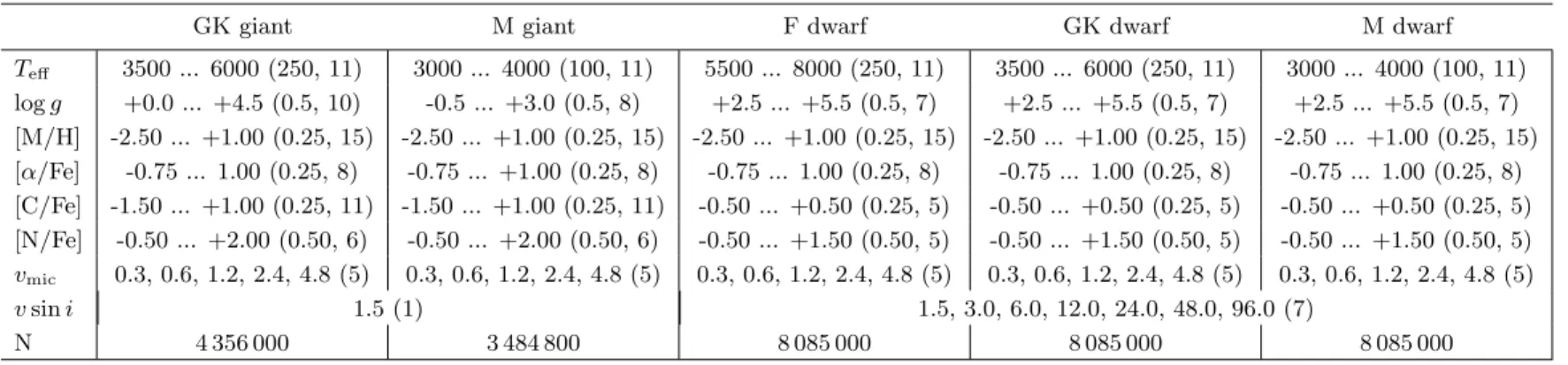
Teff 3500 ... 6000 (250, 11) 3000 ... 4000 (100, 11) 5500 ... 8000 (250, 11) 3500 ... 6000 (250, 11) 3000 ... 4000 (100, 11) logg +0.0 ... +4.5 (0.5, 10) -0.5 ... +3.0 (0.5, 8) +2.5 ... +5.5 (0.5, 7) +2.5 ... +5.5 (0.5, 7) +2.5 ... +5.5 (0.5, 7) [M/H] -2.50 ... +1.00 (0.25, 15) -2.50 ... +1.00 (0.25, 15) -2.50 ... +1.00 (0.25, 15) -2.50 ... +1.00 (0.25, 15) -2.50 ... +1.00 (0.25, 15) [α/Fe] -0.75 ... 1.00 (0.25, 8) -0.75 ... +1.00 (0.25, 8) -0.75 ... 1.00 (0.25, 8) -0.75 ... 1.00 (0.25, 8) -0.75 ... 1.00 (0.25, 8) [C/Fe] -1.50 ... +1.00 (0.25, 11) -1.50 ... +1.00 (0.25, 11) -0.50 ... +0.50 (0.25, 5) -0.50 ... +0.50 (0.25, 5) -0.50 ... +0.50 (0.25, 5) [N/Fe] -0.50 ... +2.00 (0.50, 6) -0.50 ... +2.00 (0.50, 6) -0.50 ... +1.50 (0.50, 5) -0.50 ... +1.50 (0.50, 5) -0.50 ... +1.50 (0.50, 5) vmic 0.3, 0.6, 1.2, 2.4, 4.8 (5) 0.3, 0.6, 1.2, 2.4, 4.8 (5) 0.3, 0.6, 1.2, 2.4, 4.8 (5) 0.3, 0.6, 1.2, 2.4, 4.8 (5) 0.3, 0.6, 1.2, 2.4, 4.8 (5)

vsini 1.5 (1) 1.5, 3.0, 6.0, 12.0, 24.0, 48.0, 96.0 (7)

N 4 356 000 3 484 800 8 085 000 8 085 000 8 085 000

in the flux space of the synthetic spectra (M´esz´aros &

Allende Prieto 2013).

In DR14, the holes in the grid of synthetic spectra were filled by spectral syntheses using the “closest”

neighboring model atmosphere according to a metric specified in Holtzman et al. (2018). This can be extremely inaccurate if the number of holes is significant.

For DR16, we instead implemented radial basis function (RBF) interpolation to fill the missing synthetic spectra in the grids.

The RBF is a real-valued function whose value depends only on the distance from the known points, and works in any number of D dimensions (D ≥ 1) (Buh- mann 2003). The interpolated value is represented as a sum of N radial basis functions (where N is the number of known points). These functions are strictly positive definite functions, and the most widely used definitions are Gaussian, multiquadric, polyharmonic spline, or thin plate spline. We chose the multiquadric form defined below, as it is the most versatile when used with sparse datasets like ours while still achieving the necessary accuracy. Each of the RBF functions are associated with a different known pointxi, weighted by an appropriate coefficientwi, and scaled by the parameterr0:

y(x) =

N

X

i=1

w_i·(||x−x_i||²+r₀²)^0.5

The known points in our case are the synthetic spectra calculated with effective temperature, metallicity, surface gravity, etc., of the converged model atmospheres.

Determining the w_i weights can be accomplished by solving a system of N linear equations, but round-off errors grow large and the required computation time becomes unfeasible long for high values of N, since the computation complexity scales as O(N³).

Therefore, many iterative methods have been developed to reduce the required computation time. One such method is a Krylov subspace algorithm developed by Faul et al. (2005) for multiquadric interpolation in multiple dimensions, which scales as O(N²), a significant improvement compared to direct methods. We implemented this algorithm based on a previous implemen- tation in Matlab available fromGumerov & Duraiswami (2007) who also further optimized Faul et al.’s algorithm by reducing its complexity to O(N*logN). Faul et al.’s algorithm includes two main steps:

1. a precondition phase that depends only on the dis- tances between the known points and a parameter, q, which is the power of the Lagrange functions of the interpolation, and

2. an iteration phase that provides the desired weights for the interpolation.

In the preconditioning phase Faul et al. (2005) care- fully select a set ofqpoints for each known point to con- struct the preconditioner. This preconditioner is used to build a set of directions in the Krylov space for the iteration phase. Largerqvalues will result in fewer iterations (of order∼10 depending on the particular prob- lem), but calculating the preconditioner takes significantly longer. In general cases, when q <<N, a good compromise is to haveqaround 30-50 to limit the computation time of the preconditioner.

In APOGEE’s case we need a different approach.

While the spectra depend on the atmospheric parameters, in a single spectrum the flux only depends on the wavelength, so we do not need to compute the preconditioning phase for every single wavelength. This allows us to save significant computation time by using the same preconditioning for every frequency by selectingq=N. While this increases the complexity of the preconditioning phase, the overall time to determine the weights for

(9)

the entire spectra is reduced significantly, because the choice ofq=N makes the algorithm converge in only 2 or 3 iterations.

A given APOGEE spectral subgrid contains of order 1 000 000 spectra (see Table 2). While the Gumerov

& Duraiswami (2007) algorithm can handle such large number of points in reasonable time, our internal testing showed that the accuracy of how well we can recover missing models degrades significantly when N>2000. It is our goal to be able to recover spectra with 0.01-0.02 or better in normalized flux, an accuracy that is possible to achieve only if we can select 4 or 5 known points in each dimension. For this reason we chose to imple- ment Faul et al.’s method for simplicity and for the fact that it is faster than theGumerov & Duraiswami(2007) approach when N<2000−3000.

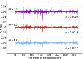
To fill each hole, we use a small grid of models around the hole, where the size of this grid depends on the location in parameter space, but generally has 3-5 points in each dimension. We determine the RBF coefficients for this grid from the filled points and use them to fill the missing point. The shape of the RBF is controlled through the r₀ scale factor, which is recommended to be greater than the minimal distance between points, and significantly less than the maximal distance. It is important to note that no established method exists for determining what is the best scale-factor in terms of accuracy. The best way to evaluate the uncertainties is to temporarily delete known spectra from the grid, re- create them with interpolation, and compare the interpolated spectra with the original ones. After extensive testing of this type, we found thatr0= 1 provided the best accuracy for all grids, except the F-dwarf-subgrid where we chose r0 = 0.5. An example of interpolation errors in one of these tests for three different values of r₀ is shown in Figure3.

The full grids of synthetic spectra are internally labeled “l33” (DR14 used “l31c”), and are available for download from the Science Archive Server⁹. These are available in a series of fits-files, as well as in the FERRE- format described in the code’s manual (see also Allende Prieto et al. 2018).

4.4. Addition of a subgrid for hot stars

For DR16 we added a subgrid suitable for hot stars (Teff>8000 K), thereby analyzing the more featureless spectra of stars that mainly were targeted for removal of telluric lines in the spectra of main survey target stars.

The model atmospheres used for this grid are ATLAS9,

9 https://data.sdss.org/sas/dr16/apogee/spectro/speclib/

synth

Figure 3. Examples of the interpolation error. Of 4096 known spectra in a small subgrid of the larger GK giant grid, 372 were deleted and then re-created using interpolation based on the remaining spectra, using differentr0values, with the aim of evaluating the overall accuracy. Ther0=0.8 and 1.2 cases are shifted up and down in the plot, to aid vis- ibility. On the x-axis are the 372 deleted spectra, and on the y-axis differences between the interpolated and original spectrum forallwavelengths are plotted, i.e. there are thousands of points for every spectrum (x-axis value) and every choice orr0 (0.8, 1.0, 1.2). The statedσis the standard deviation around the mean value. We choser0= 1 because higherr0

values do not improve the accuracy, but add computation time.

the line list is the atomic DR13/14 line list (20150714), and the spectral synthesis code used is Synspec (Hubeny 1988;Hubeny & Lanz 2017). The final subgrid only has four grid dimensions; 7000 K≤Teff≤20 000 K in steps of 500 K (27 steps), 3.0 ≤logg≤ 5 in steps of 0.5 dex (5 steps),−2.5≤[M/H]≤1.0 in steps of 0.5 dex (8 steps), and a projected rotational velocity (vsini) dimension with values of 1.5, 3.0, 6.0, 12.0, 24.0, 48.0, 96.0 km/s (7 steps).

The analysis of these spectra is extremely challenging;

after all, these stars were targeted to show as few spectral features as possible and often hydrogen lines are the only strong features. Still, at least providing an estimate of the basic stellar parameters for these stars might be useful for some science applications. However, it should be noted that these values are not fully evaluated and should be used with caution, preferably by users familiar with hot stars and their spectra.

4.5. Dimensionality reduction using Principal Component Analysis (PCA)

Even after dividing the total number of synthetic spectra into subgrids, these are still too large to hold in memory. Hence we have, as in previous APOGEE data releases, used PCA to reduce the dimensionality of the

(10)

subgrids. Previously, this was done by splitting the APOGEE spectra in 30 pieces and using 30 PCA components for every piece, giving 900 PCA components, which provides almost a factor of 10 reduction in grid size. Tests on synthetic data, comparing the recon- structed spectra to originally calculated spectra, have shown that better accuracy is achieved with the same total number of PCA parameters, but by dividing the spectra in 12 pieces and using 75 PCA components for each piece, so this was implemented for the DR16 grids.

Interpolation is done in the PCA coefficients, and the resulting values are multiplied by the PCA basis functions to create an interpolated spectrum.

4.6. Coarse characterization

In DR14, we did an initial coarse characterization of all stellar spectra to decide which synthetic spectra subgrid(s) to use when performing the stellar parameter determination. This coarse characterization was made by passing all stars through reduced-size F-dwarf, GK- giant, and M-giant grids with [C/M]=[N/M]=0. Based on the outcome of these runs, the spectrum was finally analyzed using the subgrid that yielded the best fit, or two in the case of cases where the best fit was near a grid edge. After the proper subgrid(s) to be used was determined, FERRE was run with 12 different starting positions (to avoid being trapped within local minima) distributed evenly in Teff, logg, and [M/H] in the chosen subgrid(s), and the final stellar parameters were set to the best fitting of these 12 (or 2x12 in the case of border line cases) runs. A more thorough description of this process can be found inHoltzman et al.(2018).

In DR16, we instead created one, large “coarse” grid with dimensions 3000 K≤Teff≤8000 K (11 steps of 500 K), 0≤logg≤5 (6 steps of 1 dex),−2.5≤[M/H]≤

1.0 (8 steps of 0.5 dex), −0.5 ≤[α/M]≤ 1.0 (4 steps of 0.5 dex), −0.5 ≤[C/M]≤ 0.5 (5 steps of 0.25 dex),

−0.5≤[N/M]≤1.0 (4 steps of 0.5 dex), 5 steps ofvmic; 0.3, 0.6, 1.2, 2.4, 4.8 km/s, and 7 steps ofvsini; 1.5, 3.0, 6.0, 12.0, 24.0, 48.0, 96.0 km/s, that was used to decide what “fine” subgrid(s) to use when analyzing the spectrum. Furthermore, the derived values of the stellar parameters from the “coarse” run were adopted as starting values when doing the second “fine” run with FERRE.

This means that in the new scheme, we run FERRE significantly fewer times for every star (1 coarse and 1 or 2 fine), as compared to DR14 (3 coarse and 12 or 24 fine).

This led to a reduction in analysis-time, something that is sorely needed as the data set increases for every release (see Table 1). However, in addition, we changed the choice of minimizing algorithm in FERRE from the default Nelder-Mead algorithm (Nelder & Mead 1965),

identified in the code with the option ALGOR=1, to the Unconstrained Optimization BY Quadratic Approxima- tion or UOBYQA (Powell 2002), ALGOR=3 in FERRE, and this led to a compensatingincreasein analysis time.

Both algorithms perform numerical optimization with- out the need for the explicit evaluation of derivatives, but while Nelder-Mead indicates a prescription for the motion of the vertices of a simplex in the search space that on convergence contains the minimum of the objective function (theχ² in our case), UOBYQA builds quadratic models for minimizing the objective function within trust regions. These changes were motivated by tests analyzing synthetic spectra – that then of course have “known” stellar parameters – which showed that the new scheme produces more accurate results.

4.7. Continuum normalization

For DR16, a revised scheme was used to normalize the spectra. First, the reduction process was improved to provide spectra with smoother variations and less “wig- gles” (see Section 3), helping the normalization of the observed spectra when comparing to the synthetic spectra. In addition, the observed spectra have been slightly continuum-adjusted for the final analysis, based on the fit from the “coarse” fit of stellar parameters. The ratio of the observed spectra to the best-fit “coarse” model spectrum was smoothed with a broad median filter (with a width of 750 pixels) and the observed spectrum was divided by the smoothed residual before being passed to the “fine” run. Manual inspection of spectra and their final, “fine” stellar parameter fits have shown this scheme to greatly improve the continuum fits, and per- haps more importantly, to homogenize the APOGEE-N and APOGEE-S data and decrease the spread in derived stellar parameters/abundances for stars observed with both APOGEE instruments. Finally, both these corrected observed spectra and the synthetic spectra are normalized with a fourth order polynomial in the wavelength region covered by each of the three APOGEE detectors.

For DR16, this final continuum normalization is now made inside FERRE, allowing for rejection of the same pixels (e.g., those contaminated by night sky emission) in the observed and synthetic spectra, based on pixels flagged in the observed spectrum. In previous data releases, the continuum fit of the observed spectrum was made ignoring flagged pixels, while the continuum normalization of the synthetic spectra used all pixels, leading to possible inconsistencies for some spectra.

4.8. Element “windows”

After the stellar parameters (and “abundance parameters”) have been determined, these are held fixed for

(11)

additional runs of FERRE to determine the elemental abundances. For these, only windows in the spectra that are sensitive to the element in question are used, and only the most relevant abundance dimension of the grid is varied; [M/H] (for Na, Al, P, K, V, Cr, Mn, Fe, Co, Ni, Cu, Ge, Rb, Ce, Nd, and Yb), [α/M] (for O, Mg, Si, S, Ca, Ti, and Ti II), [C/M] (for C and C I), or [N/M]

(for N). The windows are chosen based on where our synthetic spectra are sensitive to a given element, and at the same timenotsensitive to another element in the same abundance group. Based on this, different weights are assigned to pixels in different abundance windows, just as in DR14.

In DR16, however, we performed some test analyses using one window at a time for a subset of spectra for the elements with less than 10 windows, with the aim of weeding out windows that produced deviant results for one reason or another, possibly caused by bad/missing atomic data in the window, unrecognized blends, or 3D/NLTE-effects. These analyses were run on a validation sample, which consists of spectra with high S/N, and including stars from across the HR-diagram, stars in the Kepler field, stars with independently determined stellar parameters and abundances, etc.

Based on manual inspection of the derived “window- abundances” as compared to each other, and to expected astrophysical trends in the solar neighborhood, and as a function ofTeff in open clusters, some of the windows used in DR14 were removed for Al, P, S, Ti, V, Cr, Mn, Co, and Yb. The windows and their weights used for DR16 are provided in Table3.

For the elemental abundance determination for DR16, we have used the new TIE option in FERRE for elements that were fit using the [M/H] dimension of the grid.

Using this dimension, abundances of all elements are varied together during the fit. The TIE option allows the [α/M], [C/M], and [N/M] dimensions to be varied oppositely in lockstep, such that the abundances of C, N, and theαelements arenot varied as the best-fitting abundance from the [M/H] variation is determined.

4.9. Other updates

We updated FERRE from version 4.7.1 to the latest version at the time of production, 4.8.5. The updates to the code between these releases are rather minor, but include the important TIE option.

The data were all processed on the SDSS cluster at the University of Utah, which is comprised of 27 nodes with 16 cores each. For processing with FERRE, two jobs are run on each node at once to accommodate the significant memory usage required to load a single subgrid, but the multiprocessing option in FERRE is used

to run 16 threads simultaneously for each job. The total processing time is approximately 8-10 hours per field for fields with a single cohort of∼160 stars.

5. RESULTS

In this section, we describe how the APOGEE DR16 results are presented, and the calibrations that were applied. A subsequent section (Section6) describes some of the validation and attempts to assess accuracy and precision of derived quantities.

The radial velocities, stellar parameters, and abundances for all stars are supplied in a FITS file referred to as the allStar file. For DR16, this file is called allStar- r12-l33.fits¹⁰ (reduction version r12 analyzed with the spectral libraries l33).

5.1. Radial velocities

The radial velocities are provided in the VHE- LIO AVG entry in the allStar file. As in DR14, these velocities are given in the solar system barycentric frame, not the heliocentric frame as the name suggests; the naming convention has been maintained from earlier releases for historical reasons. For stars that have been observed with multiple visits, the scatter of the individu- ally derived radial velocities is provided in VSCATTER.

This can be used, for example, to filter out possible bi- nary systems.

5.2. Stellar parameters

As in previous data releases, and as described in previous sections in this paper, the ASPCAP stellar parameters include the “classic” spectroscopic stellar parameters Teff, logg, [M/H], vmic, and vsini (for dwarfs; a prescribedv_macin the case of giants) as well as some initial estimate of abundances; [α/M], [C/M], and [N/M].

The “abundance parameters” are needed for several reasons; for many of our cool, metal-rich targets, CNO- bearing molecular lines cover more or less the entire APOGEE spectral region and a correct modelling of these is required to fit the classical stellar parameters.

Furthermore, since the α-elements are important elec- tron donors, modelling these correctly as the stellar parameters are determined is necessary, and, additionally, some of our targets have carbon abundances far enough from solar that the atmospheric structure is altered.

These “abundance parameters” are determined from a global fit of the entire spectrum simultaneously with the other stellar parameters.

10 https://data.sdss.org/sas/dr16/apogee/spectro/aspcap/

r12/l33/allStar-r12-l33.fits

(12)

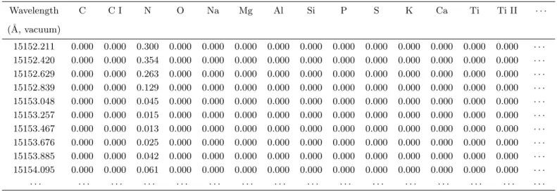
Table 3. Windows and weights used in the determination of stellar abundances. This is only an excerpt of the table to show its form and content. The complete table is available in electronic form.

Wavelength C C I N O Na Mg Al Si P S K Ca Ti Ti II · · ·

(˚A, vacuum)

15152.211 0.000 0.000 0.300 0.000 0.000 0.000 0.000 0.000 0.000 0.000 0.000 0.000 0.000 0.000 · · · 15152.420 0.000 0.000 0.354 0.000 0.000 0.000 0.000 0.000 0.000 0.000 0.000 0.000 0.000 0.000 · · · 15152.629 0.000 0.000 0.263 0.000 0.000 0.000 0.000 0.000 0.000 0.000 0.000 0.000 0.000 0.000 · · · 15152.839 0.000 0.000 0.129 0.000 0.000 0.000 0.000 0.000 0.000 0.000 0.000 0.000 0.000 0.000 · · · 15153.048 0.000 0.000 0.045 0.000 0.000 0.000 0.000 0.000 0.000 0.000 0.000 0.000 0.000 0.000 · · · 15153.257 0.000 0.000 0.015 0.000 0.000 0.000 0.000 0.000 0.000 0.000 0.000 0.000 0.000 0.000 · · · 15153.467 0.000 0.000 0.013 0.000 0.000 0.000 0.000 0.000 0.000 0.000 0.000 0.000 0.000 0.000 · · · 15153.676 0.000 0.000 0.025 0.000 0.000 0.000 0.000 0.000 0.000 0.000 0.000 0.000 0.000 0.000 · · · 15153.885 0.000 0.000 0.042 0.000 0.000 0.000 0.000 0.000 0.000 0.000 0.000 0.000 0.000 0.000 · · · 15154.095 0.000 0.000 0.061 0.000 0.000 0.000 0.000 0.000 0.000 0.000 0.000 0.000 0.000 0.000 · · ·

· · · ·

In the second stellar abundance measurement stage, these abundances are redetermined using windows in the spectra covering only spectral lines sensitive to the abundance in question (see Section5.3). For that reason we recommend the use of these “windowed” abundances in most cases, but even so, the “abundance parameters”

are stored and can be found in the FPARAM-array as well as in the ALPHA M tag.

As in previous data releases, some of the spectroscopically determined stellar parameters have been calibrated to match other, independent measurement of the parameters. These calibrations have varied over the data releases, and we include below a description of what has been done in DR16.

The spectroscopic and calibrated abundance parameters are provided in the FPARAM and PARAM arrays;

there are 9 entries in these arrays for each star, corresponding toT_eff, logg, log(v_mic), [C/M], [N/M], [α/M], log(vsini), and O (currently unused). Many of these are also split out into appropriately named tags in the allStar file, as described below.

5.2.1. Effective temperature,Teff

The spectroscopic T_eff for all stars have been calibrated to the photometric scale ofGonz´alez Hern´andez

& Bonifacio (2009) (GHB) using linear relations as a function of metallicity and effective temperature:

T_eff,cal=T_eff+ 610.81−4.275·[M/H]⁰−

0.116·T_eff⁰ (1) where [M/H] and T_eff are the uncalibrated values of [M/H] and Teff, and the “primed” values are clipped

Figure 4. Difference between spectroscopic DR16 Teff and photometric Teff from Gonz´alez Hern´andez & Bonifacio (2009) as a function of metallicity. Large red and blue points show mean and median differences in bins of metallicity. The adoptedTeff calibration is a function of [M/H] andTeff, and is indicated by the colored lines.

to lie in the range −2.5 <[M/H]⁰ <0.75 and 4500<

T_eff⁰ < 7000. The clipping is applied since the bulk of the stars in GHB fall within these limits, so we prefer not to extrapolate; outside of these ranges, the offsets from the end of the valid range were applied. Figure4 shows the data from which this relation was derived.

The spectroscopically determinedTeffis given in a new TEFF SPEC tag while the calibratedT_eff, as in previous data releases, can be found in the TEFF tag.

5.2.2. Surface gravity,logg

As in DR14, the spectroscopic logg for giant stars have been calibrated using relations determined from stars in the Kepler field for which asteroseismic surface gravities are available (Pinsonneault et al. 2018). As

(13)

with previous data releases, we find that the relationship between the spectroscopic and asteroseismic values is complex; in particular, we find different offsets for red clump and red giant stars that occur in similar locations in aT_eff-logg diagram.

New for DR16 is that we also provide calibrated surface gravities for dwarfs, for which we use a combination of techniques: for warmer dwarfs we have asteroseismic values that we use, while for cooler dwarfs we derive an approximate calibration using isochrones.

The classification of stars into these different “calibration- categories” was done according to the following criteria:

• All stars with uncalibrated logg> 4 or Teff>

6000 K are considered dwarf stars.

• Stars with uncalibrated 2.38<logg<3.5 and [C/N]>0.04−0.46·[M/H]−0.0028·dT are considered red clump stars. HeredTis defined as

dT =Teff,spec− (4400 + 552.6·(loggspec−2.5)−324.6·[M/H]

• RGB-stars are defined as the stars with uncalibrated logg <3.5 andTeff <6000 K that do not fall in the red clump category, as defined above.

• for stars with uncalibrated 3.5 <logg< 4.0 and T_eff< 6000 K, a correction is determined using both the RGB and dwarf calibrations, and a weighted correction is adopted based on logg.

These classifications are shown in Figure 5 in theTeff- loggplane, although this does not show the dependence of the RC/RGB-classification on [M/H] and [C/N].

The calibration relations for dwarf, RC, and RGB stars are respectively:

Dwarf stars:

logg_cal= logg− (−0.947 + 1.886·10⁻⁴·Teff,spec+ 0.410·[M/H]) (2) Red clump stars:

loggcal= logg−

(−4.532 + 3.222·logg−0.528·(logg)²) (3) Red giant stars:

loggcal= logg− (−0.441 + 0.7588·logg⁰−0.2667·(logg⁰)²

+0.02819·(logg⁰)³+ 0.1346·[M/H]⁰) (4)

where

logg⁰ = logg for logg≥1.2795 logg⁰ = 1.2795 for logg <1.2795 [M/H]⁰= [M/H] for [M/H]≤0.5 [M/H]⁰ = 0.5 for [M/H]>0.5

where the fixed value of logg⁰ at low surface gravity and [M/H]⁰ at high metallicity avoids extrapolation into a region where there are few calibrators.

The functional forms for these calibrations were determined from inspection of the relations between spectroscopic, asteroseismic, and isochrone surface gravities.

While these capture a significant portion of the relation- ships, small trends with other parameters may certainly exist, and the calibrated surface gravities cannot be as- sumed to be more accurate than∼0.05 dex.

We note that no smooth transition is implemented between the RGB and RC calibrations resulting in a small discontinuity in loggat the transition value. Based on the asteroseimsic results, we find that 93% of the RGB stars and 96% of the RC stars are classified correctly by our procedure. For the incorrectly classified stars, the calibrated surface gravities will be systematically off. However, since we do the abundance analysis using the uncalibrated parameters, the abundances are unaf- fected.

The spectroscopic logg is given in the LOGG SPEC tag in the allStar file, while the calibrated logg, as in previous data releases, can be found in the LOGG tag.

5.2.3. The abundance parameters; [M/H], [α/M], [C/M], and [N/M]

In DR16, the abundance parameters [C/M], and [N/M] are not calibrated. The [α/M] parameter is calibrated by the application of a zero-point shift of 0.033 dex for giants and 0.01 dex for dwarfs so that the mean of solar metallicity stars in the solar neighborhood has [α/M]=0.0 (see Section 5.3 and Table4).

The [M/H] parameter is also provided in the M H tag, and the calibrated [α/M] parameter is provided in the ALPHA M tag. We note that, due to an inadvertent error, the values in the M H tag (and the corresponding entry in the PARAM array) differ from the values in the FPARAM array by 0.003 and 0.0004 dex for giants and dwarfs, respectively.

5.3. Stellar abundances

In DR16, the abundance determination of 26 species is attempted; C, C I, N, O, Na, Mg, Al, Si, P, S, K, Ca, Ti, Ti II, V, Cr, Mn, Fe, Co, Ni, Cu, Ge, Rb, Ce, Nd, and Yb. Note that, as in previous data releases, the

(14)

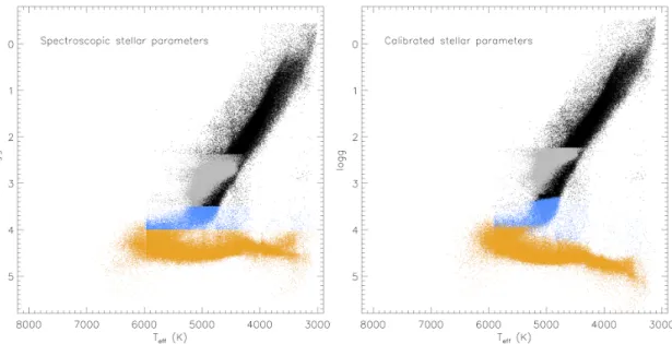
Figure 5. Classification of stars into the logg “calibration-categories”; RGB (black), RC (gray), dwarf (orange), and RGB/dwarf (blue). The left figure shows how the categories were chosen from the spectroscopic stellar parameters, and the right figure shows where the categories end up after calibration. Note in particular the rather sharp RC-RGB “grid edge” at logg∼2.24 in the calibrated parameters. This figure does not demonstrate the dependence of the RC/RGB-classification on [M/H] and [C/N] at a givenTeff and logg.

uncalibrated spectroscopic stellar parameters were used when determining the stellar abundances. The reason for this is that the spectroscopic parameters give the best general fit to the stellar spectrum, and thereby give the best description of possible blends when determining the abundances from the abundance windows.

All of the “raw” abundance measurements for all stars are presented in the FELEM array, in which the order of the array elements for each star is by atomic number, with entries as listed above. Note that, in this array, the abundances for different elements are given with respect to either the total metals or to hydrogen, depending on which grid dimension was used during the fit.

In previous data releases, aTeff-dependent calibration was applied to each individual elemental abundance to remove apparent trends in the uncalibrated abundances, based on observations of star clusters. For DR16 no such calibration is applied because, with the modification to the abundance pipeline, the trends with effective temperature for most elements have reduced amplitude in the cluster sample as compared with previous data processing. That being said, inspection of the full data set suggests that some trends of abundances with stellar parameters can exist for some elements, such that users need to exercise caution when comparing abundances across different regions of stellar parameters space (see Section6.5).

The only calibration applied to the DR16 abundances is a zero-point shift to force stars with solar [M/H] in

the solar neighborhood to have a mean [X/M]=0. This is done separately for giants and dwarfs, where “giants” in this case are defined as stars with logg <

2 + (Tef f −3500)/650 and logg< 4 and Teff<7000 K, and all others are defined as dwarfs. More specifically, we average the “raw” abundances of all stars within 0.5 kpc of the Sun, based on Gaia DR2 parallaxes (Gaia Collaboration et al. 2016,2018; Lindegren et al. 2018), and with−0.05<[M/H]<0.05, and subtract this value from the “raw” [X/M] of all stars. The applied shifts are tabulated in Table4(compare Table 5 inHoltzman et al.

(2018) for the shifts applied in DR13 and DR14); they are generally small (of the order of hundredths of a dex), but are substantial for a handful of elements such as Al, P, V, and Mn. Note that this calibration is a zero-point offset only. Formally, using bracket notation ([X/Fe]) suggests that the abundances are relative to those of the Sun; we did not choose this procedure because many of the lines/elements that we measure in cooler stars are very weak in the solar spectrum, so an APOGEE-based solar abundance measurement has significant uncertainties. Instead, we build upon many results reported in the literature that suggest that the mean [X/Fe] in solar neighborhood stars is close to solar at solar abundance (Reddy et al. 2003;Adibekyan et al. 2012;Bensby et al.

2014, among others). Small intrinsic spread in [X/Fe]

at solar abundance as found byBedell et al.(2018) will still be reflected in the calibrated abundances, as we only apply a single mean offset to all stars.

(15)

The calibrated abundances are provided in the X H and X M arrays in the allStar file, where the difference between these is just the value of M H. For further dis- cussion about the APOGEE abundance scale, see Sec- tion5.3.2.

5.3.1. ”Named” abundance tags, X FE

In addition to the abundances in the X H and X M arrays, we provide abundances in “named” X FE abundance tags, e.g., C FE, N FE, O FE, etc., where we provide abundances relative to iron. These are simply calculated by subtracting the [Fe/H] abundance from the [X/H] abundance for each element.

However, we populate the X FE tags only for stars that we believe the abundances are the most reliable, and do not populate them for abundances that are expected to have large uncertainties or the possibility of significant systematic error. There are a number of reasons why a X FE tag could be unpopulated (i.e., has a value of -9999.99) :

• We do not populate the X FE tags if any bit in the corresponding ELEMFLAG is set. This means that if the estimated uncertainty (see Section5.4) is larger than 0.2 dex, or if the Teff is outside the range in which we think the abundances are reliable (see Section 6.5), then then corresponding X FE tag is not populated.

• For carbon, nitrogen, and iron, the corresponding named tags (C FE, N FE, FE H) are not populated if the elemental window abundance deviates significantly (more than 0.25 dex for C and N, more than 0.1 dex for Fe) from the corresponding “abundance parameter” ([C/M], [N/M], and [M/H]). This behavior is not expected, so these objects are flagged with a PARAM MISMATCH bit in the corresponding ELEMFLAG. Since this can affect FE H, the implication is that none of the named tags (C FE, N FE, O FE, etc.) will be populated for such a star, since the named tags give abundance relative to iron. The bulk of the stars that show this behavior are cool, metal-rich giants, so users are warned that using the named tags will lead to a bias against these stars in a sample. For use cases where such biases may be relevant, users may wish to calculate abundances relative to iron from the X H or X M arrays, recognizing the possibility of some systematic uncertainties for the subset of stars with a PARAM MISMATCH bit set.

• We do not populate the X FE tags for stars with H > 14.6, since for these the RV determination

of the individual visits might fail, leading to bad combination of the spectra, compare Section6.2.

• We do not populate the CE FE tag for stars with vrad>120, because for these stars, the window for the single Ce line that is used shifts into wave- lengths that fall in one of the gaps between the APOGEE detectors.

• We do not populate the named tags for several un- reliable elements, includingall abundances of Ge, Rb, and Yb because the few lines available are so weak/blended that we cannot determine these abundances reliably¹¹. The Nd abundances are also completely removed in the ND FE tag, but in this case the reason is mainly limitations in the current methodology; the available Nd lines are all blended with lines that also vary in the [M/H] dimension, which means that we cannot distinguish the Nd-contribution to the absorption line from the contribution from the blending element. The abundances for these four elements were also removed in the named tags in DR14.

As a result of these criteria, users should be aware that using abundances from the named tags will yield a sample with additional biases over those present from selection effects, in exchange for getting a sample with abundances that are expected to be more reliable. The abundances in the X M and X H arrays are not subject to these additional biases, but may be less reliable for some stars.

5.3.2. The abundance scale

The solar abundance scale of DR16 is complex, but, in general, we are likely to be close to the scale ofGrevesse et al. (2007) for many elements. The relevant steps in making this a hard question are re-iterated below:

• When constructing the line list for the analysis, we adjust the atomic data to fit a spectrum of the Sun with the Grevesse et al. (2007) abundances (and the parameters T_eff=5777 K, logg=4.44, [Fe/H]=0.00, vmic=1.10 km/s), but only within the quoted uncertainties of the source of the data. Moreover, we simultaneously adjust the atomic data to also fit a spectrum of Arcturus (with the parameters Teff=4286 K, logg=1.66, [Fe/H]=-0.52, v_mic=1.74 km/s), and abundances

11 In addition to the Rb line being very weak, an incorrect wavelength of 15289.966 ˚A (air) from the Kurucz line list was used when constructing the spectral grids, instead of the correct 15289.480 ˚A(air), rendering the Rb abundances in DR16 useless.

(16)

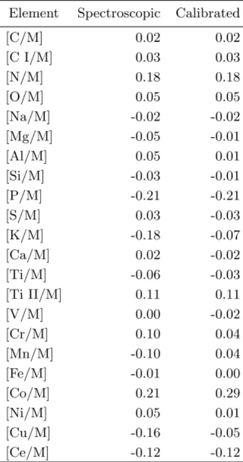
Table 4. The determined abundances are zero-point shifted to make stars with solar M H in the solar neighborhood have [X/M]=0. Below is the list of the applied shifts for giant and dwarf stars, respectively. For Na, P, Ti II, and Ce no calibrated abundances are given for dwarfs because of large uncertainties, see Section 6.10.

Element Giants Dwarfs [C/M] 0.000 +0.003 [C I/M] 0.000 -0.003 [N/M] 0.000 +0.002 [O/M] -0.022 -0.001 [Na/M] -0.022 · · · [Mg/M] -0.009 +0.041 [Al/M] -0.148 -0.043 [Si/M] -0.038 +0.026 [P/M] +0.183 · · · [S/M] -0.040 -0.054 [K/M] +0.090 +0.108 [Ca/M] -0.002 -0.035 [Ti/M] -0.009 +0.027 [Ti II/M] -0.249 · · · [V/M] +0.192 -0.026 [Cr/M] +0.020 -0.065 [Mn/M] +0.121 +0.145 [Fe/M] 0.000 0.000 [Co/M] -0.027 +0.079 [Ni/M] -0.016 -0.043 [Cu/M] +0.018 +0.103 [Ce/M] -0.070 · · · [M/H] 0.000 +0.003 [α/M] -0.033 -0.011

from the literature (see Smith et al. in prep for details). Molecular data are not adjusted.

• The chemical abundances in the stellar atmosphere models and the spectral synthesis calculations are specified relative to the solar abundance scale ofGrevesse et al.(2007).

• The calibrated abundances have been zero-point corrected so that solar-metallicity stars in the solar neighborhood have [X/M]=0; see Table4. We do not calibrate directly to the Sun because it is not

typical of the stars in the APOGEE sample, and because abundances of many elements are not well determined in stars with effective temperature as high as that of the Sun. Note, however, that the calibration offsets are small for many elements, as shown in Table4. C and N abundances have not been calibrated for giants since those abundances are expected to be affected by the star’s evolution and not follow Galactic chemical evolution.

We stress that the uncalibrated abundances derived for giants from molecular lines – C, N, O – are not adjusted in any way and, provided the molecular data do not have systematic uncertainties, those abundances should be at least close to the Grevesse et al. (2007) scale. Regarding the uncalibrated abundances derived from atomic lines, the abundance scale varies from element to element. For elements that have strong features in the Sun, the adjustments to the atomic data do not depend much on the fitting of the Arcturus spectrum/abundances, and if these same features happen to have high weight in the ASPCAP analysis, the abundance scale should be close to that of Grevesse et al.

(2007). For elements whose abundance determination rely more on lines whose loggf-values were more adjusted using the Arcturus spectrum, the absolute abundance scale is less well known. The fact that the adjustments to the atomic data depend on Arcturus as well as the Sun is a significant motivation for calibrating the derived spectroscopic stellar abundances based on the solar neighborhood solar metallicity stars. C and N in giants do not have any calibration applied and should – if we assume that the molecular data used does not have any systematics – be at least close to theGrevesse et al.

(2007) scale. For all other calibrated abundances our philosophy is that they are provided on a “true bracket”

(i.e., relative) scale in the spectroscopic sense, where abundances are simply presented in a ratio to our own, undetermined, unspecified solar abundance.

A check on our solar reference scale is provided by our analysis of the solar spectrum reflected off the asteroid Vesta (see Table5). However, we stress again that the Sun is not a typical star within the APOGEE sample, and that these values cannot be taken as deviations from theGrevesse et al. (2007) scale for the main sample of APOGEE.

5.4. Uncertainties

As in DR14, we find that the uncertainties for parameters and abundances returned by the fitting routine in FERRE are unrealistically low in most cases. As a result, we take an alternate approach to derive empiri- cal uncertainties, and adopt for the final uncertainties