A new method to simulate restricted variants of polarizationless P systems with active

(1)

A new method to simulate restricted variants of polarizationless P systems with active

membranes

Zsolt Gazdag^1? and G´abor Kolonits^2??

1 Department of Foundations of Computer Science University of Szeged

gazdag@inf.u-szeged.hu

2 Department of Algorithms and their Applications Eötvös Loránd University

kolomax@inf.elte.hu

Abstract. According to theP conjectureby Gh. P˘aun, polarizationless P systems with active membranes cannot solveNP-complete problems in polynomial time. The conjecture is proved only in special cases yet.

In this paper we consider the case where only elementary membrane division and dissolution rules are used and the initial membrane structure consists of one elementary membrane besides the skin membrane. We give a new approach based on the concept of object division polynomials introduced in this paper to simulate certain computations of these P systems. Moreover, we show how to compute efficiently the result of these computations using these polynomials.

Keywords: Membrane Computing, active membranes, computational complexity

1 Introduction

P systems with active membranes, introduced in [13], are among the most investigated variants of P systems. Using the polarizations of the membranes and the possibility of dividing elementary (or even non-elementary) membranes these systems can solve computationally hard problems efficiently. More precisely, with elementary membrane division they can solveNP-complete problems [8,13,17,20], while with non-elementary membrane division they can solve even PSPACE- complete problems efficiently [1,18]. Solving computationally hard problems with P systems with active membranes has a huge literature in Membrane Computing, see e.g. [2,5,6,10,12,16], and the references therein.

?Research of this author was supported by the Ministry of Human Capacities, Hun- gary, grant no. 20391-3/2018/FEKUSTRAT.

?? Research of this author was supported by NKFIH – National Research, Development, and Innovation Office, Hungary, grant no. K 120558.

(2)

It is a frequently investigated question whether these P systems are still powerful enough to solve hard problems when the polarizations of the membranes are not used (see e.g. [3,7,9,11,19]). In the case when non-elementary membrane division is allowed the answer to this question is positive since in [3] thePSPACE-complete QSAT problem was solved efficiently without polarizations. On the other hand, no efficient solutions of hard problems exist when non-elementary membrane division is not allowed. In fact, Gh. P˘aun conjec- tured already in 2005 that without polarization and non-elementary membrane division P systems with active membranes cannot solveNP-complete problems in polynomial time [14]. P˘aun’s conjecture, often called the P conjecture, has not been proven yet. A direct attempt to calculate efficiently all the elementary membranes of a computation of such a P system fails as in general the number of these membranes is exponential and, moreover, these membranes can contain pairwise different multisets. However, it was discovered in [7] that if dissolution rules are not allowed to use, then there is no need to simulate all the elementary membranes to determine the result of a computation. Instead, it is enough to consider a certain graph, called the dependency graph [4] of the P system.

Roughly, this graph describes how the rules of the P system can evolve and move objects through the membranes. To determine the result of a computation in this case it is enough to check whether a distinguished object is reachable from certain objects in the dependency graph.

If dissolution rules are also allowed, then things became much more compli- cated. Consider a P systemΠ with active membranes and assume, for example, that Π contains a membrane sub-structure [[a b]₂]₁. Assume moreover that a can dissolve membrane 2 but b cannot. ThenΠ dissolves membrane 2 using a, and b immediately gets to membrane 1 without directly being involved in any application of a rule. Notice that when b gets to membrane 2 then it “knows”

that Π contained an occurrence of ain the same membrane. This way the objects can send information to each other and this kind of behaviour cannot be captured by dependency graphs.

Using generalizations of dependency graphs the P conjecture was already proved in some special cases where the P systems were allowed to use dissolution rules as well. In [19], for example, the P conjecture was proved usingobject division graphs in the case where the initial membrane structure of the P system is a linearly nested sequence of membranes, and the system can employ only dissolution and elementary membrane division rules. In [9] the P conjecture was proved in another case using a generalization of dependency graphs.

Here the P systems are deterministic, can use all types of rules except send-in communication rules, and the membrane structure is such that the skin contains only elementary membranes. In these papers the authors used these generalizations of dependency graphs in order to simulate a reasonable small part of the configurations in a computation of the investigated P systems.

In this paper we propose a new method for simulating polarizationless P systems using both division and dissolution rules. Using this method it is possible to calculate efficiently the number of objects appearing in the skin membrane

(3)

during a computation of a P system. Our approach can be roughly described as follows. Consider a P system Π, its input multisetω, and a computation C of Π. First we define object division polynomials based on the concept of object division graphs. The object division polynomial of an object adescribes which and how many objects can be created by Π using only division rules starting the division usinga. Then we consider a polynomial Pω which is, roughly, the multiplication of the object division polynomials of objects inω. We show that there is a strong relationship between the monomials of Pω and the number of certain membranes in C. Using this we can calculate efficiently which and how many objects get to the skin membrane in each step ofC.

In order to make the presentations as transparent as possible, we give our method only for a rather restricted variant of P systems. In this variant the P systems, for example, have only one elementary membrane in the skin at the beginning of the computation and can employ only membrane division and membrane dissolution rules. Moreover, we will simulate only such computations of these P systems, where division rules have priority over dissolution rules.

However, we believe that our method can be extended to more general variants of P systems as it is discussed in the Conclusions section.

2 Preliminaries

Here we recall the necessary notions used later. Nevertheless, we assume that the reader is familiar with the basic concepts of membrane computing techniques (for a comprehensive guide see e.g. [15]).

N denotes the set of natural numbers and, for every i, j ∈ N, i ≤ j, [i, j]

denotes the set {i, i+ 1, . . . , j}. If i = 1, then [i, j] is denoted by [j]. We will use polynomials with coefficients inN. A polynomial of the formp=cx^j₁¹. . . x^j_nⁿ wherec, n∈N, x1, . . . , xn are variables, andj1, . . . , jn≥1 is called a monomial and c is called the coefficient of p. An n×m matrix M has n rows and m columns. We will consider matrices with entries in N. (M)ij denotes the jth element of theith row ofM. By avector vwe mean ann×1 matrix, for some n≥1.v^T denotes the transpose ofv, and instead of (v)j1 and (v^T)1j (j ∈[n]) we will write simply (v)j and (v^T)j, respectively. If a vectorvhasnentries, for some n≥1, thenvis called an n-dimensional vector or just ann-vector.

In this paper we consider polarizationless P systems. A polarizationlessP system with active membranes [13] is a construct of the form Π = (O, H, µ, w₁, . . . , w_m, R), where m is the initial degree of the system, O is the alphabet of objects, H is the set oflabels of the membranes, µ is a membrane structure consisting of mmembranes labelled with the elements ofH in a one- to-one manner,w₁, . . . , w_m∈O^∗are theinitial multisets of objects placed in the mregions ofµ; andR is a finite set ofrules defined as follows:

(a) [a→v]h, whereh∈H, a∈O, v∈O^∗ (objectevolution rules);

(b) a[ ]h→[b]h, whereh∈H,a, b∈O (send-in communication rules);

(4)

(c) [a]_h→[ ]_hb, whereh∈H,a, b∈O (send-out communication rules);

(d) [a]_h→b, where,h∈H,a, b∈O (membrane dissolution rules);

(e) [a]_h→[b]_h[c]_h, whereh∈H,a, b, c∈O (division rules for elementary membranes).

For any rulerof the formu→v,u(resp.v) is called theleft-hand side(resp.

theright-hand side) ofr.

As it is usual in membrane computing, P systems with active membranes work in a maximally parallel manner: at each step the system first nondeter- ministically assigns appropriate rules to the objects of the system such that the assigned multiset S of rules satisfies the following properties: (i) at most one rule fromS is assigned to any object of the system, (ii) a membrane can be the subject of at most one rule in S, and (iii)S is maximal among the multisets of rules satisfying (i) and (ii).

LetΠ = (O, H, µ, w1, . . . , wm, R) be a polarizationless P system with active membranes. Π is called a simple divide-dissolve P system (sdd P system, for short) if

– H={1, s}andµ= [[ ]1]s,

– Π employs only membrane division and membrane dissolution rules, – different rules ofΠ have different left-hand sides, and

– the dissolution rules have the form [a]1→a(a∈O).

We call a membrane with label 1 a working membrane (notice that as the skin cannot be divided or dissolved, the objects in the skin are not changing as they cannot evolve in any way). An object a∈ O is called a divider ifacan divide working membranes, that is,Rcontains a division rule with [a]1on the left-hand side. Likewise, an object a ∈ O is called a dissolver if a can dissolve working membranes, that is, R contains the dissolution rule [a]₁ → a. Furthermore,Π is called halting, if each of its computations halts. In the rest of the paper we consider only polarizationless halting sdd P systems.

3 Results

In the rest of the paper let Π = (O,{s,1},[[ ]1]s, ω1, ωs, R) be a halting sdd P system, whereO ={a1, . . . , a_n} (n∈N) and ω₁=a_i₁. . . a_i_m, for somem ≥1 andi₁, . . . , i_m∈[n]. To simplify the arguments we assume also thatω_s=ε.

In this section we show that the multiset content of the skin membrane of Π at the end of the so-called division driven computations can be computed in polynomial time in nm. In division driven computations division rules have priority over dissolution rules and there is a certain order between the division rules too. To specify these computations precisely we need some preparation.

Consider a halting computation C : C0 ⇒ C1 ⇒ . . . ⇒ Ct of Π. We first assign to each occurrence of an object occurring in a working membrane a label

(5)

defined inductively as follows. The label of an objecta_i_` (`∈[m]) inω₁ inC₀ is

`. Now, letM be a working membrane inC_i, for somei∈[0, t−1], and consider an occurrence of an objectainM with label`(`∈[m]). Then we have exactly one of the following three cases: (i) this occurrence of a is not involved in the application of any rule, or (ii) it is involved in the application of a division rule r : [a]1 →[b]1[c]1, or (iii) it is involved in the application of a dissolution rule during Ci ⇒ Ci+1. In Case (i) the same occurrence of a occurs in Ci+1 too.

Then let the label of this occurrence ofainCi+1 be`. In Case (ii)r dividesM into two new membranes inCi+1. Then let the label of the occurrences ofband cintroduced byrin these two new membranes be`. In Case (iii) no objects are introduced in the working membranes by the considered occurrence of a, thus no labelling is necessary in this case. Ifais an object with label`, then we will often denote this bya^(`).

Notice that the multiset content of a working membrane inCalways has the form a⁽¹⁾_j

1 . . . a^(m)_j

m , for some j₁, . . . , j_m ∈[n]. Using the labels of the objects we can define now division driven computations as follows.

Definition 1. Consider a halting computation C.C is called division driven if when a division rule is applied in a membrane M triggered by an object a^(`)_i (i∈[n], `∈[m]), then M contains no objecta^(`

0)

j with `⁰ < ` such that aj can divide M.

Intuitively, in a division driven computationC ofΠ the computation goes as follows. Assume that the labels of those objects in ω₁ that can divide working membranes are `₁ < . . . < `_k, for some k ∈[m]. Then first objects with label

`₁ are used to divide working membranes, then those objects which have label

`₂, and so on until at the end those objects are used which have label`_k. Then those objects are used which can dissolve working membranes, and if no more working membranes can be dissolved, the computation terminates. Notice that if a non-dividing objectawith label`occurs in a working membrane, then this object remains unchanged until the computation halts.

Example 1. LetΠex= ({a1, a2, a3, a4},{s,1},[[ ]1]s, a⁽¹⁾₁ a⁽²⁾₁ , ε, R), where R={[a1]1→[a2]1[a3]1,[a2]1→[a4]1[a4]1,[a4]1→a4}.

Figure 1 shows a division driven computation ofΠex. Recall that the numbers in parentheses are the labels of the corresponding objects. Notice that each working membrane contains two objects with labels 1 and 2, respectively. ut Now we define a concept similar to that ofobject division graphs (see e.g. in [19]). The object division tree of a_i (i ∈ [n]), denoted by odt_a_i is the smallest binary tree satisfying the following conditions:

– the root of odtai is labelled byai, and

– if a nodeN of odt_a_i is labelled by a_j (j ∈ [n]) and [a_j]₁ → [a_k]₁[a_l]₁ ∈R (k, l ∈[n]) then N has exactly two children with labels ak and al, respectively.

(6)

Fig. 1.A division driven computation ofΠexfrom Example 1. Grey areas are regions of working membranes.

Since Π is an sdd P system, it does not have different division rules with the same left-hand side. Thus odta_i is well defined. Notice that in odta_i a subtree with a root labelled by an object aj (j ∈ [n]) is equal to odta_j. The height of odtai, denoted byh(odtai), is defined inductively as follows. If odtai is a single node labelled by a_i, then h(odt_a_i) = 0. Otherwise leth_max be the maximum of the heights of subtrees of the root in odt_a_i. Thenh(odt_a_i) =h_max+ 1.

Example 2. Consider againΠex from Example 1. The tree odta₁ can be seen in Figure 2. Notice that odta₂ and odta₃ are equal to the first and second subtrees of odta₁, respectively, and odta₄ is equal, for example, to the first subtree of

odta₂. ut

Fig. 2.The tree odta₁ from Example 2.

Next we show a useful property of object division trees.

(7)

Lemma 1. ConsiderΠ andi∈[n] such thata_i occurs inω₁. Then h(odt_a_i)<

n.

Proof. We give an indirect proof. Assume thath(odta_i)≥n. Then there exists a pathP in odta_i with length at least n. Due to the pigeonhole principle, there exists j ∈ [n] such that aj occurs at least twice in P. Let N1 and N2 be the first two nodes of P (counted from the root) labelled by aj. Let t1 and t2 be the subtrees of odt_a_i with roots N₁ and N₂, respectively. Clearly, t₂ is a proper subtree of t₁. Moreover, by our above note t₁ =t₂ = odt_a_j. This implies that odt_a_i is infinite, which further implies that a division driven computation will never halt. However, this contradicts to the fact thatΠ is a halting sdd P system,

proving our statement. ut

Notice that, for every division driven halting computationC:C0⇒C1⇒. . .⇒ CtofΠ,t≤ P

ai∈ω1

h(odta_i) + 1.

Every object division tree defines anobject division polynomial as follows.

Definition 2. ConsiderΠ and letV ={xi|i∈[n]} ∪ {x} be a set of variables.

Let moreover i ∈ [n] and l = h(odti). The object division polynomial of ai

(odp_a_i for short) is a polynomial with variables inV defined as follows:

odp_a

i= X

j∈[0,l],k∈[n]

m_jk·x_k·x^j,

wheremjk is the number of leaves in odta_i at depthj labelled by ak.

Example 3. Consider Π_ex from Example 1 and the object division trees considered in Example 2. The corresponding object division polynomials are as follows:

– odp_a₁= 2x4x²+x3x, – odp_a

2= 2x₄x, – odp_a₃=x3, – odp_a

4=x₄.

u t

Next we show that object division polynomials can be calculated efficiently.

Lemma 2. ConsiderΠ and leti∈[n]. Thenodp_a

i can be computed in polynomial time inn.

Proof. Let l=h(odta_i)and, for every j∈[0, l], letvj be ann-vector such that (vj)k (k ∈ [n]) is the number of nodes labelled by ak on the jth level of odtai. Let ndiv={j∈[n]|a_j is a non-divider}. As the set of labels of leaves in odt_a_i is included in the set{aj |j∈ndiv}, we get that

odp_a_i = X

j∈[0,l],k∈[n]

vjekxkx^j,

(8)

wheree_k (k∈[n]) is ann-vector defined as follows:

(ek)s=

(1 if s=k andk∈ndiv 0 otherwise.

To compute v_j (j ∈ [0, l]) let us define, for every k ∈[n], the n-vector m_k as follows: for every s∈[n], if there is a ruler with a_s on the left- anda_k on the right-hand side, then let(mk)sbe the number of occurrences of ak on the right- hand side ofr. If there is no such rule inR, then let(mk)sbe0. It can be clearly seen that if we multiplyv_j^T (j∈[0, l−1]) withmk (k∈[n]), we get the number of occurrences ofak on the(j + 1)th level ofodta_i. Thus, for every j∈[0, l−1], v^T_j+1=v_j^TM, where M is then×nmatrix whose kth column (k∈[n])is mk. Since matrix multiplication is associative, we get thatv^T_j =v^T₀M^j (j∈[l]). This implies that

odp_a_i = X

j∈[0,l],k∈[n]

v₀^TM^jekxkx^j.

Notice that since the0th level ofodtai contains only the root ofodtai,(v0)k = 1 if k=i, and(v₀)_k= 0 otherwise. Therefore, the coefficient of a factorx_kx^j in odp_a

i is (M^j)_ik. Thus, we only have to compute M^j for every j ∈[0, l]. Since every row in M contains at most two non-zero elements and the sum of these elements is two, it is easy to see that the largest value inM^j is at most2^j. So these values can be stored usingnbits and thus computing one entry ofM^j+1can be done in O(n)steps. Since M is ann×n matrix, computing every necessary

value can be done in polynomial time inn. ut

Example 4. Consider odp_a₁ and odp_a₂ given in Example 3. According to the proof of Lemma 2, we can compute these polynomials as follows. We will useei

(i∈[4]) andM^j (j∈[0,2]) in the computation of each polynomial. These have the following values:e^T₁ =e^T₂ =

0 0 0 0

,e^T₃ = 0 0 1 0

,e^T₄ = 0 0 0 1

,and

M⁰=





 1 0 0 0 0 1 0 0 0 0 1 0 0 0 0 1





 ,M¹=





 0 1 1 0 0 0 0 2 0 0 0 0 0 0 0 0





 ,M²=





 0 0 0 2 0 0 0 0 0 0 0 0 0 0 0 0





 .

Moreover, in the case of odp_a₁ v₀^T = [1 0 0 0] andl= 2. Clearly, X

j∈[0,2],k∈[4]

v^T₀M^jekxkx^j= X

k∈[4]

v^T₀M⁰e_kx_k+ X

k∈[4]

v^T₀M¹e_kx_kx+ X

k∈[4]

v^T₀M²e_kx_kx².

(9)

Thus, in the case of odp_a

1 we get that X

j∈[0,2],k∈[4]

v^T₀M^jekxkx^j= X

k∈[4]

[1 0 0 0]e_kx_k+ X

k∈[4]

[0 1 1 0]e_kx_kx+

X

k∈[4]

[0 0 0 2]ekxkx²= (0x1+ 0x2+ 0x3+ 0x4)+

(0x1x+ 0x2x+ 1x3x+ 0x4x) + (0x1x²+ 0x2x²+ 0x3x²+ 2x4x²) = 2x₄x²+x₃x= odp_a

1.

On the other hand, in the case of odp_a₂ v^T₀ = [0 1 0 0] andl= 1. Thus we get the following calculation.

X

j∈[0,1],k∈[4]

v^T₀M^je_kx_kx^j = X

k∈[4]

[0 1 0 0]ekxk+ X

k∈[4]

[0 0 0 2]ekxkx=

(0x1+ 0x2+ 0x3+ 0x4) + (0x1x+ 0x2x+ 0x3x+ 2x4x) = 2x₄x= odp_a

2.

u t Object division polynomials can be used to calculate the multiset contents of certain working membranes occurring in a division driven computation ofΠ. To see this we need some preparation. First we extend the definition of object division polynomials to objects having labels.

Definition 3. Consider Π and letodp_a_i = P

j∈[0,l],k∈[n]

mjkxkx^j. Let moreover

`∈[m]. The labelled object division polynomial of a^(`)_i ( lodp_a(`) i

for short) is the polynomial P

j∈[0,l],k∈[n]

mjkx`kx^j (that is, we add`to the indices of variables of odp_a

i, referring this way to the label of the corresponding object).

Consider a division driven computation C:C₀⇒C₁ ⇒. . .⇒C_t of Π. Let M be a working membrane inCand`∈[m]. IfM contains no dividers with label

`⁰ ≤ `, then M is called `-divider-stable. Moreover, m-divider-stable working membranes are called non-dividing. Consider an `-divider-stable membrane M in C_i (` ∈ [m], i ∈ [t]). M is called primary if either i = 0 or the following holds. Let N be that membrane inC_i−1 from which Π derives M. Then N is not`-divider-stable.

Example 5. LetΠexbe the P system given in Example 1 and consider the working membrane M containing a⁽¹⁾₃ a⁽²⁾₂ in C2. ThenM is 1-divider-stable, as the

(10)

only object in M having label 1 or less isa₃ which is a non-divider. However, this M is not 2-divider-stable, since it contains a₂ having label 2 and a₂ is a divider. M is neither primary, asM is derived from the working membrane N in C₁ containinga⁽¹⁾₃ a⁽²⁾₁ butN is 1-divider-stable, too. However,N is primary, since it is derived from the working membrane in C₀ containinga⁽¹⁾₁ a⁽²⁾₂ , which is not 1-divider-stable.

The only working membrane inC₅ is non-dividing, as it is 2-divider-stable, and 2 is the greatest label in this example. Notice that non-dividing working membranes are those which do not contain dividers. ut Next we define a product of labelled object division polynomials ofΠ which we will use frequently in what follows.

Definition 4. Consider again Π and its initial membrane content ω₁. The ω₁- product ofΠ isP_ω₁ = Q

`∈[m]

lodp_a(`) i`

.

It is easy to see that all monomials in P_ω₁ have the form αx_1j₁. . . x_mj_mx^j, for some α, j ∈Nand j₁, . . . , j_m∈[n]. In the next lemma we show that there is a strong relationship between the monomials inP_ω₁ and the primary non-dividing working membranes of a division driven halting computation of Π.

Lemma 3. ConsiderΠ, itsω₁-productP_ω₁, and a division driven halting computation C : C₀ ⇒ C₁ ⇒ . . . ⇒ C_t of Π. Let moreover j₁, . . . , j_m ∈ [n] and j ∈ [0, t]. Then the coefficient of x_1j₁. . . x_mj_mx^j in P_ω₁ equals to the number of those primary m-divider-stable working membranes in Cj which contain a⁽¹⁾_j

1 . . . a^(m)_j

m .

Proof. We show the statement by induction on m. If m = 0, then Pω₁ is the empty product, that is, Pω1 = 1. In this case Pω1 can be considered as the monomial x⁰, where the coefficient is one. On the other hand, C consists of C₀ only. C₀ has exactly one working membrane, which is empty and primary m-divider-stable. This proves the statement in this case.

Now assume that the statement holds ifm=m⁰, for somem⁰≥0. We show it for m = m⁰ + 1. Let α be the coefficient of a monomial x_1j₁. . . x_mj_mx^j in P_ω₁. Let moreover ˆαbe the number of those primarym-divider-stable working membranes inCj which contain a⁽¹⁾_j

1 . . . a^(m)_j

m . We show thatα= ˆα.

Letω₁⁰ =ai₁. . . ai_m0 and P_ω⁰

1 = Q

`∈[m⁰]

lodp_a(`) i`

. Clearly, Pω₁ =P_ω⁰

1lodp_a(m) im

. Let us denote byαj⁰ andβj⁰⁰ (j⁰, j⁰⁰∈[t]) the coefficients ofx1j₁. . . xm⁰j_m0x^j⁰ in P_ω⁰

1 andx_mj_mx^j⁰⁰ in lodp_a(m) im

, respectively. One can see thatαcan be calculated by summing up the productsαj⁰βj⁰⁰, for everyj⁰, j⁰⁰∈[t] withj⁰+j⁰⁰=j.

On the other hand, letj⁰, j⁰⁰ ∈[t] and denote ˆαj⁰ the number of those primary m⁰-divider-stable working membranes in Cj⁰ which contain a⁽¹⁾_j

1 . . . a^(m

0) j_m0 . Denote, moreover, ˆβj⁰⁰ the number of leaves labelled byaj_m in odta_im at depth j⁰⁰. Consider now a membraneM inCjcontaininga⁽¹⁾_j

1 . . . a^(m)_j

m . One can see that

(11)

the only way for Π to create M is the following. First Π creates a membrane N containinga⁽¹⁾_j

1 . . . a^(m_j ⁰⁾

m0 a^(m)_i

m in j⁰ steps (j⁰ ∈[t]) using only dividers having labelsm⁰ or less. Then, using dividers with labelm,Π createsM inj⁰⁰=j−j⁰ steps. Thus ˆαcan be calculated by summing up the products ˆαj⁰βˆj⁰⁰, for every j⁰, j⁰⁰∈[t] with j⁰+j⁰⁰=j.

By induction hypothesis, α_j⁰ = ˆα_j⁰, for every j⁰ ∈ [t]. Moreover, by the definition of object division polynomials,β_j⁰⁰= ˆβ_j⁰⁰, for everyj⁰⁰∈[t]. Thus we have that

α= X

j⁰,j⁰⁰∈[t], j⁰+j⁰⁰=j

α_j⁰β_j⁰⁰= X

j⁰,j⁰⁰∈[t], j⁰+j⁰⁰=j

ˆ

α_j⁰βˆ_j⁰⁰= ˆα,

which finishes the proof of the lemma. ut

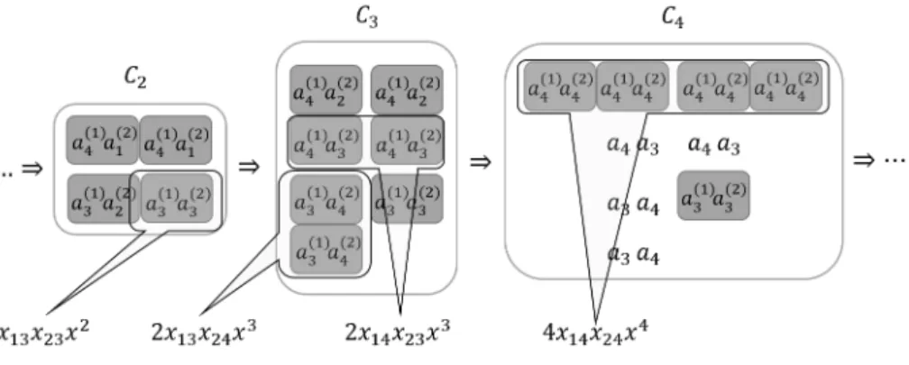
We show now through an example how to usePω₁ to calculate multiset contents of certain membranes.

Example 6. Consider Πex from Example 1 and the computationC given in Fig- ure 1. From Example 3 we know that odp_a₁ = 2x4x²+x3x. Thus lodp_a(1)

1

= 2x14x²+x13xand lodp_a(2)

1

= 2x24x²+x23x. AsP_a(1)

1 a⁽²⁾₁ = lodp_a(1) 1

lodp_a(2) 1

we get that

P_a(1)

1 a⁽²⁾₁ = (2x₁₄x²+x₁₃x)(2x₂₄x²+x₂₃x) =

4x₁₄x₂₄x⁴+ 2x₁₄x₂₃x³+ 2x₁₃x₂₄x³+x₁₃x₂₃x². Figure 3 shows the correspondence between the monomials of P

a⁽¹⁾₁ a⁽²⁾₁ and the primary non-dividing working membranes ofC. Notice that the variablesx_ij (i∈ [2], j∈[4]) correspond to objectsa⁽ⁱ⁾_j , the coefficient of a monomial corresponds to the number of the corresponding membranes, and the power of xshows the

index of the corresponding configuration. ut

Consider againΠ and a division driven halting computationC of Π. As we have seen, the multiset content of the primary non-dividing working membranes ofCcan be calculated by determining the monomials ofP_ω₁. Clearly, if we know these multisets, then we can tell which and how many objects are sent to the skin (by applying membrane dissolution rules) in each step of C. However, the size ofPω₁ can be exponential innm, which means that we cannot usePω₁ directly to calculate the number of these objects efficiently. Instead, we will use another polynomial given by using the following definition.

Definition 5. Consider Π and let P be a polynomial over the variables V = ({x`k|`∈[m], k∈[n]} ∪ {x}). Let moreoveri∈[n]andybe a new variable not occurring in V. The i-reduction ofP is the polynomial P^hii which we get from P by performing the following operations. First, for every`∈[m], k ∈[n] with

(12)

Fig. 3.The representation of non-dividing working membranes ofΠexby monomials.

k6=i, let us substitute x`k inP with z, where

z=

(y, if a^(`)_k can dissolve working membranes, and 1, otherwise.

Let the given new polynomial beP⁰. Then letP^hiibe the polynomial created from P⁰ by substituting x_`i withx_i, for every `∈[m].

Example 7. The i-reductions (i ∈ [4]) of P_a(1)

1 a⁽²⁾₁ given in Example 6 are as follows:

P^h1i

a⁽¹⁾₁ a⁽²⁾₁ = 4yyx⁴+ 2y1x³+ 2·1yx³+ 1·1x²= 4y²x⁴+ 4yx³+x² P^h2i

a⁽¹⁾₁ a⁽²⁾₁ = 4yyx⁴+ 2y1x³+ 2·1yx³+ 1·1x²= 4y²x⁴+ 4yx³+x² P^h3i

a⁽¹⁾₁ a⁽²⁾₁ = 4yyx⁴+ 2yx3x³+ 2x3yx³+x3x3x²= 4y²x⁴+ 4yx3x³+x²₃x² P^h4i

a⁽¹⁾₁ a⁽²⁾₁ = 4x4x4x⁴+ 2x41x³+ 2·1x4x³+ 1·1x²= 4x²₄x⁴+ 4x4x³+x². Lemma 4. Consider Π, its initial multiset ω1, and its ω1-product Pω₁. Let moreover i ∈ [n]. Then the i-reduction of Pω₁ can be calculated in polynomial time innm.

Proof. One can see using basic properties of polynomials that P_ω^hii₁ = Y

`∈[m]

odp^hii_a

i`,

wherePω^hii1 and odp^hii_a

i` denote thei-reductions of Pω₁ and lodp_a(`) i`

, respectively.

By Lemma 2, we can compute odp_a

i`, and in turn odp^hii_a

i` as well, in polynomial time inn. Moreover, odp^hii_a

i` contains only at most three variables, xi, x, and y, for every`∈[m]. Thus, multiplying these polynomials can be done in polynomial

time in nm. ut

(13)

Using thei-reduction ofP_ω₁ we can compute which and how many objects are sent to the skin during a division driven computation of Π as follows.

Theorem 1. Consider Π and a division driven halting computation C: C0 ⇒ C1 ⇒ . . . ⇒ Ct of Π. Let i∈ [n], j ∈[0, t−1] and denote Nij the number of copies ofaiproduced in the skin by dissolutions of elementary membranes during the step Cj⇒Cj+1. ThenNij can be computed in polynomial time innm.

Proof. Let Pω^hii₁ be the i-reduction of P_ω₁. Clearly, Pω^hii₁ can be written in the form Pω^hii₁ = P

µ,ν∈[0,m],µ+ν≤m j∈[0,mn]

m_µνjx^µ_iy^νx^j. Using Lemma 3 and the definition of i-reductions, we get the following. A monomial mµνjx^µ_iy^νx^j in Pω^hii₁ represents that there are mµνj primary m-divider-stable membranes in Cj containing µ copies ofa_i andν copies of such objects different froma_iwhich can dissolve the membrane. Distinguishing between the cases whethera_i is a dissolver or not, we get the following equations.

N_ij= X

µ,ν∈[0,m],ν≥1 µ+ν≤m

m_µνjµ, (1)

ifai is a non-dissolver, and

Nij= X

µ,ν∈[0,m]

µ+ν≤m

mµνjµ (2)

otherwise. As we have seen in Lemma 4, Pω^hii₁ can be computed in polynomial time innm. Thus, the corresponding (polynomial number of) coefficients of the monomials in the sums (1) and (2) can be calculated in polynomial time innm

as well. ut

Example 8. Consider Example 1 and the computation shown in Figure 1. Let, for everyi∈[4], j∈[0,4],Nij be the value defined in Theorem 1. ThenNij= 0, fori∈[2], j∈[0,4] andi∈[3,4], j ∈[0,2]. Moreover,N33=N43= 4,N34= 0, andN44= 8.

We show that these values can be calculated using thei-reductions given in Example 7 and the equations (1) and (2) given in the proof of Theorem 1. If i∈[2], thena_i is a non-dissolver, thus we have to use Equation (1) in this case.

However, the monomials inP^hii

a⁽¹⁾₁ a⁽²⁾₁ do not containx_i, hence in this caseµis 0, for each monomial. Therefore the sum equals to 0, for every j ∈[0,4]. Now let i= 3. Sincea₃ is a non-dissolver, we should use again Equation (1) in this case.

Now the only monomial which contains both x₃ andy is 4yx₃x³, which means thatN₃₃= 4·1 = 4 andN_3j= 0, for everyj∈ {0,1,2,4}. Lastly, leti= 4. Since a4 is a dissolver, we should use Equation (2) in this case. Now the monomials that containx4are 4x²₄x⁴and 4x4x³. ThereforeN44= 4·2 = 8,N43= 4·1 = 4,

andN4j = 0, for everyj ∈[0,2]. ut

(14)

From Theorem 1 we immediately get the following result.

Corollary 1. Consider Π and a division driven halting computation C:C0⇒ C1⇒. . .⇒CtofΠ. Then the multiset content of the skin inCtcan be computed in polynomial time innm.

Proof. Leti∈[n]. It can be clearly seen that the numberNi of occurrences of ai in the skin membrane inCt is P

j∈[0,t−1]

Nij, whereNij is the number defined in Theorem 1. Since t is at most nm, using Theorem 1 we get that Ni can be

computed in polynomial time innm. ut

4 Conclusions

In this paper we proposed an efficient method for calculating the number of each object occurring in the skin membrane at the end of a division driven computation of a halting sdd P systemΠ. To calculate these numbers we used multiplications of certain polynomials which were created from the object division polynomials of the objects initially contained in the working membrane of Π.

Although our method considers only division driven computations of halting sdd P systems, we can use it to simulate recognizer P systems too. Recog- nizer P systems [17] are common tools in membrane computing to solve decision problems with P systems. They have only halting computations and they are confluent, which means that all of their computations yield the same result.

That is, a division driven computation gives the same result as that of the other computations.

By definition, sdd P systems have no different rules with the same left-hand side. In fact, we can safely assume that a recognizer P system having only dissolution and division rules possesses this property, too. To see this consider such a recognizer P system Π. IfΠ has two different rules r1 and r2 with the same left-hand side, then there is a computation of Π where in each situation when r2is applicable,Π appliesr1 instead (clearly, ifr2 is applicable, thenr1should be applicable, too). That is, if we remover2fromΠ, then the remaining part of Π will still compute the same result as before.

Concerning the future work, we would like to extend our method to P systems having other types of rules or different initial membrane structure. The method can easily be extended to the case when the dissolution rules can have arbitrary objects in their right-hand sides. Indeed, in this case we only need to change the calculation of the valueN_ij in the proof of Theorem 1 accordingly.

To extend the method to send-out communication rules we need to modify first the definition ofzin Definition 5 so that it involves also the case whena^(k)_l triggers a send-out communication rule. After this we need to incorporate this new case into the calculation ofN_ij in the proof of Theorem 1.

Moreover, our method seems to be suitable for generalisation to such P systems which initially have more than one working membrane (possibly with different labels). On the other hand, to extend it to such P systems where the initial

(15)

membrane structure is deeper than one is not so trivial. Consider for example a P system Π having an initial membrane structure of the form [. . .[ [ ]₁]₂. . .]_n, where n ≥ 3 and n is the skin. Assume also that the other properties of Π correspond to those of the sdd P systems. Since membranes with label i > 1 cannot be divided until membranes with label 1 are present, we could use our method to calculate the number of objects in the regions of Π until the last membrane with label 1 is dissolved. Assume that at this point the elementary membrane has label i, for some i ∈ [2, n]. We can use again our method to calculate the number of objects in the regions of Π until the last membrane with labeliis dissolved. Continuing this way the application of our method, we can calculate the number of objects occurring in the skin membrane when the computation of Π halts. However, we cannot assume that the above described computation is efficient because of the following reasons. Consider that point of the computation when the last membrane with label 1 is dissolved and the new elementary membrane is the one with labeli. Then this membrane can contain exponentially many objects, which means that to apply our method we should multiply exponentially many polynomials. Nevertheless, it is more or less clear that ifΠ works in polynomial time, then only a polynomially large number of these objects are used by Π during the computation. This means that we can apply our method taking into consideration only a polynomially large number of objects.

References

1. Alhazov, A., Mart´ın-Vide, C., Pan, L.: Solving a PSPACE-complete problem by P systems with restricted active membranes. Fundamenta Informaticae58(2003) 67–77

2. Alhazov, A., Pan, L., P˘aun, Gh.: Trading polarizations for labels in P systems with active membranes. Acta Informatica41(2-3) (2004) 111–144

3. Alhazov, A., P´erez-Jim´enez, M.J.: Uniform solution of QSAT using polarizationless active membranes. International Conference on Machines, Computations and Universality (2007) 122-133

4. Cordón-Franco, A., Gutiérrez-Naranjo, M.A., Pérez-Jiménez, M.J., Riscos-Núñez, A.: Exploring computation trees associated with P systems. In: Mauri, G., Paun, Gh., Pérez-Jiménez, M.J., Rozenberg, G., Salomaa, A. (eds.) Membrane Comput- ing, 5th International Workshop, WMC 2004, LNCS vol. 3365 (2005) 278-–286 5. Gazdag, Z.: Solving SAT by P systems with active membranes in linear time in

the number of variables. In: Alhazov, A., Cojocaru, S., Gheorghe, M., Rogozhin, Y., Rozenberg, G., Salomaa, A. (eds.) Membrane Computing: 14th International Conference, LNCS vol. 8340 (2014) 189–205

6. Gazdag, Z., Kolonits, G.: A new approach for solving SAT by P systems with active membranes. In: Csuhaj-Varj´u, E., Gheorghe, M., Rozenberg, G., Salomaa, A., Vaszil, G. (eds.) Membrane Computing: 13th International Conference, LNCS vol. 7762 (2013) 195–207

7. Gutierrez-Naranjo, M.A., Perez-Jimenez, M.J., Riscos-N´u˜nez, A., Romero- Campero, F.J.: On the power of dissolution in P systems with active membranes.

In: Freund, R., P˘aun, Gh., Rozenberg, G., Salomaa, A. (eds.) Membrane Comput- ing: 6th International Workshop, LNCS vol. 3850 (2006) 224–240

(16)

8. Krishna, S.N., Rama, R.: A variant of P systems with active membranes: Solving NP-complete problems. Romanian Journal of Information Science and Technology, 2, 4 (1999) 357–367

9. Leporati, A., Manzoni, L., Mauri, G., Porreca, A.E., Zandron, C.: Solving a special case of the P conjecture using dependency graphs with dissolution. In: Gheorghe, M., Rozenberg, G., Salomaa, A., Zandron, C. (eds.) Membrane Computing: 18th International Conference, LNCS vol. 10725 (2017) 196-213

10. Leporati, A., Zandron, C., Ferretti, C., Mauri, G.: Solving PSPACE-complete problems by polarizationless recognizer P systems with strong division and dissolution.

Emerging Paradigms in Informatics, Systems and Communication (2009) 93-98 11. Murphy, N., Woods, D.: Active membrane systems without charges and using only

symmetric elementary division characterise P. In: Eleftherakis, G., Kefalas, P., P˘aun, Gh., Rozenberg, G., Salomaa, A. (eds.) Membrane Computing: 8th Inter- national Workshop, LNCS vol. 4860 (2007) 367–384

12. Pan, L., Alhazov, A., Ishdorj, T.-O.: Further remarks on P systems with active membranes, separation, merging, and release rules. Soft Computing 9(9) (2004) 686–690

13. P˘aun, Gh.: P systems with active membranes: attacking NP-complete problems.

Journal of Automata, Languages and Combinatorics6(1) (2001) 75–90

14. P˘aun, Gh.: Further twenty six open problems in membrane computing. In: Third Brainstorming Week on Membrane Computing. F´enix Editora, Sevilla (2005) 249–

262

15. P˘aun, Gh., Rozenberg, G., Salomaa, A. (eds.): The Oxford Handbook of Membrane Computing. Oxford University Press, Oxford, England (2010)

16. Pérez-Jiménez, M.J., Romero-Campero, F.J.: Trading polarization for bi-stable catalysts in P systems with active membranes. In: Mauri, G., P˘aun, Gh., Pérez- Jiménez, M.J., Rozenberg, G., Salomaa, A. (eds.) Membrane Computing: 5th In- ternational Workshop, LNCS vol. 3365 (2005) 373–388

17. Pérez-Jiménez, M.J., Romero-Jiménez, Á., Sancho-Caparrini, F.: Complexity classes in models of cellular computing with membranes. Natural Computing2(3) (2003) 265–285

18. Sos´ık, P.: The computational power of cell division in P systems. Natural Comput- ing2(3) (2003) 287–298

19. Woods, D., Murphy, N., Pérez-Jiménez, M.J., Riscos-Núñez, A.: Membrane dissolution and division in P. In: Calude, C.S., da Costa, J.F.G., Dershowitz, N., Freire, E., Rozenberg, G. (eds.) Unconventional Computation: 8th International Conference, LNCS vol. 5715 (2009) 262–276

20. Zandron, C., Ferretti, C., Mauri, G.: Solving NP-complete problems using P systems with active membranes. In: Unconventional Models of Computation, UMC’2K: Proceedings of the Second International Conference on Unconventional Models of Computation. Springer London, London (2001) 289–301