College Algebra
Attila B´erczes and ´ Akos Pint´er
TMOP-4.1.2.A/1-11/1-2011-0098
Debrecen 2013
Acknowledgement
The authors are grateful to Professor P´eter Olajos for a number of helpful sugg- estions for improvement in the earlier versions of this book.
3
Chapter 1
Real Numbers
1.1 Introduction of real numbers
The most important notion in mathematics is belonging to numbers. Numbers are classified and special sets of numbers are named based on several properties of them. The most important set of numbers is the set of real numbers. A real number is a number which can be written as a decimal. Decimals might be finite decimals and infinite decimals, which are either infinite repeating decimals or infinite non-repeating decimals. Finite and infinite repeating decimals are also called periodic decimals, meanwhile infinite non-repeating decimals are called non-periodic decimals.
Example. Finite decimals are like 3
2 = 1.5; 1
25 = 0.04 infinite repeating decimals are like
2
3 = 0.6666. . .; 1
7 = 0.142857142857. . .; 44
175 = 0.25142857142857. . . 5
and infinite non-repeating decimals are like
√2 = 1.4142135623730. . .; π = 3.141592653589793238462643. . .
On the set of real numbers there are defined several operations. The two most important operations are addition and multiplication of real numbers. In the sequel we assume that addition and multiplication of real numbers is well known for the reader.
Notation. The set of real numbers is denoted by R.
1.2 Axiomatic definition of real numbers*
Definition 1.1. LetF be a non-empty set with two operations + and ·with the following properties
(A1) For all a, b, c∈F, (a+b) +c=a+ (b+c). (+ associative) (A2) For all a, b∈F, a+b=b+a. (+ commutative)
(A3) There exists 0∈F such that for all a∈F,a+ 0 = a. (Zero)
(A4) For all a∈F, there exists (−a)∈F such that a+ (−a) = 0. (Negatives) (M1) For all a, b, c∈F, (ab)c=a(bc). (· associative)
(M2) For all a, b∈F, ab=ba. (· commutative)
(M3) There exists 1∈F, 16= 0, s.t. for all a∈F, a1 =a. (Unit)
(M4) For all 06=a∈F, there exists (1/a)∈F such thata·(1/a) = 1. (Reciprocals) (DL) For alla, b, c∈F, a(b+c) =ab+ac. (Distributive)
Further, there exists a relation ≤ onF such that (O1) For all a, b∈F, eithera≤b orb ≤a.
(O2) For all a, b∈F, if a≤b and b ≤a, then a=b.
(O3) For all a, b, c∈F, if a≤b and b≤c, thena≤c.
1.3. PROPERTIES OF REAL NUMBERS 7 (O4) For all a, b, c∈F, ifa ≤b, then a+c≤b+c.
(O5) For all a, b, c∈F, ifa ≤b and 0≤c, then ac≤bc.
Finally, every nonempty subset of F that has an upper bound also has a least upper bound (supremum). In this case F =R.
More precisely it can be shown that the axioms above determineRcompletely, that is, any other mathematical object with the same properties must be essentially the same as R.
1.3 Properties of real numbers
The below basic properties of addition and multiplication of real numbers are so- called axioms, so they are assumed to be self-evidently true and there is no need to prove them.
Definition 1.2. (Axioms of Real Numbers)
Let a, band c be arbitrary real numbers. Then the following properties are true:
Closure properties a+b is a real number abis a real number Commutative properties a+b=b+a
ab=ba
Associative properties (a+b) +c=a+ (b+c) (ab)c=a(bc)
Identity properties There exists a unique real number 0 called zero such that
a+ 0 =a and 0 +a=a
There exists a unique real number 1 called one such that
a·1 =a and 1·a =a
Inverse properties There exists a unique real number −a called the additive inverse of a such that
a+ (−a) = 0 and (−a) +a = 0
Ifa6= 0 then there exists a unique real number 1a calledthe multiplicative inverse of a such that
a· 1a = 1 and 1a·a= 1 Distributive property a(b+c) = ab+ac
Remark. The additive inverse ofa is also calledthe negative of a orthe opposite of a, and the multiplicative inverse of a is also called the reciprocal of a.
Remark. Do not confuse ”the negative of a number” with ”a negative number”!
Notation. The reciprocal of a is also denoted bya−1.
Theorem 1.3. (Properties of real numbers) Let a, b and c be arbitrary real numbers. Then the following properties are true:
1.3. PROPERTIES OF REAL NUMBERS 9 Substitution property If a=b then a and b may replace each other in any
expression.
Addition property If a=b then
a+c=b+c.
Multiplication property If a=b then ac=bc.
Theorem 1.4. (Properties of zero) For all real numbers a and b we have
1). a·0 = 0,
2). ab= 0 if and only if a= 0 or b = 0.
Theorem 1.5. (Properties of the additive inverse) For all real numbers a and b we have
1). −(a+b) = (−a) + (−b), 2). −(−a) =a,
3). (−a)b=−(ab), 4). a(−b) =−(ab), 5). (−a)(−b) = ab.
There are other operations on real numbers which may be defined using the addition and multiplication. The subtraction of two real numbers is defined by the addition of the additive inverse of the second to the first. Similarly, the division of a real number by a non-zero real number is defined in terms of multiplication.
Definition 1.6. (Definition of subtraction and division)For all real numbers a and b we define the difference a−b by
a−b=a+ (−b).
Similarly, for all real numbers a and b 6= 0 we define the quotient ab by a
b =a·b−1. Notation. The quotient ab is also denoted bya:b.
Remark. Clearly, you may divide zero by any nonzero number, and the result is zero:
0
3 = 0, 0
−π = 0, 0 2√
3 = 0.
On the other hand dividing any number by zero is meaningless.
Theorem 1.7. (Properties of subtraction and division of real numbers) Leta, b, c, d be arbitrary real numbers and suppose that all the denominators in the formulas below are non-zero:
1). 0−a =−a, 2). a−0 =a,
3). −(a+b) =−a−b, 4). −(a−b) =b−a,
5). ab = dc if and only if ad =bc, 6). −ba =−ab = −ab,
7). −−ab = ab,
1.4. THE ORDER OF OPERATIONS AND GROUPING SYMBOLS 11 8). acbc = ab,
9). ab · dc = acbd, 10). ab : dc = abc
d = ab · dc, 11). ab + cb = a+cb , 12). ab + cd = ad+bcbd .
Theorem 1.8. (Cancelation rule of addition)Leta, b, cbe arbitrary real num- bers. If a+c=b+c, then a=b.
Theorem 1.9. (Cancelation rule of multiplication) Let a, b, c be arbitrary real numbers, with c6= 0. If ac=bc, then a=b.
Later we shall define two other operations of the real numbers: exponentiation and taking roots.
1.4 The order of operations and grouping sym- bols
If no parentheses and fraction lines are present then we first have to do all expo- nentiations and taking roots, then multiplications and divisions working from left to right, and then we have to do all the additions and subtractions working from left to right.
To change the order of the operations we usegrouping symbols: parentheses ( ), square brackets [ ], and braces { }. Further, we remark that root symbols and fraction lines also work as grouping symbols.
Order of operations:
I. If no fraction lines and grouping symbols are present:
(1) First do all exponentiations and taking roots in the order they appear, working from left to right,
(2) Then do all multiplications and divisions in the order they appear, working from left to right.
(3) Finally do all additions and subtractions in the order they appear, wor- king from left to right.
II. If there are fraction lines and/or grouping symbols present:
(1) Work separately above and below any fraction line, and below any root sign.
(2) Use the rules of point I. within each parentheses, square brackets and braces (and any other grouping symbols) starting with the innermost and working outwards.
Example.
1 + 2·3 = 1 + 6 = 7 but (1 + 2)·3 = 3·3 = 9 Example.
7 +√
3 + 2·3 (3 +√
4)·2 = 7 +√ 3 + 6
(3 + 2)·2 = 7 +√ 9
5·2 = 7 + 3 10 = 10
10 = 1
Remark. In mathematics we try to avoid the use of slash indicating division.
However, if used, then it means just a sign of division (:), and not a fraction line.
This means that
1/2·4 = 1 : 2·4 = 0.5·4 = 2.
1.5. SPECIAL SUBSETS OF THE SET OF REAL NUMBERS 13
1.5 Special subsets of the set of Real Numbers
During the history of mathematics the real numbers were not the first set of numbers which appeared. It seems that the set of natural numbers (1,2,3, . . .) developed together with the human race, being with us from the beginning. In contrast already zero, and the negative integers are recent inventions in mathema- tics. Partly, they are results of the ”wish” to be able to subtract any two natural numbers. To be able to divide any integer by any non-zero integer the set of rati- onal numbers has been introduced as the set of all quotients of integer numbers.
However, these ”do not fill completely” the coordinate line, so mathematicians introduced the set of real numbers, containing the set of rational numbers and the set of irrational numbers, which is the set of all non-rational real numbers. Here we summarize the definition of these sets:
The set ofnatural numberscontains all numbers which can be obtained by successively adding several copies of 1:
N:={1,2,3, . . .}
The set of integer numbers contains the natural numbers, their ne- gatives and zero:
Z:={. . . ,−3,−2,−1,0,1,2,3, . . .}
The set of rational numbers contains all numbers which can be ob- tained by dividing an integer by a non-zero integer:
Q:=a
b |a, b∈Z, b6= 0
The set of irrational numbers contains all real numbers which are not rational numbers:
R\Q:={r∈R|r6∈Q}
Definition 1.10. (Positive and negative real numbers)Zero is by definition neither positive nor negative. Real numbers which have their decimal form starting with a natural number (e.g. 3.141592....) or which start with zero (e.g. 0.0012....) are called positive numbers, and their additive inverses are called negative numbers.
Remark. (Properties of the sign of real numbers)
• Zero is neither positive nor negative.
1.6. THE REAL NUMBER LINE AND ORDERING OF THE REAL NUMBERS15
• All natural numbers are positive.
• The additive inverse of a natural number is negative.
• A rational number is positive if
– both the numerator and the denominator is positive, – both the numerator and the denominator is negative.
• A rational number is negative if
– the numerator is negative and the denominator is positive, – the numerator is positive and the denominator is negative.
1.6 The real number line and ordering of the real numbers
The real number line is a geometric representation of the set of real numbers.
In many cases this geometric representation helps us to understand the structure of the set of real numbers. This is the case especially with the ordering of real numbers.
Definition 1.11. (The real number line) Take a straight line (for simplicity draw it horizontally) and fix any point on the line to represent 0. This point will also be called the origin. Then choose any point on the right of this point and label it by 1. This way using the distance of these two points we have fixed a unit measure. With the help of this we can locate 2,3,4. . . to the right of the origin and using central symmetry through the origin we also fix the negatives of the natural
numbers (i.e. −1,−2,−3, . . .) on the left of the origin. Dividing the segments between two consecutive integers we also locate the rational numbers which are not integers (like 14,−35,11131). Irrational numbers can be located by computing their decimal representation to any desired accuracy.
The number corresponding to a point is called the coordinateof the point, and the correspondence between the points on a line and the real numbers is called a coordinate system.
Now we define a ”natural” ordering among the real numbers. There are may ways to define this ordering. The easiest way is to say that the real number a is larger thenb if ais to the right ofb on the coordinate line. Another way to define this ordering is the following: first define the concept of positive and negative numbers, then use this to define the above mentioned ordering.
Definition 1.12. Let a, b be real numbers. We say that a is greater than b and writea > b, ifa−b is positive. Further, we say that a is smaller than b and write a < b, if a−b is negative.
Remark. We use several variations of the relations > and <. The relation ≤ means smaller or equal, and ≥ stands for greater or equal. For negation of state- ments involving such symbols we use the notations6>, 6<, 6≥, 6≤.
Theorem 1.13. (Properties of the strict ordering)Leta, bandcbe arbitrary real numbers. Then the following properties of the ordering < (”strictly smaller”) are true:
1.6. THE REAL NUMBER LINE AND ORDERING OF THE REAL NUMBERS17
Irreflexive property The statement a < a is always false.
Strict antisymmetry property The statements a < b and b < a are never true simultaneously
Transitive property If a < b and b < c then a < c Addition property If a < b then a+c < b+c Multiplication property If a < b and c >0 then ac < bc
If a < b and c <0 then ac > bc
Trichotomy property For two given real numbers a and b exactly one of the following three statements is always true
a < b, b < a or a=b
Remark. The ordering> (”strictly greater”) has completely similar properties.
Theorem 1.14. (Properties of the non-strict ordering) Let a, b and c be arbitrary real numbers. Then the following properties of the ordering ≤ (”smaller or equal”) are true:
Reflexive property The statement a≤a is always true.
Antisymmetry property If a≤b and b≤a then we have a=b Transitive property If a≤b and b≤c then a≤c
Addition property If a≤b then a+c≤b+c Multiplication property If a≤b and c≥0 then ac≤bc
If a≤b and c≤0 then ac≥bc
Dichotomy property For two given real numbers a and b one of the following two statements is always true
a≤b or b≤a
Remark. The ordering≥ (”greater or equal”) has completely similar properties.
1.7 Intervals
Intervals are the sets corresponding to segments or semi-lines of the coordinate line. An interval is a set containing all real numbers between the two endpoints of the interval. In the interval notation we use square brackets around the two endpoints of the interval, and the direction of the square bracket also indicates if the endpoint is included in the set or not.
Definition 1.15. Leta ≤b be real numbers. Then we define the following types of intervals:
• Open intervals:
]−∞, b[ :={x∈R|x < b} ]a, b[ := {x∈R|a < x < b} ]a,∞[ :={x∈R|a < x}
• Half-open intervals:
]−∞, b] :={x∈R|x≤b} [a, b[ := {x∈R|a ≤x < b} ]a, b] := {x∈R|a < x≤b} [a,∞[ :={x∈R|a≤x}
• Closed interval
[a, b] :={x∈R|a≤x≤b} Remark. Ifa=b then we have the following conventions:
[a, b] = [a, a] ={a} and ]a, b[=]a, a[= [a, a[=]a, a] =∅.
1.7. INTERVALS 19 In principal it is also possible to define intervals with the left endpoint larger then the right endpoint such intervals representing always the empty set. This can be useful when writing down proofs including intervals where the endpoints are unknowns (i.e. letters) so a priory we do not know which of them is smaller or larger, but we will never write down an interval with given numbers as endpoints so that the left endpoint is larger than the right one.
Remark. If the square bracket ”is looking toward the center” of the interval then the endpoint is included, otherwise it is not included in the set. So the same kind of bracket has different meaning at the left and right endpoint of the interval. This can be explained in the following way:
• the sign ] at the left endpoint of an interval means that the endpoint is not included in the set,
• the sign ] at the right endpoint of an interval means that the endpoint is included in the set,
• the sign [ at the left endpoint of an interval means that the endpoint is included in the set,
• the sign [ at the right endpoint of an interval means that the endpoint is not included in the set.
Exercise 1.1. Decide which of the real numbers−7,−5.3,−5,−4.99,−π,−1,0,1,
√3, 3.99, 4,4.02,5 are included in the interval:
a) ]−∞,−5[ b) ]−∞,−5] c) ]−5,4[
d) [−5,4[ e) ]−5,4] f) [−5,4]
g) [−5,∞[ h) ]−5,∞[ f) h√
3,5h
Draw the graph representing the above intervals on a real number line.
Exercise 1.2. Determine the intervals containing all real numbers fulfilling the following condition
a) 2 < x <7 b)x≥3 c)x≤3 d) 5 ≤x <8 e) 5< x≤11 f) x <7 g) −1< x h)x >−1 f) 1≤x≤3
1.8 The Absolute Value of a Real Number
Definition 1.16. Letxbe a real number. Theabsolute value ofxis defined by
|x|:=
x if x≥0
−x if x <0
(1.1)
Remark. The absolute value of a real number is in fact the distance from the origin of the point which represents that number on the number line.
Equivalent definitions for the absolute value:
All formulas below are equivalent reformulations of (1.1), so they are equivalent definitions of the absolute value:
|x|:=
x if x >0
−x if x≤0
|x|:=
x if x≥0
−x if x≤0
|x|:=
x if x >0 0 if x= 0
−x if x <0 Theorem 1.17. (Properties of absolute value)
Let a, b∈R be arbitrary real numbers. Then we have
1.9. EXPONENTIATION 21
• |a| ≥0,
• | −a|=|a|,
• |a·b|=|a| · |b|,
• ab
= ||ab||,
• |a+b| ≤ |a|+|b|,
• |a|=b if and only if a =b or a=−b,
• |a|< b if and only if −b < a < b,
• |a|> b if and only if a <−b or a > b.
1.8.1 The graphical approach of absolute value function
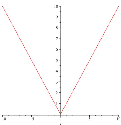
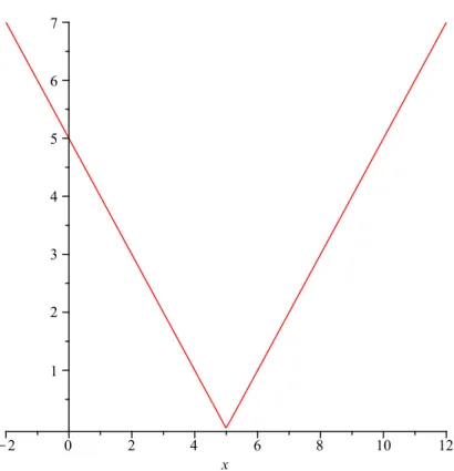
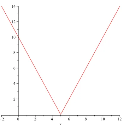
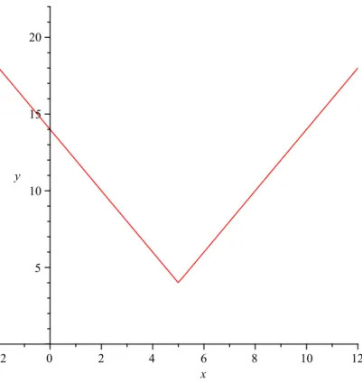
We consider an example. Let f(x) = 2|x −5|+ 4 and give the graph of this function. First take the graph of the function |x| (see Figure 1.1). Figure 1.2 shows the function |x−5|. In the third step we have the graph of 2|x−5|, see Figure 1.3. Finally, the graph of f(x) is on Figure 1.4.
We remark that this geometrical approach is useful to solve certain equations containing absolute value(s).
1.9 Exponentiation
1.9.1 Integer exponents
Let a be a real number and n a natural number. To shorten the notation for the repeated multiplication a·a·. . .·a (a appearing n times) we introduce the
Figure 1.1: Graph of the function |x|
1.9. EXPONENTIATION 23
Figure 1.2: Graph of the function |x−5|
Figure 1.3: Graph of the function 2|x−5|
1.9. EXPONENTIATION 25
Figure 1.4: Graph of the function 2|x−5|+ 4
exponential notationan, i.e.
an:=a·a·. . .·a
| {z }
ntimes
.
Here we call a the base and n the exponentor thepower. Further, put a0 := 1 and for a6= 0 puta−n := a1n for any natural number n. This way we have defined the exponentiation for any non-zero real base and any integer exponent.
Theorem 1.18. (Properties of exponentiation with integral exponents) Let m, n be integers and a, b real numbers. Further, if a or b is zero then suppose that m and n are positive. Then we have
• am·an =am+n
• aamn =am−n
• (am)n=amn
• (ab)n =anbn
• abn
= abnn
Example. Simplify the following expression containing exponentiations:
(a3)2·a4·(a2)5
a7·(a2)4 ; a6= 0.
Solution:
(a3)2·a4·(a2)5
a7·(a2)4 = a6·a4·a10 a7·a8 =
= a6+4+10
a7+8 = a20
a15 =a20−15 =a5.
Example. Simplify the following expression containing exponentiations:
(a4b−2)−2· a6b
a−2b5; a6= 0, b 6= 0.
1.9. EXPONENTIATION 27 Solution:
(a4b−2)−2· a6b
a−2b5 = (a4)−2·(b−2)−2·a6−(−2)b1−5 =a−8·b4·a8b−4 =a−8+8·b4+(−4) =a0b0 = 1.
Exercise 1.3. Simplify the following expression containing exponentiations:
a) 26·27 b) 26
24 c) 106·
1 5
6
d) (24)3 e) 84
44 f) a7·a−4
a3
g) 36·33 : 37 h) 325 i) (32)5
j) (25·34 ·53)·(24·33·52·73)
26·35·55·7 k) 242 : (24)3 l) (−3a2b4c3)2 m) 4a2b3c7·(−3ab2c5) n) −27a8b9c7
−3a4b8c7 o) 2−3a4b−5c−2 3−2a−2b−3c−1 p) 2
3(a3)2b−3c4
−1
2a4b7c−3
q) 5a0b−3(c−2)0
2−1a−3b−5d3 r) a3b−5c3 a−2b−7c s) (−2x2y−3z−1)−3·(−1x−1y4z5)2 t) 3x2(y3)2z4·2(x3y2z)3 u) a42(b3)2 a23b22
1.9.2 Radicals
Definition 1.19. Let a, b be real numbers, n a natural number. Suppose that if n is even, then a and b are positive. Then the nth root of a is denoted by √n
a and is defined by
√n
a=b if and only if a=bn. For √2
a we use the notation √ a.
Example.
√4 = 2, √3
125 = 5, √5
−32 =−2, √4
−16 has no sense (it is not a real number) Theorem 1.20. (Properties of radicals) If n, k are positive integers and a, b are positive real numbers, then we have
1). √n
an = (√n
a)n =a 2). √k
an= (√k a)n 3). √n
a√k
a= nk√ an+k 4). √n√kaa = nk√
an−k 5). pk √n
a = pn √k
a= nk√ a 6). √n
a√n b = √n
ab 7). n√n√a
b = pn a
b
Remark. The above statements are not necessarily true for the case when a, b might be negative. In one hand, for evenn some of the expressions above have no sense in the set of real numbers. On the other hand, some of the above statements may be modified for the case of negative values ofa, b.
In the case of statement 1) of Theorem 1.20 for evenn and negativeawe would have √n
an =|a|=−a, while (√n
a)n has no sense over the real numbers.
Example. Write the following expression using only one root sign:
r a3
q a2√4
a3; a≥0.
Solution:
r a3
q a2√4
a3 = r
3
q
a3·a2√4 a3 = 6
q a5√4
a3 = 6 q
p4
(a5)4·a3 = 24√
a20·a3 = 24√ a23. Example. Write the following expression using only one root sign:
√a·√3 a2·√4
a5; a≥0.
Solution:
√a·√3 a2·√4
a5 = 12√
a6· 12p
(a2)4· 12p
(a5)3 = 12√ a6· 12√
a8· 12√ a15
= 12√
a6·a8·a15= 12√
a6+8+15 = 12√ a29.
1.9. EXPONENTIATION 29 Exercise 1.4. Simplify the following expression containing exponentiations, where all the indeterminates are supposed to be positive:
a) 3 q√
2 b)
q
√5
3 c)
q
√3
a2 d) 3
q
√4
a2b e)
r a
q a√
a f)
r a
q a2√4
a3 g)
s x y
ry x
rx
y h) √3
a·√ b·√4
ab i)
ra b · 3
rb a ·√6
a
j) √3 xy· 5
rx y · 10
ry
x k)
s x y
3
ry x
√4
xy l) 5
s x4
r1 x
√3
x m)
q a√3
a√4
a n) √
a3·√3 a2·√6
a11 o) 5
q a√4
a p) 3
r a2
q a3√
a q) √7
a·√5 a·√3
a r) 4
r a5 3
q a2√
a
1.9.3 Rational exponents
To extend the exponentiation for rational exponents for integers m, n (n >1) we put
am/n = (a1/n)m = √n am
= √n
am. (1.2)
However, this has no sense among the real numbers when a < 0 and n is even.
Further, the laws of exponentiation with integer coefficient do not always generalize for the case of non-positive bases. For example, ((−1)2)1/2 = 1, but this is not equal to (−1)2·1/2 = −1. Thus in the sequel, whenever we use a non-integral rational exponent we have to restrict ourselves to positive bases.
Theorem 1.21. (Properties of exponentiation with rational exponents) Let r, s be rational numbers, and let a, b be positive real numbers. Then we have
1). ar·as =ar+s 2). aars =ar−s 3). a−r = a1r
4). (ar)s=ars 5). (ab)r =arbr 6). abr
= abrr
Example. Simplify the following expression:
a34b1310
·(√
a3)−3·√3
b2; a >0, b >0.
Solution:
a34b1310
·(√
a3)−3·√3 b2 =
a3410
· b1310
·p
(a3)−3·√3 b2
=a34·10·b13·10·√
a−9·√3
b2 =a152 ·b103 ·a−29 ·b23
=a152+−29 ·b103+23 =a62 ·b123 =a3b4. Exercise 1.5.
a)
a23 ·b126
a3·b2 b)
a23 ·b12−2
·a13 ·b2 c)
a32 ·b54−2
·a5 ·b3
d)
a43 ·b−199
a10·b2 e)
a25 ·b1210
a3·b4 f)
a13 ·b253
a3 ·b2 g)
a43 ·b325
a3·b2 h)
a32 ·b12−2
·a53 ·b2 i)
a27 ·b35−3
·a143 ·b73
j)
a−23 ·b146
a−4·b32 k)
a−25 ·b346
a−3·b34 l)
a−27 ·b3714
a−4·b6
Chapter 2
Algebraic expressions
2.1 Introduction to algebraic expressions
In algebra it is common to use letters to represent numbers. If a letter may represent several numbers, then it is called avariable, if it represents a fixed value (like Π = 3.141592. . .) then it is called a constant.
In mathematics variables are used in two ways. In one hand, there are variables which represent a particular number (or some particular numbers) which have not yet been identified, but which have to be found. (An example for this use is the case of equations.) Such variables are also called unknowns. A second use of the variables is to describe general relationship between numbers, operations and other mathematical objects. (An example for this is the use of variables in describing axioms of real numbers.)
Definition 2.1. (Algebraic expression)Analgebraic expressionis the result of performing a finite number of the basic operations addition, subtraction, mul- tiplication, division (except by zero), extraction of roots on a finite set of variables
31
and numbers, and use of a finite number of grouping symbols. By equivalent expressions we mean expressions which represent the same real number for all valid replacements of the variables.
Remark. In many cases our goal is to simplify a given algebraic expression such that the result is an equivalent expression to the original one, which is much simpler in form. In the process of this simplification one may use only a restricted number of transformations, namely those which preserve the equivalence of the expressions. These are mainly the transformations described in our theorems.
Example.
a2/3−ab2 a−1/3·√5
b, x2−3, x3−1 x2+x+ 1.
Definition 2.2. Here we define some basic notions connected to algebraic expr- essions:
• Atermis the product of a real number and powers of one or more variables.
The above-mentioned real number is called the coefficient.
• Two terms with the same variables rised to the same powers are called ”like terms” or ”terms of the same type”. Like terms which are added or subtracted may be ”collected” (using the distributive law) to get again a
”like term” to the original ones whose coefficient can be computed by adding or subtracting the coefficients of the original ”like terms”.
• A monomial is a term in which all variables are raised to non-negative integer powers.
• The degree of a monomial is the sum of the exponents of all unknowns in the monomial.
2.1. INTRODUCTION TO ALGEBRAIC EXPRESSIONS 33
• A polynomial is an algebraic expression which is the sum of finitely many monomials. If the polynomial consists of only one term, then it is a mono- mial, if it consist of 2,3,4 terms, then we call it a binomial, trinomial, quadrinomial, respectively.
• Thedegree of a polynomialis the maximum of the degree of all monomials of the polynomial.
• A non-constant polynomial is called univariate if it contains a single vari- able, and multivariate otherwise.
• The quotient of two algebraic expressions (with non-zero denominator) is called a fractional expression. The quotient of two polynomials is called a rational expression.
• Themain termof a univariate polynomial is its term with largest exponent.
The coefficient of the leading term of a univariate polynomial is called the leading coefficient of the polynomial.
2.2 Polynomials
2.2.1 Basic operations on polynomials
Adding polynomials: To add two polynomials we build the result by including all the monomials of both polynomials and we simplify the re- sult by collecting like terms.
Subtracting polynomials: Subtraction of polynomials is performed in the same way as addition, except that first we change the sign of all the monomials of the subtrahend polynomial.
Multiplying polynomials: To multiply two polynomials we multiply all terms of the firs multiplicand polynomial by all terms of the second mul- tiplicand polynomial (one by one) and we simplify the result by collecting like terms.
Example. Let P(x, y) :=x2−3xy+ 2y3 and Q(x, y) := 2x2−3xy2+ 3y3. Then we have
(P +Q)(x, y) =(x2−3xy+ 2y3) + (2x2−3xy2+ 3y3) =
=x2−3xy+ 2y3 + 2x2−3xy2+ 3y3 = 3x2−3xy+ 5y3−3xy2, (P −Q)(x, y) =(x2−3xy+ 2y3)−(2x2−3xy2+ 3y3) =
=x2−3xy+ 2y3 −2x2+ 3xy2−3y3 =−x2−3xy−y3+ 3xy2, (P ·Q)(x, y) =(x2−3xy+ 2y3)·(2x2−3xy2+ 3y3) =
= 2x4−6x3y+ 4x2y3
| {z }
(x2−3xy+2y3)·2x2
−3x3y2+ 9x2y3−6xy5
| {z }
(x2−3xy+2y3)·(−3xy2)
+ 3x2y3−9xy4+ 6y6
| {z }
(x2−3xy+2y3)·3y3
=
= 2x4−3x3y2−6x3y+ 16x2y3−6xy5−9xy4+ 6y6
2.2. POLYNOMIALS 35 Exercise 2.1. LetP(x, y), Q(x, y) and H(x, y) be polynomials defined by
P(x, y) := x2−3xy+y2,
Q(x, y) := 2x3−x2y+ 3xy2 + 5y3, H(x, y) :=x2+ 5xy+ 3x−2xy3+y.
Compute the following expressions:
a)P(x, y) +H(x, y) b) xP(x, y) +Q(x, y) c)P(x, y)·Q(x, y) d) P(x, y)−2H(x, y)
e)P(x, y)·H(x, y) f) (P(x, y)−H(x, y))P(x, y)
Exercise 2.2. LetP(x), Q(x) and H(x) be univariate polynomials defined by
P(x) :=x2−3x+ 2,
Q(x, y) :=x3 −2x2+ 3x+ 5, H(x, y) :=x2 + 2.
Compute the following expressions:
a) P(x) +Q(x) b) xP(x) +Q(x)
c) P(x)·Q(x) d) P(x) + 2H(x)
e) P(x)·H(x) f) (P(x) +Q(x))·H(x)
g) (x·P(x) + 3·Q(x))·H(x) h) P(x) +Q(x) +H(x) i) P(x)·(Q(x) +H(x)) j) P(x)·Q(x)·H(x)
2.2.2 Division of polynomials by monomials
Division of a monomial by another monomial is done in the following steps 1). Divide the sign of the two monomials.
2). Divide the coefficients of the two monomials.
3). Divide the like variables by subtracting their exponents.
Example.
12x4y7z
−3x3y =−12
3 ·x4−3y7−1z1−0 =−4xy6z.
Exercise 2.3. Divide the following two monomials (with rational coefficients):
a) 12x3y4z by 3x2yz b) 8x2y5z3 by 4x2yz2 c) 2x7y2z4 by 4x5z3 d) 3a3b4c2 by 5a2c2
e) 6a7b5c6 by 3a5bc4 f) 20a5b2c9d9 by 25a3b2c4d7 Division of a polynomial by a monomial is done in the following steps 1). Divide each term (monomial) of the dividend polynomial
by the divisor monomial.
2). Add the results to get the resulting polynomial.
Example.
x2y3−3x5y2
x2y = x2y3
x2y + −3x5y2
x2y =y2−3x3y.
Remark. Although the formal division of two monomials can be executed always, the result of this division is a monomial only when the dividend monomial is divisible by the divisor monomial. Otherwise the result is an algebraic expression, but not a monomial. The same is true for division of polynomials by monomials, and even for division of polynomials by polynomials.
2.2. POLYNOMIALS 37
2.2.3 Euclidean division of polynomials in one variable
In this section we present the division algorithm for univariate polynomials with complex, real or rational coefficients. This procedure is a straightforward genera- lization of the long division of integers.
The steps of the Euclidean division of polynomial:
1). Write the dividend and the divisor polynomials in the following scheme
dividend polynomial divisor polynomial quotient polynomial
2). Divide the main term of the dividend by the main term of the divisor polynomial, and write the resulting monomial to the place of the quotient
3). Multiply the above resulting monomial by the divisor, change the sign of every monomial of the result, and write the resulting polynomial below the dividend.
4). Draw a horizontal line, add the dividend to the above resulting polynomial and write the result of the addition below the line.
5). Let the polynomial below the last horizontal line take the role of the dividend and repeat steps 2)-4) until the polynomial below the last horizontal line is zero or has degree strictly smaller than the degree of the divisor.
Example. Divide the polynomialf(x) = x4−3x3+5x2+x−5 byg(x) = x2−2x+2.
x4 −3x3 +5x2 +x −5 x2−2x+ 2
−x4 +2x3 −2x2 x2−x+ 1
−x3 +3x2 +x −5 x3 −2x2 +2x
x2 +3x −5
−x2 +2x −2 5x −7
Remark. If in the dividend polynomial there are missing terms of lower degrees, than it is wise to include them with coefficient 0 in the scheme, so that for their like terms there is place below them.
Example. Divide the polynomialf(x) =x4+ 5x2+x−5 byg(x) =x2−2x+ 2.
x4 +0x3 +5x2 +x −5 x2−2x+ 2
−x4 +2x3 −2x2 x2+ 2x+ 7 2x3 +3x2 +x −5
−2x3 +4x2 −4x 7x2 −3x −5
−7x2 +14x −14 11x −19
Exercise 2.4. Divide the polynomialf(x) by the polynomialg(x) using the pro-
2.2. POLYNOMIALS 39 cedure of Euclidean division:
a) f(x) :=x3+ 2x2−4x+ 2, g(x) := x2−x+ 1
b) f(x) :=x5−3x4+ 4x3+ 2x2−4x+ 2, g(x) := x2−x+ 1 c) f(x) :=x5−3x4+ 2x2 −4x+ 2, g(x) :=x2−3x+ 2 d) f(x) :=x6−3x4+ 2x2−4x+ 2, g :=x3−2x+ 1
e) f(x) :=x5−3x4+ 4x3−5x2+x+ 2 g(x) :=x2−3x+ 2 f) f(x) :=x6−64, g(x) :=x2−2x+ 4
g) f(x) :=x5−2x4−3x+ 2, g(x) :=x2−3x+ 4 h) f(x) :=x5+ 2x4−5x3+ 2, g :=x2−5x+ 2
i f(x) := x5−2x4−5x3+ 2x2−3x+ 2, g(x) :=x2−4x+ 3
j) f(x) :=x5−2x4−5x3 + 2x2−3x+ 2, g(x) := x4−3x3 +x2−4x+ 3 k) f(x) := x6+ 3x5−2x4−5x3+ 2x2−3x+ 10, g(x) :=x−1
l) f(x) :=x6+ 3x5−2x4−5x3+ 2x2−3x+ 10, g(x) :=x+ 1 m) f(x) :=x6+ 3x5−2x4−5x3+ 2x2−3x+ 10, g(x) :=x−2 n) f(x) :=x6+ 3x5−2x4−5x3+ 2x2−3x+ 10, g(x) :=x+ 2 o) f(x) :=x6+ 3x5−2x4−5x3+ 2x2−3x+ 10, g(x) :=x+ 3 p) f(x) :=x6+ 3x5−2x4−5x3+ 2x2−3x+ 10, g(x) :=x2−1 q) f(x) := x6−4x4−x3+ 3x−2, g(x) :=x−1
r) f(x) :=x6−4x4−x3+ 3x−2, g(x) :=x+ 1 s) f(x) :=x6 −4x4−x3+ 3x−2, g(x) :=x−2 t) f(x) :=x6−4x4−x3+ 3x−2, g(x) :=x+ 2 u) f(x) :=x6−4x4−x3+ 3x−2, g(x) := x−3 v) f(x) := x6−4x4−x3+ 3x−2, g(x) :=x+ 3 w) f(x) :=x6−4x4−x3+ 3x−2, g(x) := x2−x−1 x) f(x) := x6−4x4−x3+ 3x−2, g(x) :=x2−1 y) f(x) := x6−4x4−x3+ 3x−2, g(x) :=x2+x−1 z) f(x) :=x6−4x4−x3+ 3x−2, g(x) :=x2+ 2x−1
2.2.4 Horner’s scheme
In this section we consider that case of the polynomial division, when the divisor takes the formx−c. Let us consider a concrete example:
2.2. POLYNOMIALS 41 1x4 +2x3 +5x2 +x −5 x−2
−x4 +2x3 1x3 + 4x2+ 13x+ 27
4x3 +5x2 +x −5
−4x3 +8x2
13x2 +x −5
−13x2 +26x 27x −5
−27x +54 49
It is clear that in fact we only need to compute the numbers typeset by red, since they are exactly the coefficients of the quotient, and of course the remainder typeset in blue. The Horner’s scheme below gives a much simpler procedure to compute these numbers:
Theorem 2.3. (Horner’s scheme) Let f(x) = anxn+an−1xn−1+· · ·+a1x+a0
with an, . . . , a0 ∈ R, and g(x) = x−c with c ∈ R be two polynomials. Build the following table:
an an−1 . . . . ai+1 . . . . a1 a0
c bn−1 bn−2 . . . bi . . . b0 r
where
bn−1 :=an
bi :=b·bi+1+ai+1 for i=n−2, n−3, . . . ,0 r:=c·b0+a0.
(2.1)
Then the quotient of the polynomial division of f by g is the polynomial
q(x) =bn−1xn−1+bn−2xn−2+· · ·+b1x+b0,
and the remainder is the constant polynomial r. Further, we also have
f(c) = r. (2.2)
Remark. In other words the above theorem states that in Horner’s scheme the numbers in the first line are the coefficients of the polynomialf, and the numbers computed in the second line of the scheme are the following:
• the first number is the zero of the polynomial g(x) =x−c,
• the next numbers (except for the last one) are the coefficients of the quotient polynomial of the polynomial division off byg,
• the last number is the remainder of the above division, but it is also the value of the polynomialf(x) at x=c.
Example. Now we divide the polynomial f(x) = x4 + 2x3+ 5x2+x−5 by the polynomialx−2 using Horner’s scheme. The first place in the first line is empty, then we list the coefficients of f. Then we solve the equation
x−2 = 0
to get x= 2, thus the first element in the second line of the Horner’s scheme will be 2. Then we compute the consecutive elements of the second line using (2.1) to get
1 2 5 1 −5
2 1 4 13 27 49
This means that f(x) = (x−2)(x3+ 4x2+ 13x+ 27) + 49.
2.2. POLYNOMIALS 43 Remark. If in the dividend polynomial there are missing terms of lower degrees, than it is compulsory to include the coefficients of these terms (i.e. 0-s) in the upper row of the Horner’s scheme.
Example. Divide the polynomial f(x) = x4−5x2+x−5 by the polynomialx+ 2 using Horner’s scheme. The first place in the first row is empty, then we list the coefficients of f, including the coefficient 0 ofx3. Then we solve the equation
x+ 2 = 0
to getx=−2, thus the first element in the second row of the Horner’s scheme will be 2. Then we compute the consecutive elements of the second line using (2.1) to get
1 0 −5 1 −5
−2 1 −2 −1 3 −11
This means that f(x) = (x+ 2)(x3−2x2 −x+ 3) + (−11).
Exercise 2.5. Divide the polynomial f(x) by the monic linear polynomial g(x)
using Horner’s scheme:
a)f(x) = x5−2x4+x3−3x2+ 2x−5, g(x) = x+ 1 b)f(x) = x5−5x4+ 3x3−2x2+ 2x−3, g(x) =x−2 c)f(x) = x5−5x4+ 3x3−2x2+ 2x−3, g(x) =x+ 2 d)f(x) = x7−5x6+ 2x5−4x4−x3+ 3x−2, g(x) =x−1 e)f(x) = x7−5x6+ 2x5−4x4−x3+ 3x−2, g(x) =x+ 1 f) f(x) = x7−5x6 + 2x5−4x4−x3+ 3x−2, g(x) =x−2 g)f(x) = x7−5x6+ 2x5−4x4−x3+ 3x−2, g(x) =x+ 2 h)f(x) = x6−2, g(x) =x−1
i)f(x) =x6−2, g(x) =x−2 j) f(x) =x6 −2, g(x) = x+ 2
k) f(x) :=x6+ 3x5−2x4 −5x3+ 2x2−3x+ 10, g(x) :=x−1 l)f(x) :=x6+ 3x5−2x4−5x3+ 2x2−3x+ 10, g(x) :=x+ 1 m) f(x) := x6+ 3x5−2x4−5x3+ 2x2−3x+ 10, g(x) :=x−2 n)f(x) := x6+ 3x5−2x4−5x3+ 2x2−3x+ 10, g(x) :=x+ 2 o)f(x) := x6+ 3x5−2x4−5x3+ 2x2−3x+ 10, g(x) :=x+ 3 p)f(x) := x7−x5+x3 −x, g(x) := x+ 1
q) f(x) :=x6−4x4−x3+ 3x−2, g(x) :=x−1 r)f(x) :=x6−4x4−x3+ 3x−2, g(x) :=x+ 1 s)f(x) :=x6−4x4−x3+ 3x−2, g(x) :=x−2 t)f(x) :=x6−4x4−x3+ 3x−2, g(x) :=x+ 2 u)f(x) := x6−4x4 −x3 + 3x−2, g(x) :=x−3 v) f(x) :=x6−4x4−x3+ 3x−2, g(x) :=x+ 3,
w)f(x) = x7+ 3x6+ 2x5−3x4+x3−5x2−3x+ 4, g(x) =x+ 1 x) f(x) =x7+ 3x6+ 2x5−3x4+x3−5x2−3x+ 4, g(x) =x−1 y) f(x) =x7+ 3x6+ 2x5−3x4+x3−5x2−3x+ 4, g(x) =x+ 2 z)f(x) = x7+ 3x6+ 2x5−3x4+x3−5x2−3x+ 6, g(x) = x+ 1
2.2. POLYNOMIALS 45 Exercise 2.6. Decide using Horner’s scheme if the below polynomial f(x) is di- visible by the polynomial g(x) or not, and if the answer is yes, then compute the quotient f(x)g(x), and if the answer is no, then compute the quotient and the remainder