Economics, Szeged, https://doi.org/10.14232/eucrge.2020.proc.9
Livestock product supply and factor demand responsiveness:
A farm-level analysis in the Southern Rangelands of Kenya
John Kibara Manyeki – Izabella Szakálné Kanó – Balázs Kotosz
Despite there being incredible challenges in enhancing livestock development in Kenya, this article isolates product supply and factors input demand responsiveness as the main constraints facing the smallholder. A flexible-Translog profit function permits the application of dual theory in the analysis of livestock product supply and factor demand responsiveness using farm-level household data. The results indicate that own-price elasticities were elastic for cattle, while goat and sheep were inelastic. Cross-price and scale elasticities were found to be within inelastic range in all cases, with the goat being a preferred substitute for cattle.
All factor inputs demand elasticities were inelastic with the exception of elastic cattle output prices and labour cost. Thus, the recommended policy option would be supportive pro-pastoral price policies, enhanced investment in pastureland improvement and an increasing wage rate, since these assume key significance in improving the livestock production/marketing.
Keywords: duality, own-price elasticity, cross-price elasticity, livestock, Kenya.
1. Introduction
In the ongoing debate over implicit taxation through changes in macroeconomic policies and movement quarantines in the Kenyan livestock trade (Ronge et al. 2005), economic analysis of potential output, price, and trade responses have played an essential role in the negotiation process. The markets in which livestock compete are increasingly influenced by intense livestock inflow from neighbouring countries of up to 25% (Behnke–Muthami 2011), rapid technological change (Thornton 2010, Collier–Dercon 2014), shorter product production life-cycles, and customers increasingly unwilling to settle for sometimes mass-livestock produced items of limited value. The “new breed of customer” (Robinson–Pozzi 2011), who demands greater responsiveness (Kariuki et al. 2013), and a new competitive environment (Yego–Siahi, 2018), which exposes local livestock farmers to competition, forms a new scenario that needs to be addressed. In this new scenario, responsiveness may be one of the essential options required for farmers to achieve competitive advantage. A critical element in this analysis is knowledge of the responsiveness of Kenyan livestock output to the own- and cross-price elasticities of supply, and input factor demand (FD).
While the available studies have given some insight into output-price responsiveness (e.g., Nyariki 2009, Manyeki et al. 2016, Mathini et al. 2017), they have not fully extended our understanding of factor substitution/complementarity in the livestock sector. One of the shortcomings inherent in their approach as cited by Debertin (2012) was that input demand and output supply (OS) are parts of a
comprehensive system, hence estimating the latter alone may provide inefficient results for the underlying supply relationship. Therefore, it is desirable to determine the interlinked livestock OS and factor input demand equations simultaneously. The utility of these few studies directly addressing livestock production and marketing behaviour is limited because, in most cases, they restrict themselves to only a few livestock products, targeting specific small regions, most employ estimation samples that are small, and some fail to meet behavioural (curvature) conditions necessary for the approaches used, partially because they aggregate many agricultural variables that have been criticised for obscuring the behaviour of individual input variables (Nyariki 2009, Olwande et al. 2009, Zhou–Staatz 2016, Manyeki et al. 2016, Tothmihaly 2018). This study was designed to fill a portion of this information gap, and a profit function analysis based on duality theory was the procedure employed to simultaneously derive these systems of OS and FD equations, and use it on extensive household-farm level data collected in the entire difficult terrain of the southern rangelands of Kenya.
Such robust estimation of farmer responsiveness was deemed to be important in informing the policy-setting process because it focuses on many decisions facing farmers, such as what portion of resources to devote to livestock production (land, capital, labour both family and hired) and policy incentives to stimulate livestock product market participation. The discussion proceeds in the next sections with a theoretical framework that set the empirical model used in analyses. The data and estimation procedure are then presented, followed by the analysis and discussion of results.
2. Theoretical framework
This paper applies duality theory (Shepard 1954) and uses it to analyse livestock product supply and input responses sequentially. The concept behind dual method (Shepard 1954, Debertin 2012) implies that the shape of the total variable cost function is closely linked to the shape of the production function that underlies it. If input prices are constant, all the information about the shape of the variable cost function is contained in the equation for the underlying production function.
Therefore, in the dual theoretical framework, two short-run versions of duality can be generated; if it is assumed that either output level or input levels are known and constant. In the former case (i.e. constant output), objective function simplifies to the minimisation of cost subject to the requirement of generating the given output level.
In the latter case of known and fixed input levels, the objective function simplifies to maximisation of revenue subject to the use of the given input levels. In either case, corresponding marginality conditions may be derived for these short-run variants of the profit maximisation or cost minimisation problem.
While the goal of the study is to use dual approach to obtain a system of OS and FD equations, the possible estimation problems are associated with production function (Chambers 1988, Sadoulet and de Janvry 1995). The reason for adopting a profit maximisation approach (maximum profit attainable given the inputs, outputs, and prices of the inputs) over the cost minimisation approach, is that the latter assumes that output levels are not affected by factor price changes and, thus, the indirect effect of factor price changes (via output levels) on FDs are ignored (e.g., Olwande et al.
2009, Debertin 2012). Indeed, the inclusion of output levels as explanatory variables in cost minimisation function may lead to simultaneous equation biases if output levels are not indeed exogenous. The profit function approach overcomes most of these problems, although it requires a stronger behavioural assumption. The FDs estimated using a profit function framework allow one to measure input substitution and output scale effects of factor price changes. Additionally, one can measure the cross effects of output price changes on FDs, and vice versa, as well as OS responses and their cross-price effects. Finally, the profit function framework allows the estimation of multi-output technologies in a much simpler way than a cost function or a transformation function.
The econometric application of the variable profit/cost function represents a significant step forward towards generating an appropriate system of agricultural OS and input demand functions which are crucial for the application of economic theory to farm development policy (Lau–Yotopoulos 1972, Yotopoulos et al. 1976, Sidhu–
Baanante 1981). To examine the behavioural decisions of smallholder pastoral livestock producers on output and input use, specifically on their responsiveness, farmers were assumed to maximise restricted profit conditional on a convex production possibility set or technology T expressed by
𝜋(𝑃, 𝑊; 𝑍) = 𝑀𝑎𝑥
𝑄,𝑋 {𝑝𝑄 − 𝑤𝑋|𝐹(𝑄, 𝑋; 𝑍) ∈ 𝑇} (1) Subject to the constraint that 𝜋 = 𝑅 − 𝐶 ≥ 𝜋∗
Where, 𝑅 = 𝑝𝑄 is the gross receipts, and 𝐶 = 𝑤(. ) is the cost functional structure. Q and X are vectors of quantities of outputs, and variable inputs, and 𝑃 and 𝑊 are the corresponding vectors of output and input prices respectively; Z denotes the amount of fixed factors inputs(e.g., land, capital). The profit function, 𝜋(. ), is assumed to be non-decreasing in p, non-increasing in w, linear homogeneous and convex in p and w.
The function 𝜋 = 𝑅 − 𝐶 ≥ 𝜋∗ shows the farmer specific minimum acceptable profit level, 𝜋∗, referred to as lower bound, and capture satisfictory behaviour due to information asymmetry in the market.
In this profit function, the major impediments are the variable inputs cost structure, 𝑤(. ) given the independence of the production possibility sets and, therefore, the concept of normalised restricted profit function was adopted.
Normalisation has the purpose of removing any money illusion (in other words, producers respond to relative price changes) and also reduces the demand on degrees of freedom, by effectively reducing the number of equations and parameters to estimate. In the case of a single output, a normalised restricted profit function (defined as the ratio of the restricted profit function to the price of the output), π*, can be specified. In the case of multi-output normalised profit function, the numéraire is the output price of the nth commodity and, following Färe and Primont (1995), the restricted profit function was specified as:
𝜋𝑖∗= 𝜋𝑖∗(𝑃∗, 𝑊∗; 𝑍) (2)
Where normalised profit, output prices and input prices are defined by 𝜋𝑖∗= 𝜋 𝑝⁄ , 𝑃𝑖∗= 𝑃𝑖⁄𝑃 and 𝑊𝑖∗= 𝑊𝑖⁄𝑃 respectively. Here, P is the minimum acceptable price for cattle and sheep and goat outputs (shoat hereafter) satisfactory to a smallholder household i – referred to as farm gate price. Differentiating the normalised profit function with respect to prices of outputs and inputs respectively would yield the supply function of output and demand functions for input.
3. The empirical model
To implement this process empirically, it is necessary first to specify a profit function form. In the literature, the use of several flexible, functional forms to give a second- order Taylor approximation to an arbitrary (true) functional form such as Translog by Christensen et al. (1973), generalised Leontief by Diewert (1973), generalised symmetric McFadden by Diewert and Wales (1987), and normalised quadratic by Lau (1976) permits the application of the duality theory for a more disaggregated analysis such as livestock sector of Kenya. To formulate an effective livestock production and marketing policies, one needs reliable empirical knowledge about the degree of responsiveness of demand and supply for factors and products, to relative prices and technological changes. The normalised Translog version of the profit function was considered to be one of the general functions for the approximation of production function and simultaneously for estimation of OS and FD responsiveness since they are closely interlinked to each other. The logarithmic Taylor series expansion of normalised profit function (equation 2) can be written as:
𝐿𝑛𝜋𝑖∗(𝑃𝑖∗, 𝑊𝑗∗; 𝑍𝑘) = 𝛼0+ ∑𝑁𝑖=1𝛽𝑖𝐿𝑛𝑃𝑖∗+ ∑𝑀𝑗=1𝛾𝑗𝐿𝑛𝑊𝑗∗+ ∑𝐾𝑘=1𝛿𝑘𝐿𝑛𝑍𝑘+
∑𝑁𝑖=1∑𝑀𝑗=1𝜗𝑖𝑗𝐿𝑛𝑃𝑖∗𝐿𝑛𝑊𝑗∗+ ∑𝑁𝑖=1∑𝐾𝑘=1𝜃𝑖𝑘𝐿𝑛𝑃𝑖∗𝐿𝑛𝑍𝑘+
∑𝑀𝑗=1∑𝐾𝑘=1𝜉𝑗𝑘𝐿𝑛𝑊𝑗∗𝐿𝑛𝑍𝑘+12(∑𝑁𝑖=1∑𝑁ℎ=1𝜏𝑖ℎ𝐿𝑛𝑃𝑖∗𝐿𝑛𝑃ℎ∗+
∑𝑀𝑗=1∑𝑀𝑙=1𝜙𝑖𝑙𝐿𝑛𝑊𝑗∗𝐿𝑛𝑊𝑙∗+ ∑𝐾𝑘=1∑𝐾𝑢=1𝜓𝑖𝑢𝐿𝑛𝑍𝑘𝐿𝑛𝑍𝑢) (3) Where, subscripts i, stand for output and run from 1 to 𝑁; 1, subscripts j and l stand for variable inputs (prices) and run from 1 to 𝑀; 2, subscripts k and u stand for fixed inputs and run from 1 to 𝐾;3, 𝑃𝑖 and 𝑊𝑗 are output and input prizes respectively; 𝑍𝑘 denotes the quantity of factor 𝑘 that are assumed to be fixed in the short term (e.g., area of pasture land, the value of capital assets = household income).The term, 𝜋𝑖∗, is the restricted profit of ith product normalised by the average product price 𝑃𝑖; 𝑃𝑗∗ is the normalised price of multi-output technologies, normalised by the output price 𝑃𝑖, that is, 𝑃𝑗∗ = 𝑃𝑗⁄𝑃𝑖 where i, j= cattle price, sheep, and goat price; 𝑷∗; 𝑾∗; 𝒁 are
1 In our case 𝑁 = 3, because we have three outputs: cattle, goat, and sheep.
2 In our case 𝑀 = 1, because we have only one variable input: Labour.
3 In our case 𝐾 = 2, because we have two fixed inputs: Pasture land area and Household income.
vectors of these variables; Coefficients 𝛼𝑖0 , 𝛽𝑖𝑗 , 𝛾𝑖𝑘 , 𝛿𝑖ℎ, 𝜗𝑖𝑗𝑘 , 𝜃𝑖𝑗ℎ, 𝜉𝑖𝑘ℎ , 𝜏𝑖𝑗𝑙, 𝜙𝑖𝑘𝑚, and 𝜓𝑖ℎ𝑛 are the parameters to be estimated and Ln = natural logarithm.
Using Hotelling’s Lemma, the first-order derivatives of equation (3) with respect to normalised prices of variable outputs i yield a system the OS (Y) equations:
𝑌(𝑃𝑖∗, 𝑊𝑗∗; 𝑍𝑘) =𝜕𝐿𝑛𝜋𝑖∗(𝑃𝑖∗,𝑊𝑗∗;𝑍𝑘)
𝜕𝐿𝑛𝑃𝑖∗ = 𝛽𝑖+ ∑𝑀𝑗=1𝜗𝑖𝑗𝐿𝑛𝑊𝑗∗+ ∑𝐾𝑘=1𝜃𝑖𝑘𝐿𝑛𝑍𝑘+
∑𝑁ℎ=1𝐿𝑛𝑃ℎ∗+ 𝜀 (4)
Further, a system of inverse input demand equations that represent technological change is obtained by differentiating equation 3 with respect to normalised variable input prices 𝑊𝑖∗ and fixed factor 𝑍𝑘, yielding a system of inverse variable inputs equations X and shadow-value equations, Q expressed as:
𝑋(𝑃𝑖∗, 𝑊𝑗∗; 𝑍𝑘) = −𝜕𝐿𝑛𝜋𝑖∗(𝑃𝑖∗,𝑊𝑗∗;𝑍𝑘)
𝜕𝐿𝑛𝑊𝑖∗ = 𝛾𝑗+ ∑𝑁𝑖=1𝜗𝑖𝑗𝐿𝑛𝑃𝑖∗+ ∑𝐾𝑘=1𝜉𝑗𝑘𝐿𝑛𝑍𝑘+
∑𝑀𝑙=1𝜙𝑖𝑙𝐿𝑛𝑊𝑙∗+ 𝑒 (5)
𝑄(𝑃𝑖∗, 𝑊𝑗∗; 𝑍𝑘) = −𝜕𝐿𝑛𝜋𝑖
∗(𝑃𝑖∗,𝑊𝑗∗;𝑍𝑘)
𝜕𝐿𝑛𝑍𝑘 = 𝛿𝑘+ ∑𝑁𝑖=1𝜃𝑖𝑘𝐿𝑛𝑃𝑖∗+ ∑𝑀𝑗=1𝜉𝑗𝑘𝐿𝑛𝑊𝑗∗+
∑𝐾𝑢=1𝜓𝑖𝑢𝐿𝑛𝑍𝑢+ 𝜂 (6)
These systems of supply and demand response equations (4–6) show the relation between OS and input demand to the output prices, input prices and the quantities of fixed factors respectively. To exhibit the properties of a well-behaved profit function, equation 3 must be non-decreasing in output price (𝛽𝑖 ≥ 0, for i=cattle, sheep, and goat outputs), non-increasing in input prices ( 𝛿𝑘 ≤ 0, for k=pasture land, capital, and labour, and 𝛾𝑗 ≤ 0 for labour price) and symmetry constraints are imposed by ensuring equality of cross derivative (e.g., 𝜗𝑖𝑗 = 𝜗𝑗𝑖 𝜗𝑖𝑗for all i, j; i ≠ j, 𝜃𝑖𝑘 = 𝜃𝑘𝑖 for all i, k; i ≠ k and 𝜉𝑗𝑘= 𝜉𝑘𝑗 for all j, k; j ≠ k). This implies that all own price responsiveness (elasticities) are expected to be positive for OS and negative for input variable costs, and less than unity. However, the cross-price elasticities are expected to be indeterministic such that a negative sign implies a degree of substitutability with a positive sign indicate a degree of complementarity. The homogeneity and algebra are automatically maintained by constructing a normalised Translog profit function.
Similarly, the OS functions (4) and inputs demand functions (5–6) exhibit theoretical restrictions reflecting the properties of the profit functions.
The empirical model consists of equations 4–6 with symmetry imposed and truncated normal distribution (with mean μ and standard deviation σ appended iid error terms {ε, 𝑒, 𝜂}). In total, a system of nine equations was derived from the normalised profit function, and the variables were converted to logs before subjected to analysis. The nine equations considered included three OS (each for cattle, sheep, and goat) and six FD – two for each livestock product. Variable inputs include labour
(a composite of family and hired labour) and two fixed inputs presented by a total area under pasture measured in hectares and farm capital asset expressed in monetary value. With regards to fixed input demand response, size of improved pastures land demand equation was regarded as important in production decisions, improvement is an extra production cost in the short-run, but in the long-run, help reduces production cost and increases profit, and thus stimulates higher supply. The size and quality of pastureland form an extra cost to livestock production in the short run. Therefore, a negative effect is expected, but in the long-run, help reduces production cost and increases profit, thus stimulating higher supply. When it comes to variable input demand equation, we only included labour since data on other variables such as costs of livestock supplies (e.g. drugs, vaccines) and veterinary services/consultancies was not available as farmers in the study areas don’t keep records and estimating the same for the last year proved very difficult. Labour variable was captured in man-days and included both hired, and family labour, and the prevailing government wage rates were used to estimate the cost of labour. As such, the more the man-days holding the marginal product of labour constant, the more the production costs and, therefore, the less the expected profit and vice versa.
4. Data and estimation procedure
The dataset used was the Kenyan Household Survey which was a nation-wide survey of rural households that was conducted during September and October 2013. The survey was undertaken in the 47 counties across the country, of which 12,651 agricultural households were randomly selected from a total of 6,324,819 (GoK 2010) by applying a systematic Probability Proportional to Size sampling technique and considering the prominent production systems (agro-ecological zones) found in Kenya. The sampling frame comprises 1512 households interviewed in Garissa, Kajiado, Kilifi, Kitui, Kwale, Lamu, Makueni, Narok, Taita-Taveta, and Tana-River counties. These counties were deemed representative of many livestock production zones in Kenya. Outputs and inputs variable data were extrapolated based on the prevailing market values as of 2013.
To estimate the OS and FD functions, a maximum likelihood estimation (MLE) technique that involved a two-stage approach was used. In the first step, it was necessary to assume a stochastic structure and, thus any deviations of the observed profit, OS and FD from their profit-maximising levels were due to random errors in optimisation and that the disturbances were additive and followed a multivariate normal distribution with a zero mean (μ), and a constant contemporaneous covariance matrix (Σ) expressed in shorthand notation as X∼N (μ, Σ). Then, by taking the first- order derivative using Hotelling’s Lemma, we derived a system of five equations from the normalised profit function.
The second phase of analysis involved the estimation of derived systems of OS and FD equations, and a truncated regression analysis was adopted. An MLE technique was involved assuming truncated (at zero) normal distribution, which is the probability distribution of a normally distributed random variable with mean μ and
standard deviation σ (Wooldridge 2010). To simplify the mathematical expression of the functional form both output and variable input quantities are included in the vector 𝑦𝑖. Thus, 𝑦𝑖 is a ‘netput’ vector where positive values are outputs, and negative values are variable inputs. In addition, both output and input prices and both fixed inputs are included in the vector xi. For this study, to avoid bias in the estimation, sample selection was determined solely by the value of x variable, and the density of the truncated normal distribution of the i-th observation was expressed by
𝐿𝑖 =
1
𝜎𝜙(𝑦𝑖−𝑥𝑖𝜎′𝛽) Φ(𝑥𝑖′𝛽𝜎)
(7)
Where 𝜙 and Φ are the density and distribution functions of the standard normal distribution. The log-likelihood function is given by
𝐿𝑜𝑔𝐿(𝛽, 𝜎) = ∑𝑁𝑖=1𝐿𝑜𝑔𝐿𝑖 = −𝑁2[𝐿𝑜𝑔(2𝜋)] + 𝐿𝑜𝑔(𝜎2) −2𝜎12∑𝑁𝑖=1𝜀𝑖2−
∑𝑁𝑖=1𝐿𝑜𝑔 [Φ (𝑥𝜎𝑖′𝛽)], (8)
Where the values of (β,σ) that maximise LogL are the maximum likelihood estimators of the truncated regression. Using the parameter estimates, and assuming output prices and input prices are defined by 𝑥̅𝑗= 𝑃𝑖⁄𝑃 and 𝑥̅𝑗 = 𝑊𝑖⁄𝑃 respectively, the own-price responsiveness was calculated at the population means using:
𝑒𝑖𝑗 = 𝛽𝑖𝑗∗𝑥̅𝑗
𝑦̅𝑖 for 𝑖 = 𝑗, j = cattle, sheep, goat, labour, and land, (9a) And the cross-price responsiveness:
(9b) 𝑒𝑖𝑗 = 𝛽𝑖𝑗∗𝑥̅𝑗
𝑦̅𝑖 for 𝑖 ≠ 𝑗, j = cattle, sheep, goat, labour, and land, (9b) For own price response, 𝑒𝑖𝑗 represent the per cent change in quantity demand (supplied) of input (output) of type i in response to a 1% change in the prices of input (output) of type i. Likewise, for the cross-price response, 𝑒𝑖𝑗 represent the per cent change in quantity demand (supplied) of input (output) of type i in response to a 1%
change in prices of input (output) type j, holding all prices of other than of the j-th input (output) constant. Positive (negative) value of cross-price elasticities indicated that i and j were substitutes (complements). Additionally, following Färe et al. (1986), we estimated responsiveness of scale via the output-oriented measure of scale elasticity.
5. Empirical results
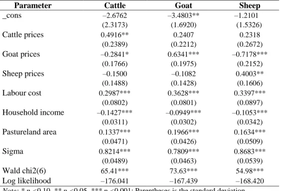
Parameter estimates from the derived system of OS and input demand are given in Tables 1 to 4. With three outputs and two inputs in the model, only 6 and 5 parameters respectively are freely estimated. Tables 2 and 4 give the elasticity computed (with their corresponding standard error) of the three outputs supply and three input demand equations for the farm-household data. In all cases, the output and inputs prices were normalised and directly included in the equations. In Table 1, the results of the coefficient estimate for OS and labour demand are found to be robust in all cases. The signs of the own-price coefficient estimate for livestock supply are all theoretically consistent and significant at 1% and 5% level (Table 1), with a positive supply elasticity (Table 2). The result indicates that own-prices are inelastic for goat and sheep. The most inelastic being sheep followed by the goat. Own-price elasticity is relatively elastic for cattle.
Cross-price elasticities were found to be in the inelastic range in all cases which indicate that a price change will result in a relatively small uptick in supply of livestock products. The cross-price elasticities indicate that cattle can be a substitute for sheep and goat, and sheep and goat a complement for cattle. Moreover, cattle output is less price responsive to goat and sheep prices than goat, and sheep output is to cattle prices. The only cross-price elasticity that was significant was between cattle and goat prices and sheep and goat prices. The cross-price elasticities for sheep and goat are similar (as they are both negatives), while those between cattle and goat and cattle and sheep output are indeterministic.
Outputs response to variable input was measured by the cost of labour normalised by output price of type i, the individual household income and the size of improved pastureland in hectares. Labour price portrayed a cross-relation to herd size and the greater the labour costs, ceteris paribus, the larger the herd size, and this would translate to more livestock available for marketing. The livestock supply equations had unexpected negative elasticity with respect to the household income. In contrast, the most essential fixed input in terms of livestock output response was the size of improved pasture land. Pastureland was specified as the total hectares of (natural or enhanced) land pasture and in this case, captured technological change that is regarded as valuable in production decisions.
The elements in the row labelled ‘scale elasticities’ in Table 2 reflects the OS response to a change in all exogenous variables combined. Generally, the scale elasticities for the three livestock products were less than one (though not less than zero, giving the possibility of free disposal), which indicates decreasing returns to scale.
However, goat output seems to be more responsive to factor inputs than cattle and sheep output are. The possible explanation to this finding is, in pastoralist areas, where frequent droughts and diseases are experienced, goats are becoming attractive since they are hardier, can easily be de-stocked during drought and re-stocked afterwards, hence reducing the losses due to starvation (Degen 2007). The estimates of sigma square (𝜎2) are significantly different from zero at 1% level of significance, implying a good fit and correctness of the specified distribution assumptions of the composite error term.
The Wald Chi-square value (Wald chi2(6)) showed that statistical tests are highly significant (P < 0.000), suggesting that the model had strong explanatory power.
Table 1 Parameter estimates of OS equations for the southern rangeland of Kenya
Parameter Cattle Goat Sheep
_cons –2.6762
(2.3173)
–3.4803**
(1.6920)
–1.2101 (1.5326)
Cattle prices 0.4916**
(0.2389)
0.2407 (0.2212)
0.2318 (0.2672)
Goat prices –0.2841*
(0.1766)
0.6341***
(0.1975)
–0.7178***
(0.2152)
Sheep prices –0.1500
(0.1488)
–0.1082 (0.1428)
0.4003**
(0.1606)
Labour cost 0.2987***
(0.0802)
0.3628***
(0.0801)
0.3397***
(0.0897) Household income –0.1427***
(0.0311)
–0.0949***
(0.0302)
–0.1053***
(0.0342) Pastureland area 0.1337***
(0.0471)
0.1966***
(0.0426)
0.1634***
(0.0509)
Sigma 0.8214***
(0.0489)
0.7809***
(0.0463)
0.8683***
(0.0539)
Wald chi2(6) 65.41*** 73.63*** 54.98***
Log likelihood –176.041 –167.439 –168.420 Note: * p <0.10, ** p <0.05, *** p <0.001; Parentheses is the standard deviation.
Source: Author’s construction.
Table 2 Livestock products OS elasticity
With respect to: Cattle Goat Sheep
Cattle Price 0.689
(0.911)
0.077 (0.299)
0.108 (0.443)
Goat Price –0.0052
(0.023)
0.565 (0.780)
–0.081 (0.435)
Sheep Price –0.0015
(0.010)
–0.006 (0.089)
0.221 (0.276)
Labour Cost 0.120
(0.454)
0.375 (1.366)
0.440 (1.394) Household Income –0.156
(0.197)
–0.058 (0.092)
–0.042 (0.064)
Pastureland 0.040
(0.040)
0.028 (0.053)
0.027 (0.041) Scale elasticities 0.686
(0.273)
0.981 (0.447)
0.673 (0.442) Note: Parentheses is the standard deviation.
Source: Author’s construction.
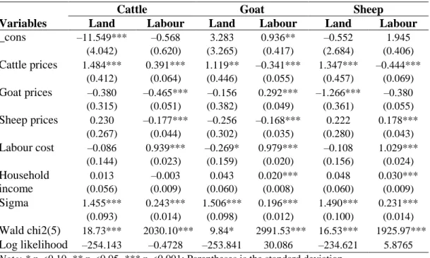
Tables 3 and 4 contain the parameter estimates and price elasticities for the FD system, respectively. All factor input demand elasticities were found to be in the inelastic range with the exception of cattle output prices and labour cost, which was elastic for land demand in cattle and goat production enterprises respectively.
Estimates for labour input demand equations were robust, though less precise in many cases than that of pastureland counterpart. With regards to output prices, all production enterprise showed an elastic response of pastureland demand to cattle output price. However, labour demand was reasonably responsive to cattle output prices in the cattle production enterprise. The situation with regards to goat and sheep output prices on FDs is opposite except for labour and land demand response to goat and sheep output prices respectively, which is relatively inelastic. The pastureland response in the goat and sheep production enterprise are similar and relatively elastic, an increase in sheep and cattle output prices puts substantial positive pressure on land demand, and indeed, this can explain the great effect shown on sheep and cattle supply. Increases in goat output price would encourage the expansion in demand for labour under goat production enterprise, while it would result in a reduction in pastureland demand in all cases.
When it comes to the effect of labour costs on labour demand responsiveness, it should be pointed out that demand for labour was very significant and influenced much more by a change in labour prices than by a change in livestock output prices.
The situation is the opposite with a relatively elastic response of pastureland demand on labour costs in the goat production enterprise, but an inelastic response to cattle and sheep production enterprises. This strong elasticity of labour costs on pastureland demand equation for goat production possibly may be associated to the fact that goats are browsers, unlike cattle and sheep, which are heavy grazers. The results have important implications for agricultural research and development policies for developing countries such as Kenya. The availability of labour is a more serious constraint owing to its relatively low elasticities but very significant across all livestock type.
Finally, household income portrayed a positive effect in factor input demand elasticities in all cases with a relatively low negative impact on labour demand recorded in the cattle production enterprise. The income effect can be observed under two scenarios: if a household aggregate level of income increases or if the relative cost of expanding pastureland or wage for labour decreases. Both situations increase the amount of discretionary income available, so does the quantity of pasture and labour. FD in sheep production enterprise was relatively more responsive to changes in household income. The estimates of sigma square (𝜎2) are significantly different from zero at 1% level of significance, implying a good fit of the specified distribution assumptions of the composite error term, and the Wald chi2(5) showed that statistical tests are significant, suggesting that the model had strong explanatory power.
Table 3 Parameter estimates of input demand equations for the livestock production Variables
Cattle Goat Sheep
Land Labour Land Labour Land Labour
_cons –11.549***
(4.042)
–0.568 (0.620)
3.283 (3.265)
0.936**
(0.417)
–0.552 (2.684)
1.945 (0.406) Cattle prices 1.484***
(0.412)
0.391***
(0.064)
1.119**
(0.446)
–0.341***
(0.055)
1.347***
(0.457)
–0.444***
(0.069) Goat prices –0.380
(0.315)
–0.465***
(0.051)
–0.156 (0.382)
0.292***
(0.049)
–1.266***
(0.361)
–0.380 (0.055) Sheep prices 0.230
(0.267)
–0.177***
(0.044)
–0.256 (0.302)
–0.168***
(0.035)
0.222 (0.280)
0.178***
(0.043) Labour cost –0.086
(0.144)
0.939***
(0.023)
–0.269*
(0.159)
0.979***
(0.020)
–0.108 (0.156)
1.029***
(0.024) Household
income
0.013 (0.056)
–0.003 (0.009)
0.043 (0.060)
0.020***
(0.008)
0.048 (0.060)
0.030***
(0.009)
Sigma 1.455***
(0.093)
0.243***
(0.014)
1.506***
(0.098)
0.196***
(0.012)
1.490***
(0.100)
0.231***
(0.014) Wald chi2(5) 18.73*** 2030.10*** 9.84* 2991.53*** 16.53*** 1925.97***
Log likelihood –254.143 –0.4728 –253.841 30.086 –234.621 5.8765 Note: * p <0.10, ** p <0.05, *** p <0.001; Parentheses is the standard deviation.
Source: Author’s construction.
Table 4 Factor input demand elasticity for livestock production With respect
to:
Cattle Goat Sheep
Land Labour Land Labour Land Labour Cattle Price 2.322
(3.436)
0.059 (0.096)
0.882 (3.959)
–0.021 (0.108)
0.833 (2.126)
–0.018 (0.034) Goat Price –0.006
(0.017)
–0.001 (0.006)
–0.594 (0.618)
0.085 (0.142)
–0.255 (0.565)
–0.006 (0.017) Sheep Price 0.002
(0.008)
–0.0002 (0.0005)
–0.189 (0.467)
–0.002 (0.028)
0.401 (0.685)
0.029 (0.071) Labour Cost –0.047
(0.114)
0.016 (0.017)
–1.185 (2.371)
0.088 (0.048)
–0.322 (0.970)
0.086 (0.079) Household
Income
0.011 (0.017)
–0.0003 (0.0005)
0.008 (0.013)
0.004 (0.006)
0.047 (0.081)
0.003 (0.007) Note: Parentheses is the standard deviation.
Source: Author’s construction.
6. Discussion and conclusion
Despite the importance of understanding producer response to price and non-price incentives, few studies have examined the own-price elasticities of Kenya livestock product supply over the past two decades. To formulate an effective price and food security policy, one needs reliable empirical knowledge about the degree of livestock product supply responsiveness, and factor demand to relative prices and technological changes. The results of the study show that all own-price elasticities of OS for the three livestock product had the correct, positive signs. The own-price elasticity was elastic for cattle while for goat and sheep supply were inelastic, with the most inelastic being sheep followed by the goat. The relatively elastic own-price elasticity cattle product concurred with the finding of Nyariki (2009) and Manyeki et al. (2016). The only explanation for this finding is that producers respond to an increase in prices accompanied by diverting resources into increasing cattle herds in anticipation for a better price in future. Sheep and goat are less responsive to own-prices elasticity than cattle, which can be associated with longer production cycle in cattle that tends to make producers more responsive to changes in cattle prices.
Cross-price elasticities were found to be inelastic in all cases which indicate that a price change will result in a relatively small uptick in supply of livestock products. The cross-price elasticities result also shows that cattle can be a substitute for sheep and goat while there are some complement possibilities between sheep and goat for cattle. This coincides with Farmer and Mbwika (2016) that goat meat prices at the consumption level are high, and a slight increase in the price of goat prices would reduce the demand compressing the producer prices, and this would result in reduction in the supply. The high price would make the consumer shift to cattle meat, thereby increasing the demand for the cattle meat. Subsequently, the prices of cattle meat will increase, and that would increase the supply. Sheep quantity is more than thirteen times as sensitive to the goat output prices than goat quantity is to sheep output prices. This finding, therefore, suggests that, in order to understand economic substitutability (or complementability) and the potential economic impacts of introducing livestock type-specific programs policy, it is informative to understand the relationships among the existing livestock product types.
Outputs supply responsiveness was further measured to variable input such as cost of labour, the individual household income, and the size of improved pastureland in hectares. A slight change in labour price would have a more significant effect on output level than pastureland improvement price in all the livestock types. The unexpected negative elasticity with respect to household income can be associated with data type, which was from survey sources and, thus, only the short-run response was able to be captured. However, in long-run, a sign switch is expected. The policy incentive that would increase capital investment to the bottom of the income pyramid, such as the poor farmers who, in the absence of formal insurance markets, tend to diversify including keeping livestock to achieve a balance between potential returns and the risks associated with climatic variability and market and institutional imperfections would improve livestock off-take. As observed by Bebe et al. (2003), enhancement of capital resources level through either injecting capital resources into
the livestock industry or provision of affordable microloans in remote rural areas would provide households with an incentive to invest in livestock, because of the wide spectrum of benefits these provide, such as cash income, food, manure, draft power and hauling services, savings and insurance, and social status and social capital.
With regards to the livestock supply response to the fixed inputs, size of pastureland was found to be the most significant and positive as expected, which is consistent with theory (Freebairn 1973, Malecky 1975). In relative terms for the three type of enterprises, cattle OS is almost twice as sensitive to the size of the improved pastureland. The large magnitude on the pastureland variable for cattle OS may possibly be associated to the fact that cattle being the primary beef producer in Kenya are pasture-based and hence dependent on land availability (Kahi et al. 2006). Based on the pastureland elasticities, red meat would expand by about 2–4% if the land area under livestock production were to increase by 100%. This, however, need not imply support for a general policy of increasing the size of holdings so that more land can be allocated to livestock production. It may be that following the recent trend of land subdivision experienced in the rangelands of Kenya, there are many small-holding farms, which would strangle the carrying capacity of pastures, leading to uneconomical production systems. Land policies that prevent undesirable land fragmentation and protect holders of large tracts of land should be encouraged. Other factor inputs such as labour cost and household income were significant but had an unexpected sign. This is because a change in the cost of labour and household income appears to influence livestock supply in the opposite direction.
Concerning FD responsiveness, all variable considered were found to be in the inelastic range with the exception of cattle output prices and labour cost, which was elastic for land demand in cattle and goat production enterprises respectively. Of importance was labour cost, its effect on labour demand being inelastic, having a positive own-price elasticity estimate that is not consistent with economic theory. This scenario is possible because despite livestock farming being one of the leading sources of employment, and young people often being said to prefer employment in non-farm sectors, perhaps low returns and lack of prestige associated with agriculture compared to white-collar jobs (Afande et al. 2015) are responsible. If this is a general phenomenon in all livestock production areas, then ‘surplus’ labour available in the agricultural areas of Kenya will only be attracted to livestock production, if it is, by and large, accompanied by an increase in wage rates. The household income in both demand equations was positive in all cases with a relatively low negative effect on labour demand recorded in the cattle production enterprise. The household income effect can be observed under two scenarios: if a household aggregate level of income increases, or if the relative cost of expanding pastureland or wage for labour decreases.
Both situations increase the amount of discretionary income available, as does the quantity of pastureland and labour. FDs in sheep production enterprise was relatively more responsive to changes in household income.
The policy option on increasing livestock production and hence off-take in the country should, therefore, be geared towards improving the institutional and environmental conditions that support livestock output prices and input marketing, with an emphasis on specific livestock species. Priority areas of action in order to
reduce the constraints in livestock production and incomes among smallholders without damage to the rangeland would include strengthening the capacity of investment among the livestock farmers by improving their capital base; and accelerated livestock productivity through intentional pasture improvement to increase the land carrying capacity. Finally, the empirical results are based on a restricted profit function, that included few independents variables, partly because of data limitation, and a promising suggestion for future research would be to use an integrative differential model that includes risk aversion of livestock producers, since livestock producers’ attitudes toward risk would affect the selection of livestock for sale. Even with such limitations, the results of this study are an essential step in providing insight into the economic responsiveness of the livestock industry in Kenya.
References
Afande, F. O. – Maina, W. N. – Maina, M. P. (2015): Youth engagement in agriculture in Kenya: Challenges and prospects. Journal of Culture, Society and Development, 7, 4–19. https://doi.org/10.1.1.972.6946&rep.
Bebe, B. O. – Udo, H. M. – Rowlands, G. J. – Thorpe, W. (2003): Smallholder dairy systems in the Kenya highlands: breed preferences and breeding practices.
Livestock Production Science, 82, 2–3, 117–127.
https://doi.org/10.1016/S0301-6226(03)00029-0.
Behnke, R. – Muthami, D. (2011): The Contribution of Livestock to the Kenyan Economy. Working Paper, No. 03-11, A Living from Livestock, IGAD Livestock Policy Initiative, Centre for Pastoral Areas and Livestock Development (ICPALD), Djibouti, 1–62.
Chambers, R. G. (1988): Applied production analysis; a dual approach. Cambridge University Press Cambridge, U.K.
Christensen, L. R. – Jorgenson, D. – Lau, L. (1973): Transcendental Logarithmic Production Frontiers. The review of economics and statistics, 55, 1, 28–45.
http://www.jstor.com/stable/1927992.
Collier, P. – Dercon, S. (2014): African agriculture in 50 years: smallholders in a rapidly changing world? World Development, 63, C, 92–101.
https://doi.org/10.1016/j.worlddev.2013.10.001.
Debertin, D. L. (2012): Agricultural Production Economics. Agricultural Economics Textbook Gallery. Book 1. University of Kentucky – Uknowledge, USA.
Degen, A. A. (2007): Sheep and goat milk in pastoral societies. Small Ruminant Research, 68, 1–2, 7–19. https://doi.org/10.1016/j.smallrumres.2006.09.020.
Diewert, W. E. – Wales, T. J. (1987): Flexible Functional Forms with Global Curvature Conditions. Econometrica, 55, 1, 43–68. https://doi.org/10.3386/t0040
Diewert, W. E. (1973): Functional forms for profit and transformation functions.
Journal of Economic Theory, 6, 3, 284–316. https://doi.org/10.1016/0022- 0531(73)90051-3
Färe, R. – Primont, D. (1995): Multi-Output Production and Duality: Theory and Applications. Kluwer Academic Publishers. Boston/London/Dordrecht.
Färe, R. – Grosskopf, S. – Lovell, C. K. (1986): Scale economies and duality. Journal of Economics, 46, 2, 175–182.
Farmer, E. – Mbwika, J. (2016): End market analysis of Kenyan livestock and meat:
A desk study: The Accelerated Microenterprise Advancement Project (AMAP) Knowledge and Practice. Research Paper, No. 184. United States Agency for International Development, Nairobi, Kenya.
Freebairn, J. W. (1973): Some Estimates of Supply and Inventory Response Functions for the Cattle and Sheep Sector of New South Wales. Review of Marketing and Agricultural Economics, Australian Agricultural and Resource Economics Society, 41, 02–3, 1–38.
GoK (Government of Kenya). (2010): 2009 Population and Housing Census Results.
Nairobi: Kenya National Bureau of Statistic, Ministry of Planning, National Development and Vision 2030.Government Printer, Nairobi.
Kahi, A. K. – Wasike, C. B. – Rewe, T. O. (2006): Beef production in the arid and semi-arid lands of Kenya: constraints and prospects for research and development. Outlook on AGRICULTURE, 35, 3, 217–225.
https://doi.org/10.5367/000000006778536800
Kariuki, S. – Onsare, R. – Mwituria, J. – Ng'etich, R. – Nafula, C. – Karimi, K. – Karimi, P. – Njeruh, F. – Irungu, P. – Mitema, E (2013): Improving food safety in meat value chains in Kenya. Project Report, 33, Food Protection Trends.
FAO/WHO, 172–179.
Lau, L. J. – Yotopoulos, P. A. (1972): Profit, supply, and factor demand functions.
American Journal of Agricultural Economics, 54, 1, 11–18.
http://www.jstor.com/stable/1237729
Lau, L. J. (1976): A Characterisation of the Normalized Restricted Profit Function.
Journal of Economic Theory, 12, 1, 131–163. https://doi.org/10.1016/0022- 0531(76)90030-2
Malecky, J. M. (1975): Price elasticity of wool supply. Quarterly Review of Agricultural Economics, 28, 4, 240–258.
Manyeki, J. K. – Ruigu, G. – Mumma, G. (2016): Estimation of Supply Response of Livestock Products: The Case of Kajiado District. Economics, 5, 1, 8–14.
https://doi.org/10.11648/j.eco.20160501.12
Mathini, S. – Edirisinghe, J. C. – Kuruppu, V. (2017): Impact of domestic food prices on access to food in developing areas in the world. Journal of Agriculture and Environment for International Development (JAEID) 111, 1, 63–73.
https://doi.org/10.12895/jaeid.20171.542
Nyariki, D. M. (2009): Price response of herd off-take under market liberalisation in a developing cattle sector: panel analysis applied to Kenya's ranching.
Environment and development economics, 14, 2, 263–280.
https://doi.org/10.1017/S1355770X08004610
Olwande, J. – Ngigi, M. – Nguyo, W. (2009): Supply responsiveness of maise farmers in Kenya: A farm-level analysis. Research Paper, No. 1005-2016-78929, International Association of Agricultural Economists’ Conference, Beijing, China, 1–17.
Robinson, T. P. – Pozzi, F. (2011): Mapping supply and demand for animal-source foods to 2030. Working Paper, 2, Animal Production and Health, 1–154.
Ronge, E. – Wanjala, B. – Njeru, J. – Ojwang’i, D. (2005): Implicit taxation of the agricultural sector in Kenya. Discussion Paper, 52, Kenya Institute for Public Policy Research and Analysis (KIPPRA), KIPPRA, Kenya.
Sadoulet, E. – de Janvry, A. (1995): Quantitative development policy analysis. (Vol.
5), Baltimore: Johns Hopkins University Press.
Shepard, R. W. (1954): Theory of Cost and Production Functions. Princeton, Princeton: Princeton University Press, 104.
Sidhu, S. S. – Baanante, C. A. (1981): Estimating farm-level input demand and wheat supply in the Indian Punjab using a Translog profit function. American Journal of Agricultural Economics, 63, 2, 237–246. http://www.jstor.com/stable/1239559 Thornton, P. K. (2010): Livestock production: recent trends, future prospects.
Philosophical Transactions of the Royal Society B: Biological Sciences, 365(1554), 2853–2867. https://doi.org/10.1098/rstb.2010.0134
Tothmihaly, A. (2018): How low is the price elasticity in the global cocoa market?
African Journal of Agricultural and Resource Economics, 13, 3, 209–223.
Wooldridge, J. M. (2010): Econometric Analysis of Cross Section and Panel Data.
Cambridge, MA: MIT Press.
Yego, H. K. – Siahi, W. V. (2018): Competitiveness and Determinants of Livestock and Livestock Products Exports from Kenya (1980–2013). IOSR Journal of Economics and Finance, 9, 1, 53–58. https://doi.org/10.9790/5933-0901035358 Yotopoulos, P. A. – Lau, L. J. – Lin, W. L. (1976): Microeconomic output supply and
factor demand functions in the agriculture of the province of Taiwan. American Journal of Agricultural Economics, 58, 2, 333–340.
Zhou, Y. – Staatz, J. (2016): Projected demand and supply for various foods in West Africa: Implications for investments and food policy. Food Policy, 61, 198–
212. https://doi.org/10.1016/j.foodpol.2016.04.002