GIStorical Nr. 1.
Studies (2018)
Historical GIS series of the HAS RCH Institute of History
D EMETER , Gábor – B AGDI , Róbert
Tracing the Transforming Urban Elite and Methods
to Analyze Spatial Patterns, Social Composition and Wealth
Based on Census Data (Northeast-Hungary, 1870)
I. Aims
This contribution attempts to (1) outline methods that can help identify the elite in urban societies, as well as (2) to analyze its spatial pattern and (3) social composition and welfare in the 19th c. Our research was based on the census data of 1870.
II. Data
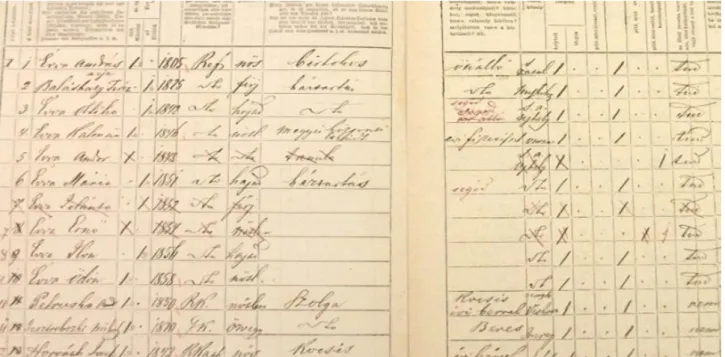
The census of 1870 was a specific one in the sense that the original household-level data sheets (figure 1) survived in some of the towns and villages, making it possible to carry out a more de- tailed inquiry compared to the officially published material, which aggregated data at settlement- level. Furthermore, the forthcoming censuses used personal datasheets instead of household-level inquiries, making it more difficult to carry out similar investigations to those published in this study. The original census sheets in 1870 contained the name, age, address, birth place, occupation and religion of the head of family, repeating these data for the wife, children, co-workers, servants and housemaids. It also provided the number of rooms, kitchens, economic buildings (stores, sta- bles, cellars) for each household. As the census did not contain income data, the mentioned varia- bles had to be used as proxies of wealth in order to classify population into social layers and to identify the elite. Beyond wealth general socio-demographic phenomena – either with or without spatial pattern (like the average children number of different occupation groups, average children number of different religions, migration patterns, mixed marriages, territorial aspects of marriage patterns, territorial distribution of religions etc.) – were also possible to trace using the mentioned variables.1 The data also offered possibility to create new variables beyond those given in the cen- sus, like population density (room/person), which was also used up as a proxy variable to meas- ure welfare.
Figure 1. Pages from the census, Nagy Piac str., nr. 9. Source:MNL-BAZML SFL XV. 83. box 77–79.
1 Demeter, G.-Bagdi, R.:A társadalom differenciáltságának és térbeli szerveződésének vizsgálata Sátoraljaújhelyen 1870-ben. (A GIS lehe- tőségei a történeti kutatásokban). Debrecen, 2016. (Investigating the Social Differentiation and Spatial Pattern of Society in Sátoraljaúj- hely, 1870. Applying GIS in Historical researches – in Hungarian).
The research was supported by the Hungarian Research Fund K 111 766.
III. The place
The selection of Sátoraljaújhely (the county seat of Zemplén County) as a sample area was ideal from several aspects. Not only the origial census sheets were available for 2150 households (10 000 inhabitants) offering substantial material for quantitative statistical analysis, but the timing itself was also fortunate.
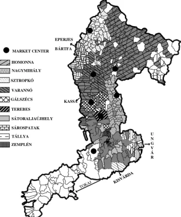
The town was located along the market line, where the products of the plains and mountains were exchanged. The physical geographical conditions allowed a N-S migration from the peripheries of Zemplén County to the county seat, while in the southern part of the county an E-W migration route developed towards the capital. Although in 1775 the county seat was unable to extend its attraction zone even to its own administrativ district (figure 2), between 1810-1870 its population has tripled, and this increase was among the greatest regarding their neighboring towns (table 1). By 1900 50% of the inhabitants of the county seat were born in a different locality, confirming the great role of migration.
The acceleration of urbanization processes made a melting pot from the town reflected in its religious diversity: 35% of the population was Jewish of origin, Roman catholics reached also 30%, Calvinist protestants 12-14%, Greek Catholics approximately 20%. As a basic step of industrialization the rail- way was opened in 1870, while guilds were dissolved in 1872, thus the parallel coexistence of tradi- tional and modern social patterns and layers are also observable owing to the date of conscription.
Table 1. Population increase referring to the rate of urbanization (1825–1900) in Sátoraljaújhely compared to the sur- rounding significant towns
Town Population increase Population in 1000 (1825) Population in 1000 (1900)
Eger 40 % 17.5 24.5
Kassa (Košice) 180 % 13 38
Miskolc 80 % 22 40
Sátoraljaújhely 200 % 4 (1784), 6.3 (1825) 10 (1870), 19.9 (1910) Beluszky P.: Magyarország településföldrajza. Általános rész. Budapest – Pécs, 1999.
HOMONNA NAGYMIHÁLY SZTROPKÓ
VARANNÓ GÁLSZÉCS TEREBES SÁTORALJAÚJHELY SÁROSPATAK TÁLLYA ZEMPLÉN
EPERJES BÁRTFA
KISVÁRDA KASSA
U N G V Á R
TOKAJ MARKET CENTER
Figure 2. Attraction zones based on market centers in Zemplén County in 1773.
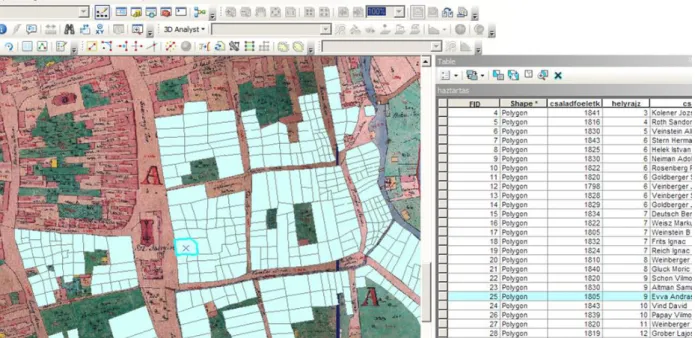
Figure 3. The basemap, the database containing the digitized census data, and the households-entities organized in GIS:
Nagy Piac str. nr. 9. Evva-household (nobleman)
IV. Methods
In order to carry out the investigations, raw census data were organized into a database containing the above mentioned variables, where each household represented an entity. Phenomena with spatial pattern were analysed using GIS (ArcGIS 10.1),2 while phenomena with no spatial rele- vance (within- and intergroup differences, like religious distribution within/between occupation groups, differences in welfare of religious groups and occupations, aging, differences in fertility rate, etc.) were evaluated using SPSS. The application of GIS required a map containing the same identifiers for households as the census data-sheets (topographical numbers), from the same era (1865) (figure 3).3
In case of welfare both spatial approach and the analysis of within and intergroup differences has relevance, thus both GIS and SPSS were utilized. The first step was to quantify welfare some- how. As social classifications are often not objective, we used 3 different methods to overcome so- cial prejudices. Besides the traditional classification based on the the prestige of occupation multi- variate statistics and SPSS were used for the other two classifications, both based on the quantified raw data of the census.
(1) In order to analyze patterns of traditional and modern layers of society we used Ferenc Er- dei’s model of ’accumulated society’, when classifying the cases into different social layers. This means, that besides the traditional elite, middle and lower classes; paralelly capitalistic formations evolved in each layer, and these were slowly fusioning by the 1910s.
(2) The second method to classify the inhabitants was based on an equation containing the room numbers, number of economic buildings, number of co-workers, number of servants and house- maids, and the number of household members as input variables. Thus, this classification focused on the per capita welfare, while the third one represented a classification, where the economic power of the household as an entity was cumulated. The intervals were set according to natural breaks, thus the groups did not have equal members.
2 A similar project led by Mazsu, János: OTKA 81488: The reconstruction of social and spatial pattern of Debrecen, 1870-72 was consid- ered the predescessor of this, but remained mostly unevaluated.
3 Source: MNL-BAZML SFL XV. 83. box. 77–79. Now www.hungaricana.hu and www.mapire.eu (containing settlement level cadastral maps) offers a new instrument to find detailed maps like this. The data sheets from Ung and Saros County are also left almost intact in county archives, thus there are plenty of options to repeat such investihgations
(3) The third method was based an automatic cluster analysis executed in SPSS containing the same variables except the number of family members. Classification results were checked by discrimi- nance analysis. After numerous attempts the number of clusters was finally set to 6, as above this value the proportion of successfully reclassified data began to drop, and the forming new groups remained small. Neither this classification produced groups of similar size.
It is not surprising that the three classifications did not have identical results (although there was strong correlation measured between the 3 classifications - over r=0.7 - and there was also strong correlation between the wealth categories and room numbers; wealth and population densi- ty/room), which is confirmed by cross-tabulations, correspondance analysis (table 2).
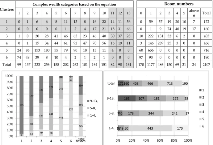
Table 2. Correspondence between complex wealth categories based on the equation and automatic clusterization
Clusters
Complex wealth categories based on the equation Room numbers
1 2 3 4 5 6 7 8 9 10 11 12 13 0 1 2 3 4 5 above
6 Total
1 0 1 6 6 8 11 13 8 16 22 14 11 56 0 59 57 19 20 10 7 172
2 0 0 0 0 0 1 2 4 17 21 18 31 66 0 1 9 74 40 19 17 160
3 1 0 20 28 41 46 63 23 46 40 30 37 28 10 222 131 32 6 2 0 403 4 0 1 15 34 44 61 92 47 70 56 16 19 11 3 146 289 25 3 0 0 466
5 24 86 153 180 55 79 90 18 13 11 4 0 0 60 656 0 0 0 0 0 716
6 74 49 39 8 10 4 2 1 2 1 0 0 0 97 93 0 0 0 0 0 190
Total 99 137 233 256 158 202 262 101 164 151 82 98 161 170 1177 486 150 69 31 24 2107
Figure 4. Correspondence of the 2 statistical evaluation (6 clusters, 13 groups based on equation)
The richest three groups (9-11) comprised 341 families (15%) in case of the 2nd method (equation referring to per capita economic power), while the richest 2 clusters comprised 332 family heads in the 3rd classification method, but only 192 were common of these (60%) (confirmed by figure 4).
V. Tracing the elite(s)
(1)Groups based on the traditional classification
The traditional (manual) classification based on the model of Erdei, Ferenc and Weber, Max result- ed in more than 10 categories with uneven size (table 3). Free civil professions and clerks were un- derrepresented here compared to other towns with similar functions. The layer of merchants was quite strong possibly as the result of Jewish abundance and the geographical location. The propor- tion of craftsmen was high, but not remarkably – the same was measured in the larger Debrecen.
Widows were separated as we have no information about their profession and incomes.
13 49 50
443 170
725 7
40
173 244 242
17
165 723 107
181 172
28 3
656
0%
10%
20%
30%
40%
50%
60%
70%
80%
90%
100%
1 2 3 4 5 6 összes
9-13, 5-8, 1-4,
total
0 7
165 172
13 40
107 160
49 173
181 403
50
244
172 466
443
242 28 713
170 17 190
0% 20% 40% 60% 80% 100%
1-4, 5-8, 9-13, total
1 2 3 4 5 6
The elite was composed of the ’f’, ’e’ and ’p’ categories, although as we will see, the wealth and economic power of the latter (civil professions) group was significantly weaker (teachers), than the other two according to data on room numbers, population density and the other two classification methods. Nevertheless, the categories do not strictly refer to welfare or social status: in category ’f’
smallholders and large estate owners are also included. But since they tended to live in the centre of the town, while agrarian wage-labourers (’s’) resided in the periphery, they were considered as part of the traditional (declining) elite.
The sectoral distribution of these categories is given in table 4. 35% of the family heads were in- volved in industry, but modern industrial branches were represented only by some 10% of the total family heads involved in industry – guilds still dominated referring to a transitional period.
The private tertiary reached 30% reflecting the transformations (urbanization), while agriculture has already lost its dominant position (25%). Those, who did not own or rent separate flats (or were not family heads), were omitted from the analysis (they ab ovo cannot be considered as mem- bers of elite), thus this table did not contain data on 1100 workers and 700 servants.4 In other words, only half of the wage-earners was included, thus percentage data on the elite below should be halved!
Table 3. Social groups according to the model of ’accumulated’ society (method 1; prs and %)
e town and county elite lawyers, chief clerks (state servants) 47 2.2%
f landowners mainly middle estate owners 116 5.4%
p free civil professions teachers, doctors, railway engineers, photographers, clockmaker 91 4.2 h clerks state (lower class compared to ’e’) and private (in banking and
finances) 108 5%
g agrarian experts not independent, but skilled agrarian wage-earners 34 1.6%
n policemen 29 1.5%
kk merchants mason owners, railway entrepreneurs, merchants 216 10.1%
k, ka lower officials: postmen, poor merchants 151 7.0%
m craftsmen guild members: tailors, potters etc. 677 31.5%
q lower tertiary transportation: cartsmen, waiters 60 2.8%
s poor daily wage earners in agriculture, beggars, bakers (women),
washerwomen, peripatetic, scrap-iron collector 508 23.7%
ö widows 101 4.7 %
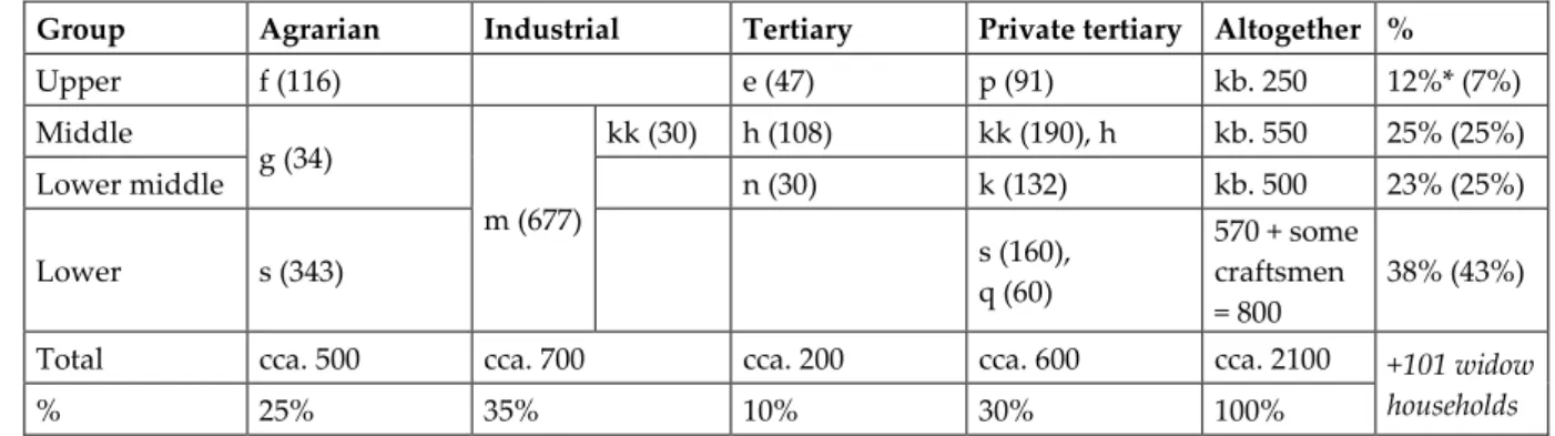
Table 4. Hypothetic-preconceptional social stratification based on the prestige of occupation (family heads; %) Group Agrarian Industrial Tertiary Private tertiary Altogether %
Upper f (116) e (47) p (91) kb. 250 12%* (7%)
Middle
g (34)
m (677)
kk (30) h (108) kk (190), h kb. 550 25% (25%)
Lower middle n (30) k (132) kb. 500 23% (25%)
Lower s (343) s (160),
q (60)
570 + some craftsmen
= 800
38% (43%)
Total cca. 500 cca. 700 cca. 200 cca. 600 cca. 2100 +101 widow
households
% 25% 35% 10% 30% 100%
*Servants or co-workers not conscripted as family heads were omitted. See corrected values including these layers in brackets.
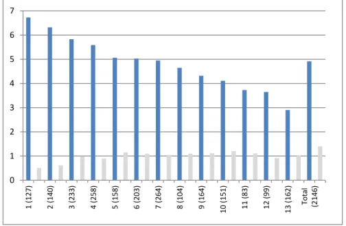
(2) Groups based on the welfare-equation
The family heads were classified into 13 groups based on the natural breaks in welfare values calculated by the equation. Groups 9-13 were definitely richer than the average. The richest 15% of
4 There were altogether more than 4000 persons conscripted with occupation, but only 2150 was family head.
families owned only 20% of the economic potential (it could reach 40% in Ottoman towns during the 18th c.).5 The next 20% owned 25% (figure 5), thus there were not significant differences within the elite. The poorest 20% owned only 13%. In other words the richer 50% of the population was 3 times richer, than the poorer half owning 25% of the economic potential. This inequality is not great measured to other regions. 6
Based on figure 5 the aggregation of wealth categories 11-13 (comprising 15% of households) may be reasonable. This is followed by group 9-10 including another 15% of the cases. (The reason of the small differences between these two groups might be, that members of the real elite had larger households, which decreased per capita economic potential. It is also true that within the 300 households there is a layer comprising 100 households with extremely high values).
Figure 5. The distribution of economic potencial (vertical axis) between groups of families (horizontal axis in %) The classification results confirm, that categories (based on the prestige of occupation) ’e’, ’f’,
’kk’, ’h’ are considered to be the richest, followed by ’p’, thus our preconception was not flawed (figure 6). The minor differences between the cluster-based and equation based classification (table 7) is due to the fact, that the latter measures total wealth of a family regardless of family size. Thus group ’f’ is considered poorer is per capita wealth is calculated as agriculture was labour-force intensive sector traditionally characterized by larger family size.
Figure 6. Differences in per capita economic potential between social groups based on prestige and occupation
5Canbakal, H.– Filiztekin, A.: Wealth and Inequality in Ott oman Lands in the Early Modern Period.Working Paper.
6 The richest 2% owned 25% in China, in New-Spain in 1790, the richest 10% owned 55% of the wealth, in Bihar (India) in 1804 the richest 20% owned 50%, and in Naples in 1811 it was 10 and 33% percent respectively. Milanovic, B–Lindert, P. H.–Williamson, J.
G.:Measuring Ancient Inequality. Working Paper 13550. NBER. Cambridge, MA, 2007. http://www.nber.org/papers/w13550.
0 5 10 15 20 25 30
7,50% 7,5-25% 25-45% 45-65% 65-85% 85-100%
0,5 1 1,5 2 2,5 3
Surpisingly the average room number/family was not higher than in rural areas (although the average household size – 4.66 prs – was bit smaller), the 1.5 room/family is not greater value than measured in Belgrade after 1900.7 Multistorey buildings were abundant only in the town centre, but even houses only with ground floor were usually divided between families (often not relatives). Only 12% of the households (not houses!) had more than 2 rooms – this can be the real elite as there was a strong correlation between room numbers and the calculated wealth based on the equation (table 5).
Further 22% had 2 rooms. Population density – calculated from room number and household size – is also an index of welfare (table 6). In 25% of households there were 4 or more than 4 inhabitants per room, while only 10% of families were characterized by density smaller than 1.5 person/room.
Table 5. Distribution of households based on room numbers in 1870 (prs and %) No data 0.5 room and
under 1 2 3 4 5 rooms
and above Total
40 170 1175 488 150 69 55 2147 (average: 1.5)
1.9 7.9 54.7 22.7 7.0 3.3 2.6 100 %
Table 6. Population density (prs/room) in Sátoraljaújhely in 1870 (prs and %)
under 1 1 1–1,5 1,6–2 2–2,5 2,5–3 3–4 above 4 Total
47 167 125 375 120 352 391 529 2147 (average: 2.85)
2.2 7.8 5.8 17.5 5.6 16.4 18.2 24.6 100 %
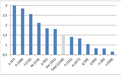
Table 7. The rankings of the pre-defined layers based on prestige of occupation using the two different statistical classification (cluster-based; equation-based)
e (47) h (108) f (116)
kk (214)
p
(91) ö (101) Total (2149)
k (132)
m (677)
g (34)
q (60)
n (30)
s (508) average
cluster membership
2.45 2.8 3.2 3.06 3.71 3.85 3.93 3.91 3.97 4.21 4.49 4.48 4.75
ranking 1 2 4 3 5 6 8 7 9 10 12 11 13
average equation- based wealth
4.52 2.85 2.57 2.12 1.84 1.81 1.49 1.41 1.33 1.04 0.83 0.82 0,66
ranking 1 2 3 4 5 6 7 8 9 10 11 12 13
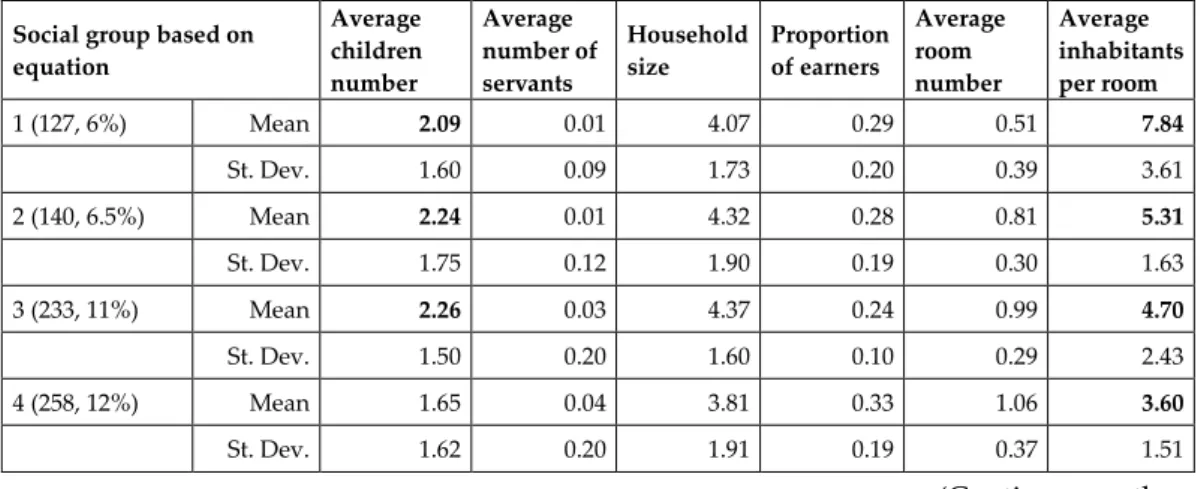
Table 8. Socio-demographic characteristics of the layers defined by the equation (the average represents intergroup differences, standard deviation represents within-group differences)
Social group based on equation
Average children number
Average number of servants
Household size
Proportion of earners
Average room number
Average inhabitants per room
1 (127, 6%) Mean 2.09 0.01 4.07 0.29 0.51 7.84
St. Dev. 1.60 0.09 1.73 0.20 0.39 3.61
2 (140, 6.5%) Mean 2.24 0.01 4.32 0.28 0.81 5.31
St. Dev. 1.75 0.12 1.90 0.19 0.30 1.63
3 (233, 11%) Mean 2.26 0.03 4.37 0.24 0.99 4.70
St. Dev. 1.50 0.20 1.60 0.10 0.29 2.43
4 (258, 12%) Mean 1.65 0.04 3.81 0.33 1.06 3.60
St. Dev. 1.62 0.20 1.91 0.19 0.37 1.51
(Continues on the next page)
7 In Belgrade in 1907 60% of the houses had only one room (as in the households of Sátoraljaújhely), but the density was 3.5 prs/house, while in the Hungarian town it was 9 prs (2 households/house). Vuksanović-Anić, D.: Urbanistički razvitak Beograda u periodu izmedu dva svetska rata (1919–1941). In: Istorija XX. veka. Zbornik radova IX. Beograd, 1968. 458–465. In 1926 an offcial or merchant family in Belgrade had 2.5 rooms, artisans had 1.9, workers had 1.5. The former values are similar to the Hungarian, while the latter are higher.
Calic, M-J.: Sozialgeschichte Serbiens 1815–1941. Der aufhaltsame Fortschritt während der Industrialisierung. München, 1994. 323-325.
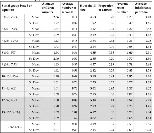
(Continues from the previous page) Social group based on equation
Average children number
Average number of servants
Household size
Proportion of earners
Average room number
Average inhabitants per room
5 (158, 7.5%) Mean 2.36 0.11 4.63 0.28 1.20 4.10
St. Dev. 1.77 0.32 1.92 0.16 0.49 1.65
6 (203, 9.5%) Mean 1.87 0.11 4.17 0.33 1.22 3.52
St. Dev. 1.89 0.33 2.19 0.15 0.49 1.62
7 (264, 12%) Mean 1.43 0.18 3.64 0.45 1.36 2.75
St. Dev. 1.73 0.40 2.24 0.30 0.58 1.64
8 (104, 5%) Mean 1.94 0.36 4.55 0.35 1.60 2.91
St. Dev. 2.00 0.59 2.55 0.20 0.77 1.50
9 (164, 7.5%) Mean 1.63 0.37 4.37 0.39 1.78 2.64
St. Dev. 1.62 0.59 2.42 0.25 0.83 1.58
10 (151, 7%) Mean 1.28 0.49 3.90 0.43 1.95 2.10
St. Dev. 1.61 0.70 2.33 0.27 0.77 1.39
11 (83, 4%) Mean 1.51 0.70 5.01 0.42 2.17 2.52
St. Dev. 1.69 0.79 2.95 0.30 1.07 1.65
12 (99, 4.5%) Mean 1.60 0.88 5.14 0.41 2.59 2.18
St. Dev. 1.70 0.97 2.99 0.29 1.28 1.45
13 (162, 7.5%) Mean 1.69 1.87 6.57 0.37 3.73 2.04
St. Dev. 1.89 1.62 3.87 0.26 1.66 1.64
Total (2149) Mean 1.81 0.34 4.39 0.35 1.53 3.50
St. Dev. 1.74 0.80 2.45 0.23 1.09 2.28
The narrow elite (group 11-13) was characterized by low children number, but with large family owing to the auxiliary workforce (table 8). The proportion of earners was higher than the city average, room number was over 2, as in group 9-10. The average population density was similar to that of group 9-10, because of the high number of servants (group 9-10 was characterized by smaller household sizes). Since the room number of the real elite was also similar to that of the middle class, it was the available auxiliary workforce that made real difference between them.
(3) Groups based on clusterization
Though the 3rd method to identify social strata was based on automathic classification, thus it lacked any preconception, unlike method 1 (prestige of occupation), the classification resulted in well-defined social characteristics (table 10), although the boundaries of some of the groups created were unconsolidated (group 2-3) as the discriminance analysis proved (table 9). Better classification results could not be achieved even when using less or more clusters.
Table 9. Discriminance analysis: successfully reclassed cases measured to total Original
cluster
Reclassed into Total case
number
1 2 3 4 5 6
1 123 8 0 40 1 0 172
2 21 10 30 53 34 12 160
3 0 11 270 17 94 11 403
4 1 1 16 353 95 1 467
5 0 0 0 0 716 0 716
6 0 0 2 6 71 111 190
Table 10. Socio-demographic characteristics of groups created by automatic clusterization Cluster 6: the poor, high children ratio, low proportion of earners, room number under 1 Cluster 5: the poor, no servants, small household size (3 prs!), room number around 1
Cluster 1: the rich, servant number over 2, low proportion of earners (0.2 – contrary to groups defined by the previous method, where it was over 0.4 – revealing that the two methods of defining the elite are not equivalent!), room number around 4
Cluster 2–3–4: average values, unconsolidated boundaries, fuzzy
Cluster 2: the proportion of Jews within the group is over 50%: ’par excellence Jewish middle- class’
The classification based on cluster membership was also appropriate to define groups based on their wealth as revealed by its combination with the classification based on the equation (figure 7), although the relation is not one-to-one. The average cluster membership of cases classified into equation-based groups 11-13 was under 3, while in the case of equation-based groups 1-6 it was above 5.
Figure 7. The average cluster membership of classes based on the equation
V.1. Socio-demographic features of the elite
The 170 households of the elite was characterized by high children number (over 2) contrary to the previous classification (with great standard deviation), but similarly to the high-middle class (cluster 2, 160 households) (table 8 and 11). The average number of servants was also around 2, while in cluster 2 it was under 1. The average household size exceeded 6.5 (with great standard deviation), which was remarkably higher than in cluster 2 or cluster 3-5, but similar to in group 13.
The proportion of earners was lower than in any other clusters, except cluster 6 (0.2 with low stan- dard deviation), and lower, than in group 13. Room number was 4, while it was only 2 in cluster 2 and 1 in cluster 5. Rich were averagely 5 years older (over 42 yrs), than measured in other clusters.
Population density was below 2 prs/room with low deviation (like in group 13), while it was over 3 in cluster 2 and over 7 in cluster 6. The average group membership in cluster 1 was above 11, while households classified into cluster 2 had a value over 9. Clusters 3-4 had average wealth based on the equation, while in the two categories comprising the poor the average group membership was only 4 and 2.
0 1 2 3 4 5 6 7
1 (127) 2 (140) 3 (233) 4 (258) 5 (158) 6 (203) 7 (264) 8 (104) 9 (164) 10 (151) 11 (83) 12 (99) 13 (162) Total (2146)
Table 11. Socio-demographic features based on automatic clusterization (average represents inter-group differences, standard deviation reveals within group differences)
Cluster (Ward- method)
Number of children
Number of servants
Household size
Proportion of earners
Average room number
Aging Prs/room
Group membership based on the equation Elite
(172)
Mean 2.30 1.97 6.61 0.22 3.97 1828 1.79 11.62
St. Dev. 2.07 1.48 3.33 0.15 1.46 12.62 0.97 1.64
2 (160) Mean 2.34 0.71 5.74 0.35 2.11 1832 3.29 9.54
St. Dev. 2.02 0.96 2.73 0.25 1.17 10.77 2.16 3.11
3 (403) Mean 2.26 0.21 5.51 0.43 1.54 1828.5 4.03 8.02
St. Dev. 1.70 0.46 2.39 0.22 0.76 11.21 1.82 2.90
4 (467) Mean 1.90 0.31 4.28 0.31 1.75 1829.6 2.71 7.58
St. Dev. 1.89 0.50 2.16 0.21 0.59 11.74 1.53 2.38
5 (716) Mean 1.06 0.00 2.91 0.38 0.96 1833 3.07 4.44
St. Dev. 1.07 0.00 1.21 0.24 0.14 12.00 1.19 2.04
6 (190) Mean 2.77 0.22 5.05 0.23 0.70 1833 7.84 2.34
St. Dev. 1.79 0.49 2.02 0.14 0.30 10.27 3.23 1.67
Total (2108)
Mean 1.83 0.34 4.42 0.35 1.55 1831 3.51 6.61
St. Dev. 1.74 0.80 2.45 0.23 1.08 11.77 2.28 3.46
As for the categories based on traditional classification (the weberian prestige of occupation), group ’e’ was characterized by more than 3 rooms, in case of group ’f’, ’h’ and ’kk’ it exceeded 2.
(Either owned or rented, room number represents economic power, figure 8).
Figure 8. Average room numbers per groups based on prestige of occupation
Figure 9. The connection between economic potential (based on the equation) and religion 0,0
0,5 1,0 1,5 2,0 2,5 3,0 3,5
,0 ,5 1,0 1,5 2,0 2,5 3,0
ev gk iz ort ref rk Total
Mean Std. Deviation
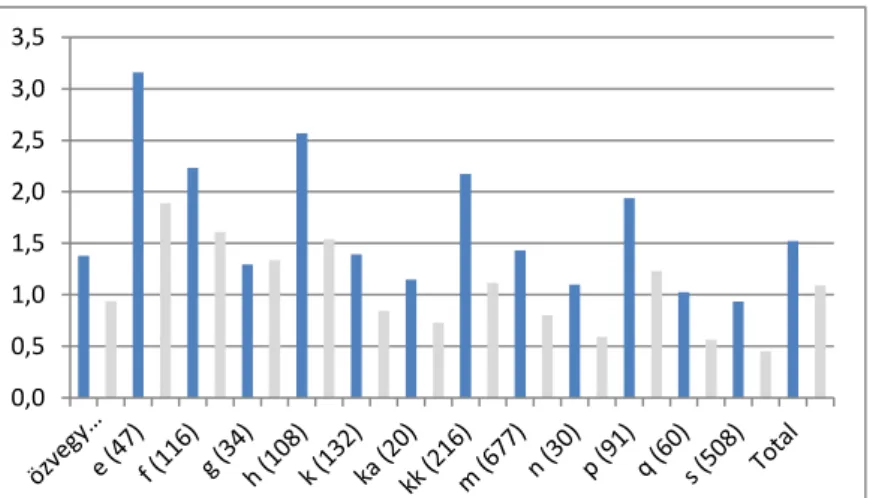
As for religious differences it was the Protestants (both Calvinists and Lutherans), whose economic potential proved to be the greatest followed by Jews (figure 9). Greek Catholics were poorer than the average. Although Calvinists constituted only 12% of the population they held traditionally most of the leading offices. Differentiation within religious groups progressed by 1870: standard deviation was high (there were poor artisans among Protestants, and beggars, scrap-metal collectors among Jews).
Internal differentiation
After analyzing the inter-group differences it is time to take a closer look on within-group differences earlier depicted by standard deviation values. Cluster 1 comprising the elite was dominated by group ’e’, ’kk’, ’h’ and ’f’ (’h’ and ’f’ constituted 20-20% of this group respectively referring to the predominance of old bureaucratic-agrarian classes, the new layer of merchants also reached 20% within cluster 1, but their proportion was still over 40% in the middle-class, cluster 2).
As these traditional categories based on the prestige of occupation can be found in other clusters as well, this confirms, that the 2 methods are not equivalent (figure 10). Only 50% of members in group ’e’ was classified into cluster 1, the chance to be the part of the elite was also 50% among ’h’
(officials), but only 15-15% in group ’kk’ and ’p’, while in group ’f’ 30% belonged to the elite. Al- most 30% of group ’kk’ was classified into cluster 2 (representing merchant burgeoisie). Thus it was category ’e’ and ’h’ that is considered dominantly the elite (these were officials referring to the fact that capitalist transformation was one-sided as new layers were not yet members of the high society here in 1870).
Figure 10. The classification of traditional groups into clusters: within-group differences 0%
10%
20%
30%
40%
50%
60%
70%
80%
90%
100%
ö e f h p kk k m g n q s Total
1 2 3 4 5 6
33
4
13 48
9 9 116
42
10 4
32 20
108 34
63
17
68
20 12
214 9
39
220
134
224 40
666
2 5
66 56
278 87
494
0%
10%
20%
30%
40%
50%
60%
70%
80%
90%
100%
1 2 3 4 5 6 összes
s q n g m k kk p h f e total ö
Surprisingly category ’p’ cannot be unequivocally considered as the component of the elite (only 10% of the elite stemmed from this category, though it is still higher, than their proportion from the total households, which is 5%; and only 15% of group ’p’ was classified as ’elite’ into cluster 1). This also refers to defects in modernization process of towns compared to the western models.
The above mentioned are also true if we use the equation-determined categories instead of automatic clusterization (figure 11). The proportion of cases classified into group 9-13 was over 70% in case of group ’e’ and ’h’, 50% in case of ’kk’ and ’f’, while 40% in group ’p’ (the agrarian elite was weakening, but the merchant elite was not yet strong to take over the positions of the bureaucrats – the agrarian elite transformed their power into political). As group 9-13 is a broader interval composed of more than 600 hundred families, while cluster 1 represented only 7.5% of the households (and cluster 2 gave further 7.5%), it is not surprising that artisans were also included into these aggregated groups.
Figure 11. Internal differentiation (based on economic potential) within traditional occupation groups
As for the religious distribution within the categories of theelitewe may conclude, that protestants were overrepresented within category ’h’ and Jews among members of group ’kk’
(both constituting the part of the elite), but within group ’e’ or group ’f’ no similar trends could be observed (figure 12); the share of different religions in the latter categories was similar to that of the total sample. The same phenomena can be observed if using the other two classifications.
Every family had 2 or more than 2 rooms (90% had more than 3) in cluster 1, while it was only 60% in cluster 2. 90% of family heads had 2 or more than 2 rooms in group ’e’, 60% in group ’f’, 70%
in group ’kk’ and ’h’, while it was only 40% among households classified into category ’p’ (figure 13).
0%
10%
20%
30%
40%
50%
60%
70%
80%
90%
100%
1-4, 5-8, 9-13,
0% 20% 40% 60% 80% 100%
1-4, 5-8, 9-13, Total
s q n m g k kk f p e h ö total
Going down into a deeper level we also tried to identify the proper occupations of the elite, within the pre-defined categories. Lawyers, doctors, engineers, landowners determined this group either we used averege room number, the equation to determine wealth or cluster analyis (table 12).
Figure 12. The frequency of different denominations among and within social groups based on prestige of occupation
Figure 13. The connection between room number and occupation 0%
10%
20%
30%
40%
50%
60%
70%
80%
90%
100%
ö e f h p kk k m g n q s Total
ev gk iz ref rk
18 100
155 120 283
676
2 184
102 40 179 507
0% 20% 40% 60% 80% 100%
ev gk iz ref rk összes
ö e f h p kk k m g n q s
0%
10%
20%
30%
40%
50%
60%
70%
80%
90%
100%
0,5 és alatta 1
2 3 4 4 felettover 4
Table 12. Rankings of different occupations based on their economic potential
Occupation of the family head
Average (category)
based on equation (14)
Ranking Cluster
(6) Ranking
Average room number
Ranking
Lawyers and doctors (33) 11.24 1 2.03 1 3.64 1
mason owners (60) 8.70 5 2.69 2 2.32 3
skinner-weaver (10) 9.40 2 3.10 3 2.9 2
landowners (106) 9.08 3 3.17 4 2.3 4
wheat, flour merchants (21) 6.76 14 3.33 5 1.81 9
engineers (18) 8.83 4 3.35 6
other merchants (38) 7.61 8 3.46 7 1.87 7
grocers (11) 6.82 12 3.55 8 1.55 12
joiner (35) 7.66 7 3.65 9 1.84 8
entrepreneurs, railway
entrepreneurs (13) 7.31 9 3.69 10 2.08 5
butchers (27) 6.89 11 3.74 11 1.56 11
small merchants (10) 6.10 18 3.78 12 1.00 26
textile merchants (15) 8.40 6 3.87 13 2.0 6
tanner-skinner (37) 6.57 15 3.89 14 1.27 18
woolen coat maker (aba) (46) 6.04 21 3.91 15 1.34 15
bootmakers (144) 6.11 17 3.92 16 1.33 16
total sample (2144) 6.53 16 3.93 17 1.52 13
shopkeekers (27) 5.52 23 3.96 18 1.19 21
shoemakers (16) 6.00 22 4.00 19 1.13 22
teachers (15) 6.80 13 4.07 20 1.77 10
tailors (103) 6.10 19 4.23 21 1.33 17
washers, sewers, bakers (37) 7.27 108 4.24 23 1.20 20
cartsmen (52) 4.83 25 4.55 24 1.00 24
carpenter (33) 4.61 26 4.73 25 1.11 23
personal servants (55) 5.00 24 4.73 26 1.00 25
agrarian daily wage earners (343) 3.89 27 4.88 27 0.87 27
policemen (15)9 3.73 28 5.00 28 0.86 28
V.2. Reproducing the elite
It is evident, that in urban environment natural reproduction was subordinated compared to migration as source of reproducing the elite. Even in the introverted Eger 75% of the measured population increase was the result of migration processes, as the net reproduction rate until 1873 was low (high mortality besides the high birth rate). The demographic transition in Hungary began only after the last cholera epidemics (1873).
External sources
As we mentioned, by 1900 55% of the urban dwellers in Sátoraljaújhely was born outside the administrative area of the town, which functioned as a ’sink’. The social distribution of the immigrant and indigenous society showed remarkable differences. High-class and upper classes were overrepresented among migrants compared to indigenous or total population, while the middle class was overrepresented in case of the indigenous population. Lower classes were also overrepresented among newcomers, especially regarding industrial-tertiary occupations, which clearly shows the changing workforce-demand of the transforming economy (table 13).
8 The differences in rankings using different classification method are due to the fact, that the equation calculates per capita potential contrary to the other two indices, thus a poor, but small family shows better performance when the equation is used as classification method.
9 Only heads of families included.
Table 13. Differences in social status of immigrant and indigenous society in Sátoraljaújhely (based on family heads)
Layers Total
number % Indigenous % Immigrant
%
Immigrants from the layer %
Examples
High class 50 2 13 1.5 2.1 74 priests, lawyers, doctors,
engineers High and upper
class 90 3.4 22 2.5 3.8 75
teachers, tax-collectors, railway engineers, local and county high- officials
Middle class 1080 41 435 50 36 60 merchants, craftsmen, mason
owners
Lower middle class 96 3.5 36 4.1 3.3 62 low-commission officers, grocers,
tailors, waiters
Lower classes 1390 52.5 341 39 58 75 nurses, servants, scrap-metal
and textile collectors Agrarian from
lower classes 558 21 183 21 21 67 peasants, daily labourers
Industrial- tertiary from lower classes
735 28 124 14 34 83 bricklayers, servants,
cartsmen, cooks
Altogether 2656 100 873 100 100 67
A regional comparison can also be useful to identify common and specific patterns. We analyzed the small Varannó oppid (Vranov, SK), a district center in the same county with only 2000 inhabitants, and the tradional, but introverted center, Eger (over 20 000), the county seat of Heves County (table 14). Not surprisingly the elite was mainly recruited from newcomers even in the small Varannó, as it had no school to educate its own elite. In the case of Eger, with its Lyceum, not only the elite was stronger regarding its percentage value compared to the other two settlements (20% vs. 3.5-7%) (although we used a different source type, the birth and marriage registers from 1883 containing only 870 persons and not the census data), but the local elite was also stronger compared to the immigrant elite society (22 vs. 12%). In Eger the middle class was thinner.
Table 14. A comparison of social stratification of immigrant and indigenous societies in urban and semi-urban environment
Layer Varannó total (%)
S.újhely, total (%)
Eger,*
total (%)
Varannó migrant (%)
S.újhely migrant (%)
Eger,*
migrant (%)
Varannó, indigenous (%)
S.ujhely, indigenous (%)
Eger,*
indigenous (%)
Elite 7.1 3.4 20.0 8.1 3.8 12.0 5.8 2.5 22.0
Middle 48.3 41.0 33.0 40.8 36.0 49.0 58.2 50.0 25.0
Lower
middle 6.1 3.5 24.0 8.6 3.3 12.0 2.9 5.0 28.0
Lower 38.5 52.0 22.0 42.5 58.0 25.0 33.1 39.0 20.0
Total
prs 720 2656 x 409
(57%)
1783
(67%) 311 (43%) 873 (33%)
*Eger is based on birth registers from 1883, while the other two were based on census data from 1870.
Internal sources
In order to analyze the chances of passing down or inheriting social positions, we used a sample of 100 persons (cca. 1% of the total population) between 1896 and 1906 collected from the birth registers of Sátoraljaújhely (narrow time interval was needed to identify father-son relations). In case of the elite both upward migration and the inheritance of social position was observable, but the sample was statistically irrelevant (table 15). The sum of cases predicts, that upward
movements were a bit more characteristic for this urbanising community than declassation (12 vs.
5 cases in 1896 out of 43; and 8 vs. 5 cases out of 40 in 1906, however stability characterized more than 50% of cases). As at least the sons were considered indigenous, thus the general improvement in their social status reveals the role of towns in ameliorating livelihood, while it is also evident, that in the society of (especially rural) immigrants lower classes dominated.
Table 15. Investigating social mobility in Sátoraljaújhely between 1896-1906 (father-son relations)
1896 cases
investigated
inherited
position % upward
movement % declassation %
Upper classes 2 1 50% 1 50% 0 0%
Middle class 34 17 50% 11 33% 3 9%
Lower classes 7 5 71% 0 0% 2 28%
1906
cases investigated
inherited
position %
upward
movement % declassation %
Upper classes 0 0 0% 0 0% 0 0%
Middle class 23 11 48% 8 34% 2 9%
Lower classes 17 9 53% 0 0% 3 18%
MNL-BAZML SFL, XXXIII-2. marriage registers from 1896, birth registers from 1906
V.3. Spatial pattern of the elite in different dimensions
After visualizing our data on maps, where each household was represented by an entity, we managed to locate the elite, which was characterized by a center-periphery accommodation pattern (Chart 1-5). Wealthy people were located along the main road in N-S direction (also representing the general route of migration), then in the city center, and the road leading towards the River Ronyva, perpendicular to the main road. The members of the elite often rented their houses in the city center to Jewish merchants, who there claimed the majority by 1870. As we used a multidimensional approach it is evident that the category of ’elite’ does not coincide in many cases after overlying the maps (wealth based on equation, clusterization, traditional classification, room numbers, density of dwellers).10
10 Contact with authors: Gábor Demeter (HAS, RCH, Institute of History), demetergg@gmail.com; Róbert Bagdi (Pallas Athena Univer- sity), bagdir@szolf.hu
Chart 1. Spatial pattern of population density (prs/room within households)
Chart 2. Spatial pattern of households (room / household)