1.Introduction GPU-ACCELERATEDSIMULATIONOFAROTARYVALVEBYTHEDIS-CRETEELEMENTMETHOD

(1)

hjic.mk.uni-pannon.hu DOI: 10.33927/hjic-2019-18

GPU-ACCELERATED SIMULATION OF A ROTARY VALVE BY THE DIS- CRETE ELEMENT METHOD

BALÁZSFÜVESI¹ ANDZSOLTULBERT^*1

1Department of Process Engineering, University of Pannonia, Egyetem u. 10, Veszprém, 8200, HUNGARY

The rotary valve is the most frequently used piece of equipment that is suitable for the controlled feeding or discharging of products in powdered or granular form. It is usually connected to silos, hoppers, pneumatic conveying systems, bag filters or cyclones. In this paper, a simulation study is presented on the discharge of solid particles from a silo through a rotary valve. The discrete element method (DEM), which accounts for collisions between particles and particle-wall collisions, was used to model and simulate the motion of individual particles. The diameter of the simulated silo was0.2m and a total of245,000particles were calculated. In the simulations, the effect of the geometric and operational parameters of the rotary valve on the mass outflow rate was investigated. The diameter of the rotary valve varied between0.06and 0.12m and the rotational speed of the rotor was changed between0.5and5s⁻¹. The simulations showed that the mass outflow rate of the particles from the rotary valve changes periodically due to its rotary cell structure. Within the lower range of rotational speeds of the rotor, the mass outflow rate of particles changes linearly in correlation with the rotational speed. The identification of this linear section is important in terms of control as this would facilitate the implementation of control devices by applying well-established linear control algorithms. Adjacent to the linear section, the dependence of the average mass outflow rate on the rotational speed was found to be nonlinear. Within the upper range of examined rotational speeds for each diameter of the rotary valve, the mass outflow rate reaches a maximum then decreases. The simulations were performed using GPU hardware. The application of parallel programming was an essential aspect of the simulations and significantly decreased the calculation time of simulations. In the treatment of particle-wall contacts, a novel flat triangular-based geometric representation technique was used which allows the particle-wall contacts to be calculated more effectively and their treatment implemented more easily into the parallel programming code. Using the calculated particle positions, the particles were visualized to view the effect of the interactions between the particles and rotor blades on particle motion. The simulation results showed that the discrete element method is capable of determining the detailed flow patterns of particles through the rotary valve at various rotational speeds.

Keywords: silo, rotary valve, simulation, discrete element method, GPU

1. Introduction

The handling of solids is part of many industrial tech- nologies in the chemical, pharmaceutical and food indus- tries amongst others. From simple storage (e.g. storage silo) and transport operations (e.g. pneumatic transport) to gas-solid or liquid-solid two-phase flows (e.g. gas- solid fluidization, gas-solid catalytic reactions), a number of technological operations involve solid and particulate materials. A common feature of gas-solid two-phase flow is that the interaction between the solid and gas phases can facilitate effective phase mixing in addition to intensive mass and heat transfer for a variety of operational purposes (e.g. gas-solid chemical reactions). The movement of the solid phase may result in different flow mechanisms and flow patterns, depending on the frequency of collisions between the particles and effects as a result of the gas stream. The experimental investigation of the unit

*Correspondence:ulbert@fmt.uni-pannon.hu

operations of particulate solids is time-consuming and costly. Measurements in this type of systems are often in- accurate due to the limitations of the measuring devices and difficulty of taking measurements in a solid flow without changing its flow properties. Although a number of advanced measurement techniques for measuring the flow properties of solids, e.g. phase doppler particle an- alyzer, high-speed video processing, magnetic resonance tomography, positron emission particle tracking, etc., ex- ist which provide useful information on the movement of particles, many factors that significantly influence the flow structure such as the forces between the colliding particles are not yet available.

However, experiments can be performed more easily using computer simulation if a sufficiently detailed model is available to investigate the system. The modeling and simulation of the flow of particulate solids are becom- ing increasingly popular and intensive research has been undertaken in this field. The flow of particulate solids is

(2)

always coupled with the flow of the interacting gas phase and in this sense the entire particulate flow can be con- sidered to be a gas-solid two-phase flow. However, the construction of the model depends on the degree of interaction between the solid and gas phases. The effect of the gas phase on the solid particles may vary from one unit operation to another. For example, in terms of the gravity discharge of solids from a silo, the effect of the gas phase is negligible on the motion of the particles and the calculation of any interaction between the solid particles and gas phase and the calculation of the gas phase flow are unnecessary. On the other hand, when pneumatic transportation is used to transport solids, the interaction between the two phases is significant, therefore, the modelling and calculation of flow characteristics of both the solid particles and gas phase as well as their interactions is necessary.

Two main methods for the treatment of solid particles with regard to gas-solid two-phase flows are proposed by the authors. The Euler method considers both the solid and fluid phases as a continuous phase and these methods are referred to as two-fluid models (TFM) in the literature. In these models, both phases are calculated by volume-averaged flow equations that are supplemented by terms which describe the interaction between the two phases. The disadvantage of these methods is that the solid particles are treated as a continuous phase and no information is provided about the motion of individual particles. In another method, the gas phase is treated as a continuous phase and described by volume-averaged flow equations, however, the solid particles are treated as discrete systems with their own mass, independent motion and velocity. The flow equations for the gas phase also in- clude terms that describe the interaction between the solid particles and the gas phase. To model and calculate the forces that result from particle-particle and particle-wall collisions, the discrete element method (DEM) based on the soft- or hard-collision model is used. These calculation methods are referred to as the Euler-Lagrange, Euler- discrete element method (EULER-DEM) or the Compu- tational Fluid Dynamics Discrete Element Method (CFD- DEM). If the effect of the gas phase on the particles is negligible, the motion of the particles can be calculated by applying the discrete element method alone without taking into account any interactions with the gas phase.

The discrete element methods have the advantage of pro- viding detailed information about the flow characteristics of solid particles. However, since all the particles are handled independently, they require significant computing capabilities in the case of a large number of particles.

In the application of “two-fluid” theory, Anderson and Jackson [1] first introduced interaction terms in the volume-averaged Navier-Stokes equation that is used to describe the particle-fluid and particle-particle interactions. In the 1990s, a significant amount of research using TFMs in the modeling and simulation of two-phase flow in fluidized beds was conducted by Bouillardet al. [2], Ding and Gidaspow [3], Kuiperset al.[4–6] and Nieuw-

landet al.[7]. McKeenet al.[8] simulated the movement of catalyst particles in a fluidized-bed catalytic cracking reactor. Wanget al.[9] developed a TFM including chemical reaction source terms that are capable of describ- ing homogeneous and heterogeneous reactions. Pougatch et al. [10] simulated particle attrition in a fluidized bed introducing an attrition term into the model. However, given the complexity of two-fluid models, they are un- able to describe the discrete particle dynamics and flow properties of individual particles.

The rapid development of computers and parallel computing over recent decades has led to the populariza- tion of discrete element methods in terms of the simulations of solid particulate flows and gas-solid two-phase flows. In the application of discrete element methods, the movement of each individual particle in the particulate flow is calculated. The motion of particles is calculated in accordance with Newton’s three laws of motion by taking into account the forces acting on the particles as a result of collisions with other particles or from their interactions with the gas phase.

Over the last two decades, numerous papers have been published regarding the application of the discrete element method. Tsuji et al. [11] and Kawaguchi et al.

[12,13] presented simulations of gas-solid fluidization by applying a soft collision model developed by Cundall and Strack [14]. In these simulations, the mixing of particles inside the fluidized bed was examined. Hoomans et al.

[15,16] used a hard-sphere collision model in their simulations and studied the effect of gas velocity on the flow of particles in a fluidized bed. Kanekoet al.[17] also used the CFD-DEM simulation method in the simulation of a polymer reactor. Using the temperature and velocity field of the gas phase, they calculated the kinetics of the poly- merization reaction and the reaction heat for each individual particle. Ulbertet al.[18] presented a CFD-DEM simulation study on the simulation of a reactive gas-solid two-phase flow in a circulating Mediator Recirculation Integrating Technology (MERIT) fluidized bed combus- tor. The model proposed by the authors contains the bal- ance equations for the components of the reaction and the shrinking core model was used to describe the gas- solid chemical reaction for each particle. Tsujiet al.[19]

presented a simulation study that calculated the motion of 4.5 million particles in a fluidized bed using parallel computation. Yanget al.[20] examined the effect of the surface energy of particles on the transitions between different flow types in a fluidized bed. Fanet al.[21] presented a simulation study on the simulation of cohesive particles. Accordingly, the cohesive surface interaction between the particles was taken into account when the interacting forces were calculated. Houet al.[22] simulated a fluid bed equipped with heat transfer tubes using the CFD-DEM simulation method. The authors examined the heat transfer between the tubes and the fluidized bed.

Houet al.[23] studied the effect of the particle-gas interaction, particle-particle collisions, gravity and friction on the transfer of energy between particles in particulate

(3)

Figure 1:Cross-sectional view of a silo equipped with a rotary valve.

solid flows and gas-solid two-phase flows.

As can be seen from the aforementioned examples, in addition to the calculation of the motion of discrete particles, the discrete element method is suitable to treat the discrete nature of the solid particle phase by taking into account further characteristics of discrete particles, e.g. temperature, concentration, etc.

The subject of this paper is the simulation of the operational characteristics of a rotary valve that is often connected to a silo that stores solids (Fig. 1). During the discharge of solids from silos, the effect of the gas phase on the movement of particles is negligible, i.e. it is unnecessary to consider the interaction between solid particles and the gas phase. Many examples are docu- mented in the relevant literature related to the simulation of discharging solids from silos using the discrete element method. Masson and Martinez [24] simulated silo feeding and discharge using the discrete element method.

In their simulation studies, the effect of the mechanical parameters of the particles on particle flow was studied. It has been shown that the friction and elasticity of the particles have a significant effect on the properties of particle flows. Yang and Hsiau [25] simulated silo feeding and discharge. In their research, different types of inserted elements were used and tested to improve the quality of the outflow of solid material from a silo. Goda and Ebert [26]

presented a simulation study that investigated the effect of particles on a wall using the discrete element method.

Gonzalez-Montellanoet al.[27] examined a laboratory- sized silo experimentally and by simulation to identify the coefficient of friction of the particles. Zenget al.[28]

examined the fluctuation in the velocity of the particles

being discharged from a silo. They showed that the velocity of particles fluctuates above a critical value of the coefficient of friction.

Few reports in the literature are related to experimental and simulation studies on rotary valves used to discharge or feed solids. A rotary valve connected to a silo was experimentally studied by Al-Din and Gunn [29].

The authors investigated the dependence of particulate mass flows delivered by the rotary valve on the rotational speed of the rotor and a linear relationship was found between the rotational speed and mass flow only within a certain range of rotational speed. Kirkwood et al. [30]

used a rotary valve to discharge solids from a silo and examined the mixing and segregation of solids inside the silo by analyzing the residence times. It was found that at low rotational speeds the particles segregated inside the silo and dead spaces developed in which the particles moved down significantly more slowly. However, at higher rotational speeds the entire particle bed of the silo moved evenly downwards, thereby ensuring that the solid layers that were fed into the silo did not mix.

The application of rotary valves occurs in all industrial areas where solids are stored in silos. The controlled discharge of the content of silos is important from both technological and control aspects. A deeper understand- ing of operational characteristics can significantly con- tribute to their geometric and operational design parameters. The simulation method used in our simulation study is the discrete element method, which provides a detailed insight into the flow of the solid phase inside a rotary valve. The purpose of the simulations is to determine how the geometric and operational design parameters of the rotary valve influence the mass outflow rate of solid material through the rotary valve.

The following chapters of this paper describe the discrete element method used in the modeling and simulation of particle flow, the triangular geometric representation technique used in the analysis of particle-wall collisions, the main features of the GPU hardware and parallel programming used in calculations, and the simulation results of the investigation of the effect of geometric and operational parameters of rotary valves on the mass outflow rate of solid particles.

2. Discrete element method

The discrete element method has become a popular method in the modeling and simulation of particulate flows. It is capable of calculating the motion of individual particles. The interactions between the particles and the boundary of the system are the collisions between particles and the particle-wall collisions which result in contact forces. The total contact force that acts on a single particle is the sum of the contact forces with regard to the forces that proceed from all the neighboring contacts. The individual particles exhibit two types of motion: translational and rotational. Translational motion is

(4)

caused by the contact forces and gravity. Rotational motion is generated only by the contact forces. In the case of when the effect of the gas phase is negligible, the three- dimensional translational and rotational motion of particles is expressed by Newton’s three laws of motion as follows:

m_ia_i=

j=q_i

X

j=1

(f_cn,ij+f_ct,ij) +m_ig, (1)

Iω˙i=

j=qi

X

j=1

(Tij+Mij), (2) whereq_idenotes the number of particles simultaneously in contact with particlei. m_i,a_i, andω˙_i are the mass, translational acceleration, and angular acceleration of particlei, respectively.f_cn,ijandf_ct,ijstand for the normal and tangential components of the contact force between particlesiandj,Tij is the torque at the point of contact between particles i andj due to the tangential contact force,Mij denotes the rolling resistance acting on particle i with regard to particle j,I represents the moment of inertia of particlei,gstands for the gravitational force vector, andri is a vector from the center of particleito the point of contact. The torqueTij is calculated using the tangential contact force by the vector cross product

T_ij=r_i×f_ct,ij. (3) The rolling resistanceMijis expressed by the following equation (Wensrich and Katterfeld [31]):

M_ij =−µr

r_ir_j ri+rj

|fcn,ij|(ω_ir_i−ω_jr_j), (4) whereµris the rolling resistance coefficient andriandrj

denote the radii of particlesiandj, respectively. When the particle collides with a wall,Eq. 4is simplified as

Mij=−µrri|fcn,ij|(ωiri). (5) After the contact forces and torque have been calculated, the translational and angular accelerations can be expressed fromEqs. 1and2 and the translational and angular velocities as well as position of particles can be calculated by numerical integration.

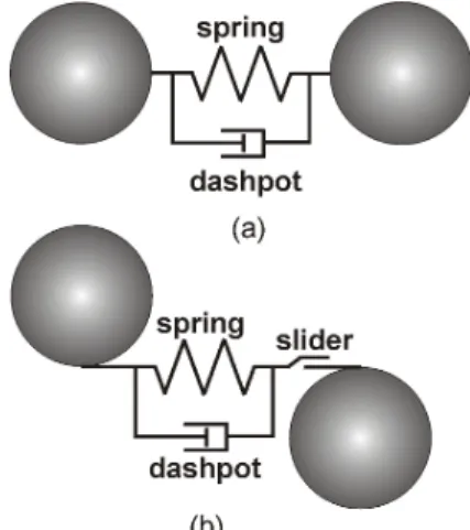
The calculation of contact forces can be divided into two groups, namely the calculation of normal and tangential contact forces. In our simulation, the contact forces were calculated in accordance with the soft-sphere contact model developed by Cundall and Strack [14]. In this model, the contact forces are calculated on the bases of simple mechanical models such as spring, dashpot and friction elements (Fig. 2 ). These mechanical elements influence particle motion through the parameters of the spring constantk, damping coefficientη and coefficient of frictionµ.

The sum of the normal forces is yielded by the normal forces generated by the spring and dashpot element:

fcn,ij = (−knδn,ij−ηnvr,ij·nij)nij. (6)

Figure 2:Soft-sphere contact model: (a) normal direction, (b) tangential direction.

Similarly, in the tangential direction, the sum of tangential forces acting on particleiis

f_ct,ij =−ktδ_t,ij−η_tv_rs,ij, (7) where vectorn_ijdenotes a unit vector from the center of particle i to the center of particlej,vr,ij represents the relative translational velocity of the colliding particles, δn,ijstands for the normal particle displacement,δt,ijis the tangential particle displacement vector andvrs,ijdenotes the relative slip velocity of the particles.

2.1 Calculation of the normal and tangential displacement of particles

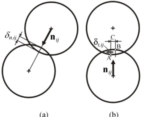
During elastic collisions between particles, at first particles are deformed and compressed, then expand and start to move in the opposite direction. This mechanism is modeled in the soft-sphere contact model by assuming the shape of particles is unchangeable. When two particles collide, they overlap with each other and the distance between their centers becomes smaller than the sum of their radii. Based on this overlapping, a normal displace- mentδn,ij, as shown inFig. 3, can be defined as

δn,ij= (di+dj)/2− |pi−pj|, (8) wherediandpiin addition todjandpjare the diameters and position vectors of particlesiandj, respectively.

The calculation of contact forces in the tangential direction is also based on a displacement defined in the tangential direction. As the particles first make contact, the points of impact A and B are the same points of the space (Fig. 3). The location of two points is continuously changing due to the translational and rotational motion of particles and a distance (C) between the two points evolves which is equal to the absolute value of the tangential displacement vector δt,ij. The direction ofδt,ij

is perpendicular to the unit vectornij and extends from the actual point of contact. As the collision proceeds, the absolute value and direction of the displacement vector

(5)

Figure 3:Illustration of normal and tangential particle displacement.

change according to the instantaneous relative slip velocity at the point of contact. Moreover, the directions of the unit vectornij and tangential displacement vectorδt,ij

also change in accordance with the translational movement of particles during the collision (Fig. 4). For this reason, the value of the tangential displacement vector is corrected by two steps. At first, the original value of the tangential displacement vector is transformed into the new position of particles defined by the unit vectorn_ij. In the second step, the transformed tangential displacement vector is corrected by the time integration of the relative slip velocity.

2.2 Calculation of the slip velocity

The tangential component of the relative translational ve- locityvrt,ijcan be determined as

vrt,ij =vr,ij−(vr,ij·nij)nij, (9) wherevr,ij = vp,i−vp,j is the relative translational velocity. The circumferential velocityvc at the point of contact is calculated by the angular velocityωof the particles. For particlei, it is given as

vc,i= (|ri|ωi)×nij. (10) By using the circumferential velocities, the relative slip velocity can be determined from

v_rs,ij= (v_c,i−v_c,j) +v_rt,ij. (11)

2.3 Calculation of the slide of particles

When two particles come into contact, the normal force fcn,ij presses them together. The sliding motion of surfaces introduces a tangential force of friction that acts on the surface in the direction which opposes the motion.

In our simulations, the Coulomb’s law of friction is applied to calculate the slide of particles. The magnitude of the tangential contact force vector is verified against the value ofµ|fcn,ji|, where µrepresents the coefficient of friction between particlesiandj. If the absolute value of

Figure 4:Change in particle orientation during the collision.

fct,ijexceeds that ofµ|fcn,ji|, the particles slide and the value of the tangential contact force is changed in accordance with

f_ct,ij=µ|fcn,ij|t_ij, (12) wheretij =fct,ij/|fct,ij|defines a unit vector. When the particles slide, the tangential contact forcefct,ij is con- sidered to be exerted only by the spring. Therefore, a new value of tangential displacement vector δt,ij, which is identical to the new value of the tangential contact force, must be calculated:

δt,ij= µ|fcn,ij| k

δij

|δ_ij|. (13)

2.4 Calculation of the damping coefficient

The damping coefficientηof a dashpot can be related to the coefficient of restitutioneaccording to

η=−2√

mk lne

q

π²+ (lne)²

(14)

developed by analytically solving the equation that de- scribes a damped oscillatory system containing a mass, spring and dashpot (Tsujiet al.[11]).

2.5 Treatment of particle-wall collisions

Particle-wall contacts can be deduced from particle- particle contacts. On the external side of the wall the particle comes into contact with, a mirror particle is placed with an angular velocity of zero (Fig. 5). The unit vector n_ij, from the center of particleito the center of mirror particlej, is always perpendicular to the wall plane. In the case of a motionless wall, the translational velocity of a mirror particle is zero. Consequently, the relative velocity between the contacting and mirror particles is the same as the velocity of the contacting particle. When the particle comes into contact with a moving wall, the translational velocity of the mirror particle is identical to the velocity of the point of impact. Under these conditions, the contact forces for particleican be calculated in a similar way to in the case of particle-particle contacts.

(6)

Figure 5: The placement of a mirror particle during a particle-wall collision.

3. Conditions of simulation

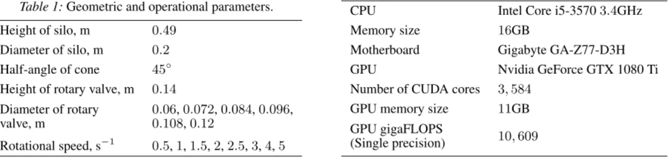
Simulation of the three-dimensional motion of particles was conducted in a silo equipped with a rotary valve as shown inFig. 1. The dimensions of the silo and rotary valve are given inTable 1. The number of spherical particles of uniform size used in the simulation study was 245,000. The particle properties used in the simulation are summarized inTable 2. The initial particle bed com- pletely filled the silo above the rotary valve as shown in Fig. 1.

In the simulation study, the effect of the geometric design and operational parameters of the rotary valve on the mass outflow rate was examined. In total48simulation runs were accomplished. The diameter of the rotary valve varied between0.06and0.12m. The rotational speed of the rotor was adjusted between0.5 and5 s⁻¹. The parameters of the simulation runs are summarized inTable 3.

The specifications of the computer and GPU used in the simulation study are shown inTable 4.

4. Geometric representation of the silo and rotary valve

During the discharge of the silo through the rotary valve, particles come into contact with each other and the walls.

The walls of the silo are stationary, on the other hand, in the case of the rotary valve, the walls of the body are stationary and the walls of the rotating rotor move.

The detection and treatment of particle-wall collisions require the calculation of the distance between the particle and wall which is based on the normal vector of the

Table 1:Geometric and operational parameters.

Height of silo, m 0.49 Diameter of silo, m 0.2 Half-angle of cone 45^◦ Height of rotary valve, m 0.14 Diameter of rotary

valve, m

0.06,0.072,0.084,0.096, 0.108,0.12

Rotational speed, s⁻¹ 0.5,1,1.5,2,2.5,3,4,5

Table 2:Particle properties used in the simulations.

Diameter, m 0.004

Density, kg/m³ 1190

Spring constant, normal direction, N/m 800 Spring constant, tangential direction, N/m 800 Coefficient of restitution,e 0.6

Friction coefficient,µ 0.43

Rolling resistance coefficient,µr 10⁻⁴

Table 3:Parameters of simulation runs.

Number of particles 245,000

Simulation time, s 4

Timestep, s 5×10⁻⁵

Interval for data saving, s 0.002 Number of standing wall elements 500−600 Number of moving wall elements 24

wall surface. In the case of flat walls, the normal vector can be determined easily. However, in the case of curved surfaces, the calculation of the normal vector of the surface and contact point is much more computation- ally complex. The number of calculations can also be increased significantly when collisions with moving walls are taken into consideration.

Therefore, in our simulation technique, the equipment walls are approached in accordance with a set of flat triangles which allows wall collisions to be detected and contact forces to be easily calculated. This has two advan- tages over the conventional treatment of particle-wall collisions using the mathematical definition of curved surfaces. On the one hand, any curvature wall can be easily defined by a set of flat triangles using methods developed in the field of computer graphics. The surfaces and ge- ometries created using computer graphics software can be saved and imported into the simulation program along with the other simulation parameters. As a result, the geometry of the equipment can be altered in the program without changing the programming code. In the case of the application of moving walls, the description of the movement of the triangles is also produced by computer graphics software and imported into the simulation program.

Another advantage is that the GPU can work more

Table 4:Details of the computer hardware.

CPU Intel Core i5-35703.4GHz

Memory size 16GB

Motherboard Gigabyte GA-Z77-D3H

GPU Nvidia GeForce GTX 1080 Ti

Number of CUDA cores 3,584

GPU memory size 11GB

GPU gigaFLOPS

(Single precision) 10,609

(7)

Figure 6:The flat triangular approximation of the silo geometry.

efficiently if the threads need to conduct similar calculations simultaneously. Thus, it is advantageous for the GPU to process the treatment of many triangles of the same structure as opposed to just a few but different structures of equations for the surface. A further advantage of the flat triangular approximation is that its accuracy can be increased where required by using more triangles, e.g.

the approximation of the silo geometry by a set of flat triangles is shown inFig. 6.

In the treatment of particle-wall collisions, it is necessary to determine the position of mirror particles. When using the flat triangular approximation, firstly it is necessary to check whether the given particle can collide with the given triangle. If the particle collides, the point of the triangle closest to the particle is determined using the method developed by Mark W. Jones [32]. Then the position of the particle is mirrored on the opposite side of the triangle in the direction given by the normal vector.

5. Application of the GPU

To apply the discrete element method effectively, the computer hardware used for the calculations has to be capable of parallel computing the motion of individual particles. In our simulation study, GPU cores and parallel programming were used to calculate the particles in parallel. A GPU core was assigned to each particle. A core can only write data in the memory associated with the particle but can read all the data from the memory associated with the other particles to analyze collisions between particles. As a consequence, all the data that results from the calculation of a collision between two particles is stored in two memory places. This solution had to be applied to avoid problems related to the writing of dupli- cates. Additionally, because of the way data is read, associated problems may arise when new data is calculated

from the data in both the previous and current iterations.

To overcome these problems, two data units were used, one always contained the data of the previous iteration and the other stored that of the current iteration.

The number of particles simulated may exceed the number of cores in the GPU, therefore, particles are calculated in consecutive batches. After calculating a batch of particles assigned to the GPU cores, a new group of particles is added to the GPU cores and they are calculated. This process is repeated until each particle has been calculated, then the next iteration is executed.

It is also important to note that during the parallel ex- ecution all the calculation data is stored in the memory of the GPU and that the CPU only gives instructions to the GPU about which calculations to perform. Therefore, at the beginning of the simulation, all the initial data con- cerning particles and walls are copied into the memory of the GPU and the CPU is used to instruct the GPU to perform the calculations. Since the copying of data between the memories of the GPU and computer (host) is slow, this would increase the run time of the program, so it is important that the copying of data between the two memories is limited. For this reason, two computational cycles were defined. During the internal cycle, only the GPU is working, it executes a defined number of iterations. At the end of the internal cycle, control is passed on to the external cycle and the data is copied to the host memory and saved as a file.

It is also important to note that executing the code on the GPU is effective if all the GPU cores conduct the same calculation. Attention should be paid to the use of branch instructions as they can significantly impair performance.

6. Simulation results and discussion

In the aforementioned simulations, the startup process of silo discharge and the effects of the diameter of the rotary valve and rotational speed of the rotor on the mass outflow rate of particles leaving the rotary valve were investigated.

6.1 The startup process of silo discharge

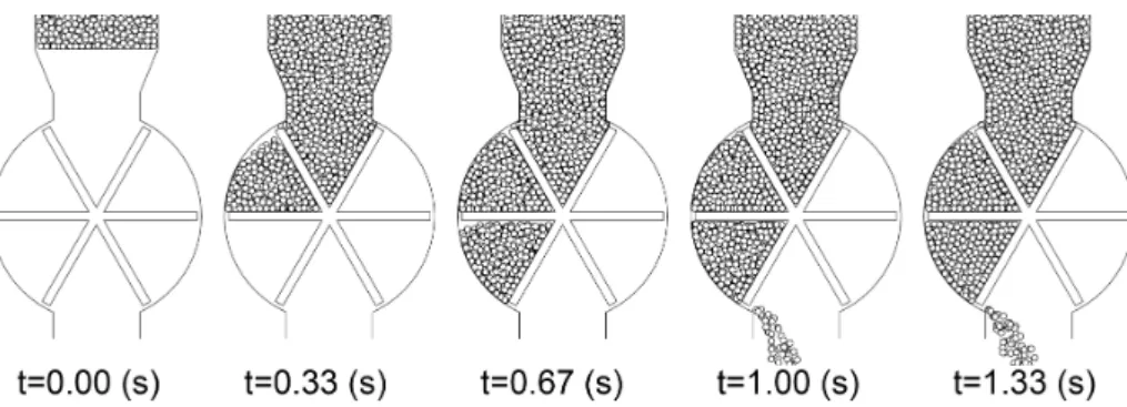
The startup process of silo discharge through the rotary valve is shown in a cross-sectional view in Figs. 7 and 8at different rotational speeds.Fig. 7shows the startup process at a rotational speed of0.5s⁻¹. The positions of the particles were visualized six times per revolution. At this rotational speed, the particles have sufficient time to fill the entire volume of the cell. Particles entering the cell are forced to pass by the blades of the rotor. When a cell reaches the outlet, all the particles fall out of the cell.Fig.

8 shows the startup process of discharge at a rotational speed of5s⁻¹. In this case, the blades of the rotor rotate so fast that the particles do not have sufficient time to fill the entire volume of the cell. Approximately only one third of the volume of the cell is filled with particles. The

(8)

Figure 7:The startup process of silo discharge at a rotational speed of0.5s⁻¹.

blades push the particles so strongly that they collide with the wall of the outlet channel and accumulate. As a result, not all the particles are capable of falling out of the cell and some remain in the rotary valve.

6.2 Analysis of the mass outflow rate through the rotary valve

During silo discharge through a rotary valve, the mass outflow rate exhibits a pulsating, periodic change over time as a consequence of the rotating cellular structure of the rotary valve. Following a finite period of time after the rotary valve starts to operate, a periodic change in the outflow of particles develops of constant amplitude and frequency. Depending on the geometric and operational parameters, the amplitude and frequency of this periodic change may vary.

To compare the effect of the various geometric and operational parameters on the mass outflow rate, it is necessary to calculate the time-averaged pulsating mass out-

flow rate. Therefore, the simulation time was sufficient to obtain at least ten cycles of change of constant amplitude and frequency. The time-averaged mass outflow rate was calculated from the simulation data saved after certain in- tervals of time.

First, the number of particles discharged from the silo during the time interval between data saves was determined. Next, the resulting data was multiplied by the volume and density of the particles and divided by the time interval between data saves to obtain the periodic time variation of the mass outflow rate. Finally, the time- averaged mass outflow rate was obtained by averaging the values throughout the simulation.

For example,Figs. 9and10show the dynamic change in the mass outflow rate of particles at rotational speeds of 0.5 and5s⁻¹when the diameter of the rotary valve was0.12m. When the rotational speed was5s⁻¹, only the initial part of the entire simulation observed a high- frequency periodic change in the mass outflow rate more clearly. By comparing the two figures, it can be seen that

Figure 8:The startup process of silo discharge at a rotational speed of5s⁻¹.

(9)

Figure 9:The dynamic change in the mass outflow rate at a rotational speed of0.5s⁻¹.

as the rotational speed increases, a periodic change of higher frequency and smaller amplitude was observed.

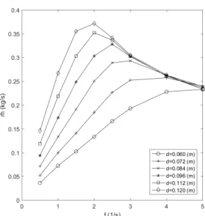
Fig. 11 shows the dependence of the time-averaged mass outflow rate on the rotational speed of the rotor when the diameter of the rotary valve was varied. The curves represent different diameters of the rotary valve.

It can be observed that as the diameter increases, the average mass outflow rate rises. In the first section of the curves, the mass outflow rate increases linearly as the rotational speed of the rotor rises. This section is significant in terms of its control. Linear industrial controllers are well established and suitable for the application of control theory for linear systems. The linear control theory ap- plies to systems whose output is proportional to their in- put. These types of systems are governed by simple linear differential equations, while nonlinear systems are often governed by nonlinear differential equations and mathematical techniques developed to handle them are much more complex and far less general. Due to the linear dependence of these sections, the mass outflow rate can be easily controlled by common industrial control systems

Figure 10:The dynamic change in the mass outflow rate at a rotational speed of5s⁻¹.

Figure 11: The dependence of the rotational speed on the time-averaged mass outflow rate using different rotary valve diameters.

based on linear control algorithms. InFig. 11, it can also be observed that the length of linear sections depends on the diameter of the rotary valve.

The linear section in the case of the smallest diameter of 0.06m occurs between rotational speeds of 0.5−3 s⁻¹, while in the case of the largest diameter of0.12m it occurs between rotational speeds of0.5−1.5s⁻¹. Since a desired mass outflow rate can be more easily controlled in a linear section with a smaller gradient, it is advisable to keep the diameter as small as possible.

Following the initial linear section, the mass outflow rate reaches a maximum value, the larger the diameter, the greater the maximum value of the mass outflow rate.

If a mass outflow rate in excess of the maximum value is required, this can only be achieved by increasing the diameter and not by raising the rotational speed. As the diameter of the rotary valve decreases, the rotational speed at which the maximum is observed increases, as shown in Fig. 11. After the maximum is achieved, a decreasing section follows where the time-averaged mass outflow rate begins to decrease. Since the location of the maximum shifts towards higher rotational speeds as the diameter of the rotary valve increases, the decreasing section also shifts. Between the rotational speeds of4and5s⁻¹, the mass outflow rates for each diameter converge.

The optimal value of the diameter of the rotary valve can be determined based on the length of the linear section. A given mass outflow rate can only be achieved with a sufficiently large diameter. However, the use of a larger diameter is not recommended as the gradient of the linear range increases as the diameter increases and control of the system becomes less precise. By considering the range beyond the maximum, it is clearly unnecessary to operate a rotary valve of a given diameter at higher rota-

(10)

Figure 12:The flow patterns of particulate flows at different rotational speeds of the rotor.

tional speeds to increase the level of performance, since the maximum mass outflow rate cannot be exceeded, in fact it may even decrease.

6.3 Flow patterns of the particles at different rotational speeds of the rotor

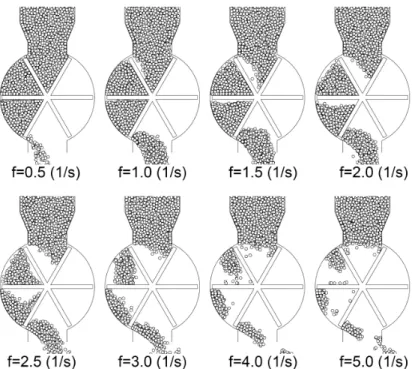
As was shown inFigs. 9and10, the mass outflow rate exhibits a constant periodic change after the startup process of discharge. In order to understand the phenomena that occur inside the rotary valve with a greater degree of accuracy, the positions of the particles were visualized to obtain the instantaneous particle flow patterns visible at various rotational speeds of the rotor (Fig. 12).

In all cases, a cross-sectional view of the rotary valve is presented when the rotor blades were in the same position and the operation was already within the range of the constant periodic change.Fig. 12shows the gradual decrease in the charge of cells as the rotational speed increases. At a rotational speed of0.5 s⁻¹, the cells still have sufficient time to fully recharge. Between rotational speeds of1.0 to1.5 s⁻¹, an empty volume fraction re- mains in the cells after being charged. At these rotational speeds, this empty volume fraction is still small and the accelerated feed and discharge periods can compensate for the decreasing mass outflow rate. At a rotational speed of2s⁻¹, the time-averaged mass outflow rate reaches its maximum. When the rotational speed was2.5s⁻¹, the resulting empty volume fraction of the cells becomes even bigger but the particles rest on the lower blade. At a rotational speed of3 s⁻¹ a significant change can be observed in the operation. At this rotational speed, the particles seem to float between the blades of the cell, i.e. the

speed of the blades is equal to the rate at which the particles drop. At a rotational speed of4 s⁻¹, the particles are already pushed forward by the top blades. By further increasing the rotational speed (5s⁻¹), the time the cells have to be recharged is so small that the mass outflow rate begins to decrease even more.

7. Conclusions

Generally speaking, it can be said that by using the discrete element method in particulate flow simulations, it is possible to observe particle flows in detail and to bet- ter understand related phenomena. The simulation study presented in this paper focused on the simulation of the discharge of solid particles from a silo controlled by a rotary valve using the discrete element method. In the simulations, the mass outflow rate of particles was ana- lyzed along with different geometric and operational parameters of the rotary valve. By applying the discrete element method, it was possible to dynamically simulate the movement of individual solid particles through the rotary valve and examine the mass outflow rate of particles.

By visualizing the individual particles at their positions, the effect of the interaction between the particles and the blades of the rotary valve on the flow patterns of particles at different rotational speeds was observed.

The simulations showed that the mass outflow rate of the particles leaving the silo changes periodically due to the rotating cell structure of the rotary valve. The dependence of the time-averaged mass outflow rate on the rotational speed of the rotary valve was found to be nonlinear within the upper range of examined rotational speeds.

However, for each diameter of the rotary valve, a range of rotational speeds in which the mass outflow rate changes

(11)

linearly with the rotational speed was observed. Within these ranges of linear speed, the rotary valve can be used more advantageously to perform different control tasks.

Following the linear range, for each diameter of the rotary valve, the mass outflow rate reaches a maximum then decreases.

The simulations were performed using GPU hardware. The application of parallel programming is an essential part of the simulations and can significantly decrease the calculation time of simulations from a few days to just a few hours. By considering the treatment of particle-wall contacts, a novel flat triangular-based geometric representation technique was proposed which also made it possible to calculate the particle-wall contacts in parallel by GPU.

Symbols

p position vector of a particle, m v velocity vector of a particle, m/s a acceleration vector of a particle, m/s² g gravitational acceleration vector, m/s² f force vector, N

T torque vector, Nm

I moment of inertia of a particle, kgm² d diameter of a particle, m

r radius of a particle, m

e coefficient of restitution, dimensionless k spring constant, N/m

m mass of a particle, kg n unit vector, dimensionless t unit vector, dimensionless Greek letters

δ normal displacement, m

δ tangential displacement vector, m η damping coefficient, kg/s

µ coefficient of friction, dimensionless

µr coefficient of rolling resistance, dimensionless ρ density of a particle, kg/m³

ω angular velocity vector, s⁻¹ Subscripts

c circumferential cn normal contact ct tangential contact

n normal direction, normal component r relative

rt relative tangential rs relative slip

t tangential direction, tangential component

Acknowledgement

This research was supported by the State of Hun- gary within the framework of the project 20385- 3/2018/FEKUSTRAT.

REFERENCES

[1] Anderson, T.B., Jackson, R.: A fluid mechanical description of fluidized beds.I&EC Fundamentals 1967,6(4), 527–539DOI: 10.1021/i160024a007

[2] Bouillard, J.X., Lyczkowski, R.W., Gidaspow, D.:

Porosity distribution in a fluidized bed with an im- mersed obstacle. AIChE J. 1989, 35(6), 908–922

DOI: 10.1002/aic.690350604

[3] Ding, J., Gidaspow, D.: A bubbling fluidization model using kinetic theory of granular flow.AIChE J. 1990,36(4), 523–538DOI: 10.1002/aic.690360404

[4] Kuipers, J.A.M., Prins, W., van Swaaij, W.P.M.:

Theoretical and experimental bubble formation at a single orifice in a two-dimensional gas-fluidized bed.Chem. Eng. Sci.1991,46(11), 2881–2894DOI:

10.1016/0009-2509(91)85157-S

[5] Kuipers, J.A.M., van Duin, K.J., van Beckum, F.P.H., van Swaaij, W.P.M.: A numerical model of gas-fluidized beds. Chem. Eng. Sci. 1992, 47(8), 1913–1924DOI: 10.1016/0009-2509(92)80309-Z

[6] Kuipers, J.A.M., van Duin, K.J., van Beckum, F.P.H., van Swaaij, W.P.M.: Computer simulation of the hydrodynamics of a two-dimensional gas- fluidized bed. Comput. Chem. Eng. 1993, 17(8), 839–858DOI: 10.1016/0098-1354(93)80067-W

[7] Nieuwland, J.J., Veenendaal, M.L., Kuipers, J.A.M., van Swaaij, W.P.M.: Bubble formation at a single orifice gas-fluidized beds. Chem. Eng.

Sci. 1996, 51(17), 4087–4102 DOI: 10.1016/0009- 2509(96)00260-6

[8] McKeen, T., Pugsley, T.: Simulation and experimental validation of a freely bubbling bed of FCC catalyst.Powder Technology2003,129(1–3), 139–

152DOI: 10.1016/S0032-5910(02)00294-2

[9] Wang, X., Jin, B., Zhong, W.: Three-dimensional simulation of fluidized bed coal gasification.Chem.

Eng. Proc.: Proc. Int. 2009, 48(2), 695–705 DOI:

10.1016/j.cep.2008.08.006

[10] Pougatch, K., Salcudean, M., McMillan, J.: Simu- lation of particle attrition by supersonic gas jets in fluidized beds.Chem. Eng. Sci. 2010,65(16), 4829–

4843DOI: 10.1016/j.ces.2010.05.031

[11] Tsuji, Y., Kawaguchi, T., Tanaka, T.: Discrete particle simulation of two-dimensional fluidized bed. Powder Technology 1993, 77, 79–87 DOI:

10.1016/0032-5910(93)85010-7

[12] Kawaguchi, T., Tanaka, T., Tsuji, Y.: Numerical simulation of two-dimensional fluidized beds using the discrete element method (comparison between the two- and three-dimensional models). Powder Technology 1998, 96, 129–138 DOI: 10.1016/S0032- 5910(97)03366-4

[13] Kawaguchi, T., Sakamoto, M., Tanaka, T., Tsuji, Y.:

Quasi three-dimensional numerical simulation of spouted beds in cylinder.Powder Technology2000, 109, 3–12DOI: 10.1016/S0032-5910(99)00222-3

(12)

[14] Cundall, P.A., Strack, O.D.L.: A discrete numerical model for granular assemblies.Géotechnique1979, 29(1), 47–65DOI: 10.1680/geot.1979.29.1.47

[15] Hoomans, B.P.B., Kuipers, J.A.M., Briels, W.J., van Swaaij, W.P.M.: Discrete particle simulation of bubble and slug formation in a two-dimensional gas-fluidized bed: A hard sphere approach.Chem.

Eng. Sci. 1996, 51(1), 99–118 DOI: 10.1016/0009- 2509(95)00271-5

[16] Hoomans, B.P.B., Kuipers, J.A.M., van Swaaij, W.P.M.: Granular dynamic simulation of segregation phenomena in bubbling gas-fluidized beds. Powder Technology 2000, 109, 41–48 DOI:

10.1016/S0032-5910(99)00225-9

[17] Kaneko, Y., Shiojima, T., Horio, M.: DEM simulation of fluidized beds for gas-phase olefin polymer- ization.Chem. Eng. Sci.1999,54, 5809–5821DOI:

10.1016/S0009-2509(99)00153-0

[18] Ulbert, Zs., Hatano, H., Ohya, H., Endoh, S.: Com- puter simulation of gas-solid chemical reaction and particle motion in MERIT (Mediator Recirculation Integration Technology) circulating fluidized bed combustion system. Proc. The 6th SCEJ Sympo- sium on Fluidization, The Society of Chemical En- gineers, Japan, pp. 189–196, 2000.

[19] Tsuji, Y., Yabumoto, K., Tanaka, T.: Sponta- neous structures in three-dimensional bubbling gas- fluidized bed by parallel DEM–CFD coupling simulation. Powder Technology 2008 184(2), 132-140,

DOI: 10.1016/j.powtec.2007.11.042

[20] Yang, F., Thornton, C., Seville, J.: Effect of surface energy on the transition from fixed to bubbling gas- fluidized beds. Chem. Eng. Sci. 2013,90, 119–129

DOI: 10.1016/j.ces.2012.12.034

[21] Fan, H., Mei, D., Tian, F., Cui, X., Zhang, M.: DEM simulation of different particle ejection mechanisms in a fluidized bed with and without cohesive inter- particle forces.Powder Technology2016,288, 228–

240DOI: 10.1016/j.powtec.2015.11.023

[22] Hou, Q.F., Zhou, Z.Y., Yu, A.B.: Gas–solid flow and heat transfer in fluidized beds with tubes: Ef- fects of material properties and tube array set- tings. Powder Technology 2016, 296, 59–71 DOI:

10.1016/j.powtec.2015.03.028

[23] Hou, Q.F., Kuang, S.B., Yu, A.B.: A DEM-based approach for analyzing energy transitions in granu-

lar and particle-fluid flows.Chem. Eng. Sci. 2017, 161, 67–79DOI: 10.1016/j.ces.2016.12.017

[24] Masson, S., Martinez, J.: Effect of particle mechanical properties on silo flow and stresses from distinct element simulations.Powder Technology2000,109, 164–178DOI: 10.1016/S0032-5910(99)00234-X

[25] Yang, S.-C., Hsiau, S.-S.: The simulation and experimental study of granular materials discharged from a silo with the placement of inserts.Powder Technology2001,120, 244–255DOI: 10.1016/S0032- 5910(01)00277-7

[26] Goda, T.J., Ebert, F.: Three-dimensional discrete element simulations in hoppers and silos. Powder Technology 2005, 158, 58–68 DOI:

10.1016/j.powtec.2005.04.019

[27] Gonzalez-Montellano, C., Ramírez, Á., Gallego, E., Ayuga, F.: Validation and experimental calibration of 3D discrete element models for simulation of the discharge flow in silos.Chem. Eng. Sci.2011,66, 5116–5126DOI: 10.1016/j.ces.2011.07.009

[28] Zeng, Y., Jia, F., Zhang, Y., Meng, X., Han, Y., Wang, H.: DEM study to determine the relationship between particle velocity fluctuations and contact force disappearance.Powder Technology2017,313, 112–121DOI: 10.1016/j.powtec.2017.03.022

[29] Al-Din, N., Gunn, D.J.: Metering of Solids by a Rotary Valve Feeder.Powder Technology1983,36, 25–31DOI: 10.1016/0032-5910(83)80005-9

[30] Kirkwood, C., Roberts, A.W., Craig, D.A.: The antisegregation and blending characteristics of a massflow hopper and rotary valve. ICBMH ’98 proceedings: 6th Int. Conf. on Bulk Materials, Storage, Handling and Transportation, Institute of Engineers, Australia, 1998 3, pp. 469–476

ISBN:1858256967

[31] Wensrich, C.M., Katterfeld, A.: Rolling friction as a technique for modelling particle shape in DEM.Powder Technology2012,217, 409–417DOI:

10.1016/j.powtec.2011.10.057

[32] Jones, M.W.: 3D Distance from a Point to a Triangle. Technical report CSR-5-95, Depart- ment of Computer Science, Swansea University, 1995, pp. 1-5 http://cs.swan.ac.uk/~csmark/

publications/1995_3D_distance.html