WHY POST-COMMUNIST COUNTRIES CHOOSE THE FLAT TAX:
A COMPARATIVE WELFARE APPROACH
Gancho GANCHEV – Stoyan TANCHEV
(Received: 24 July 2017; revision received: 15 May 2018;
accepted: 15 June 2018)
Our aim is to explain why the post-communist countries were inclined to implement proportional income taxation schemes, given the broad variety of personal tax regimes and rates applied in the rest of the world. To resolve this problem a new type of social welfare function, allowing for varia- ble (including negative) marginal utility of income, is introduced. This new approach improves our ability to comprehend the communist and post-communist social policy attitudes from a compara- tive standpoint. To verify our assertions, a probit regression model is applied. The empirical inves- tigation is based on panel data including 42 countries from Europe and Central Asia for the period of 2000–2015. The primary inference is that the decisions to implement fl at tax can be explained by the law of diminishing marginal utility of income and some additional policy-related factors. As it concerns the future, a successful catching-up strategy by the post-communist countries creates conditions for gradual abandonment of the fl at tax practices.
Keywords: Post-Communist economies, proportional taxation, social welfare function, diminish- ing marginal utility of income
JEL classifi cation indices: H21, H24
Gancho Ganchev, Professor at Department of Finance and Accounting, South-West University
“Neofit Rilski”, Blagoevgrad, Bulgaria. E-mail: ganchev@swu.bg
Stoyan Tanchev, Assistant Professor at Department of Finance and Accounting, South-West Uni- versity “Neofit Rilski”, Blagoevgrad, Bulgaria. E-mail: saneto@abv.bg
1. INTRODUCTION
The flat (or proportional, rather than progressive) personal income taxation is still, in spite of some recent reversals, prevalent in the post-communist countries of Eastern Europe and Central Asia. This type of taxation is usually interpreted as an element of broad tax reform consisting of a low tax rate on a compre- hensive definition of income (Hall – Rabushka 1995). The assumed advantages of proportional taxation can be summarised as follows: reduced complexity and administrative cost of tax system; higher compliance by taxpayers; incentives for investment and saving via lower marginal tax rates; diminished tax-induced distortions in investment behaviour; and improved labour force participation, es- pecially concerning individuals in higher income brackets and possibly also with higher skills (Saavedra 2007).
It is interesting to see that the low proportional taxation does not necessarily guarantee high ranking from the point of view of international competitiveness.
The best performing countries in this respect are New Zeeland and Turkey (Po- merleau et al. 2017), which apply relatively high marginal tax rates. At the same time, the diversity of personal income tax schemes applied in the world is ex- tremely high, and the marginal personal income tax rates vary between zero and 95% (Kawano – Slemrod 2018).
The countries applying flat rates at national level are a comparatively small group, characterised, however, by fairly stable adherence to the proportional taxation. The most parts of these countries belong to the cluster of the former communist countries. According to the European Commission (2017), among the EU member states the flat tax is in practice in Bulgaria (10%), Czech Repub- lic (15%), Estonia (20%), Hungary (15%), Latvia (23%), Lithuania (15%) and Romania (16%). As it concerns the non-EU countries, the most important case of proportional income tax institution is Russia. Some economists maintain the opinion that one of the reasons of the striking difference in economic perform- ance between Russia and China is the fact that China rejects proportional taxation (Novokmet et al. 2017).
The supposed gains from the flat taxation are not only unable to explain why the proportional taxation is virtually not applied at national level in the devel- oped market economies, but also raise the question of what is the reason of the striking division between “old” (Western Europe) and “new” (former communist countries) Europe. In any case, the world is far from the expected global flat tax revolution (Mitchell 2007).
Since the dilemma of choosing between proportional or progressive taxation is clearly related to income distribution and social justice, the decisions of the post-communist countries is especially difficult to explain, at least at first glance.
Let us emphasise at the beginning that the former socialist countries were charac- terised by unambiguously more equal household income distribution, compared to the OECD average, except for the Scandinavian and Benelux countries, where GINI coefficients had been at about the same level, as in their European socialist counterpart states (Flemming – Micklewright 1999).
One of the particularities of the post-socialist economies is that before 1989 the state control over the means of production allowed for even primary income distribution without a significant role for progressive taxation. The command economies could be viewed as 100% flat tax economies with subsequent redistri- bution of state revenue to different social groups. This was possible, because the proportional tax is the only type of taxation that makes complete centralization of all incomes theoretically possible and perfectly egalitarian society (100% flat tax), as well as no redistribution at all (0% flat tax) (Kaplow 2003). Given the fact that the transition from command to market economy implies substitution of more or less egalitarian working-class oriented income distribution for higher income inequality (Vecernik 1999), the process can be approximated as a change from extremely high to low rate flat taxation. In other words, proportional taxa- tion is the shortest way from egalitarianism to inequality. The income disparity itself is (to some extent) the desired outcome in the formerly totalitarian coun- tries since the latter is supposed to be accompanied by improved labour supply incentives. It is even argued that under some particular parameters, flat taxation could eventually lead to simultaneous increase of equity and efficiency (Paulus – Peichl 2008).
The transition is, by definition, intentionally implemented to guarantee an ab- normal level of social mobility. The idea is to create active, well-rewarded busi- ness class. This makes the progressive taxation and redistribution undesirable.
High level of redistribution would be unravelled by high social mobility, on the one hand, and on the other intensive redistribution would undo the desired mobil- ity. This implies that the transition is a kind of generalised trickle-down process, facilitated by flat taxation, under which the acceleration of income growth at higher deciles pulls up the average real income level.
It would be a simplification, however, to reduce flat tax motivation to im- prove economic efficiency or mere short-term political considerations in the post-communist countries. The flat tax doctrine has much broader objectives and more sophisticated argumentation. There are at least three divergent theoretical approaches to proportional taxation.
1. The most popular one is that already mentioned by Hall – Rabushka (1995).
Under their integrated flat taxation scheme, labour income (wages, salaries, and pensions) is taxed by individual wage tax and capital income, minus in-
vestment, by business tax, both at the same rate (Kalchev 2014). The Hall – Rabushka system includes some social constraints that the poor pay no tax at all.
2. In contrast, the libertarian variant of proportional taxation is more far-reach- ing. The internal logic of this theoretical approach favours proportional tax without allowances and even regressive taxation. The underlying idea is to limit the role of the government and to free the private actors to spontaneously reach optimal outcomes through voluntary agreements (Fried 1999).
3. In the negative income tax system, people earning below a certain threshold receive a lump sum from the government instead of paying taxes. Such sys- tem can be combined with flat tax (Kesselman – Irwin 1978). The apparently paradoxical Rawlsian support for flat tax as the fairest tax system can also be viewed as a specific variant of negative income tax, implying uniformity of all income levels after tax and transfers, subject to exception only for inequali- ties, concerning the least well-off (Rawls 1971).
To summarise, the proportional taxation may take different forms and may have opposite socio-economic objectives and consequences – from libertarian to egalitarian. It is evident that from a purely ideological point of view it is not possible to give credible justification to continuity of flat taxation in the post- communist countries. Consequently, neither economic efficiency nor short-term political considerations can provide thorough clarification of the flat tax post- communist phenomenon. Libertarian explanation is also not convincing.
Therefore, the objective of our research is to avoid, as far as possible, the ideo- logical interpretations, and to find some objective basis for the explanation of flat tax persistence in the former communist countries. The paper is devised in five sections. After the former introduction section, the second section is dedicated to the theoretical foundation of the proportional taxation; the third section deals with the methodology of the research; the fourth presents the empirical results and the fifth section summarises the outcomes and elaborates the conclusions.
2. THEORETICAL BACKGROUND
The flat taxation is usually interpreted as incompatible with the so-called law of diminishing marginal utility of income. However, the decreasing utility of income implies that taxation should be non-regressive (Young 1987), so the proportional taxation, in general, is not in conflict with the diminishing marginal utility con- cept. Nevertheless, the law of diminishing marginal utility is commonly related to progressive and not to proportional taxation. We can still deduce, in spite of
this intuition, that the countries with very low level of average income should be reluctant to introduce progressive taxation because such move would mean unac- ceptably high level of sacrifice for relatively low revenues.
In addition, it could be expected that with the rise of average income, the resist- ance against progressive taxation should gradually decline. So we should observe a strong negative connection between average per capita income and proportional taxation. This does not mean that uniform tax rates improve the social welfare in some way, but simply that, ceteris paribus, in countries with higher average income the opposition against progressive taxation should be smaller because all brackets are supposed to be characterised by higher income. In the case of the transition countries, the so-called transitional recession (Kolodko 2000) can be viewed as an additional obstacle to the progressive taxation.
The law of diminishing marginal utility of income can be justified by the more general law of diminishing marginal utility of consumption of individual goods, in terms of social welfare approach and from the point of view of risk aver- sion. We can argue that under transition from command to market economy both welfare and risk aversion approaches temporarily diverge from their traditional interpretations. This can be explained by the circumstance that the regime change implied high levels of risk-taking and inequality friendly social background. So, the role of the law of diminishing marginal utility of income in the transition countries is supposed to be provisionally inverted from its conventional purpose, but to steadily return to normal later.
We can additionally connect diminishing marginal utility and risk-taking. The transition is, by definition, a period of radical socio-economic transformations associated with high risk, including risks affecting incomes. It can be argued that risk-averse economic agents would prefer lower, but guaranteed income than higher income, involving risk of loss. In other words, the same level of income in an economically stable country is worth more than the equal nominal income in a financially disturbed one. Consequently, the economic uncertainty is another reason, related to diminishing marginal utility, for flat tax rate adoption.
In theoretical terms, we can try to explain the social choice between propor- tional and progressive taxation on the basis of Atkinson social welfare function (Atkinson 1970; Tresch 2008). The Atkinson function is based on a constant rela- tive risk aversion function of the following type:
(1)
where W is the social welfare function; n is the number of economic agents;
yn is the income of the n-th agent and e is the society’s aversion to inequality
(1 ) 1
1 ; [0,1)
(1 )
n e
n i
W y e
e
coefficient . The value of e depends on the respective society preferences and finally determines the choice of taxation model. Since our research will be based on panel data, we need some additional explanations.
We assume that individual countries’ social aversion to inequality is not identi- cal, but depends on the average per capita income. It is supposed that e increases with the level of income, i.e. countries with higher income are more inequality sensitive. We also postulate that the aversion to inequality increases with the in- come rank in the same country. These assumptions follow from the law of dimin- ishing marginal utility of income.
Equation (1) means that if the aversion to inequality is close to zero, then the social welfare function becomes utilitarian, respectively equals the sum of individual agents’ income. In this case, the proportional approach is the most ap- propriate type of taxation in the respective country. With the rise of average per capita income level, e is supposed to increase, which means that the perception of society about the equity of income distribution is changing in the direction of a comparatively higher contribution of lower income levels to social welfare. As a consequence, the resistance against a fairer allocation of tax burden declines. In mathematical terms this means that the social aversion to equality can be viewed as a function of the average income and other factors, that is:
( , , )a
e e y ρ ξ (2)
where ya is the average real per capita income, ρ stands for risk factors and ξ re- flects the impact of other circumstances, such as institutions, history and so on.
The usual premises about the Atkinson welfare function are three (Trasch 2008) – equal marginal social weighs; the same tastes and preferences; and diminishing marginal utility of income. The first assumption means that people with equal income should be treated equally from the point of view of social welfare. The second and the third postulates are especially important for our study. The second hypothesis is interpreted in the sense that the average trends in consumer prefer- ences are similar in the respective countries, i.e., the structure of demand reveals the same tendencies with the increase of real income. The third assumption has also its particularities in our case. The combination of transitional recession, low- risk aversion, and disparity friendly ideological climate, implies initially close to zero aversion to inequality in the former communist countries, with gradual convergence to normal. In broad terms, we can consider the flat taxation as a by- product of transitional recession.
The main problem of using equations (1) and (2) in quantitative research aimed at explaining the implementation of proportional taxation is that e, or the soci- ety’s aversion to inequality, is an unobservable variable. Therefore, it requires a
special evaluation technique (state space model), which is difficult to apply in the case of binary dependent variable (respective countries either implement or reject flat tax system). In the case of equation (1), we should first evaluate e for every country at different points of time and next use these evaluations to explain the option of individual countries in the panel on the basis of a variant of reflective measurement model (Borsboom et al. 2003).
Alternatively, to avoid technical complications and as we are interested in explicitly taking into account the connection between social aversion to inequal- ity and average income, we can use another type of social welfare function, namely:
(3) Equation (3), known as sophomore’s dream, is derived by Johann Bernoulli in 1697. The function in (3) is analytically simple, but not elementary. It has amaz- ing properties. First of all, in the case of (3), we have a continuum of agents and not a finite number, as in (1). This means that we assume a continuous distribu- tion of income. Continuum of agents can be justified by the conjecture, that when calculating the value of social welfare function we take into account not only the effective discrete distribution but all possible (even uncountable number) levels of income. At the same time, the discrete individual incomes are replaced by inte- grals on intervals of possible incomes, where all points of the intervals have zero measure. Since the contribution to the social welfare of all the individual points of the continuum is zero, negative marginal utility is putatively possible.
The second particularity of equation (3) is that we postulate the existence of maximum income level and fix it to one, without loss of generality. The alter- native of infinite maximum income seems unrealistic. So equation (3) can be viewed as an abstract measure of social welfare of continuum of individual in- come levels with fixed maximum income.
Equation (3) can be interpreted also as a variant of the relative utilitarian ap- proach, based on normalized utility functions defined on the domain interval [0,1]
(Barbera et al. 2004). The relative utilitarianism allows for interesting results in social choice theory, namely that non-dictatorial social choice is possible on the basis of individual preferences only (see for details Kaneko – Nakamura 1979 and Dhillon – Mertens 1999).
The maximum income level can be defined as the maximum Pareto efficient income level, given the existing skills distribution. This level is expected to be lower than the actual maximum income and is generally unknown. Other inter- pretations of maximum income are also possible. By the relative utilitarian ap- proach, the social welfare function has a fixed value.
1 ( ) ( )
0 y n1( ) n 1,2912 ; (0,1].
W y dy n y
The fixity of equation (3) signifies that the marginal social welfare weight (dW du whereu/ , yy) of all income levels is zero (see for some empirical con- firmation of this conclusion in Easterlin 2004). As a consequence, equation (3) is socially optimal (the marginal social welfare weights at all income points are equal), as in equation (1), but does not require equality of all incomes (if social aversion to inequality is positive), which is the biggest flaw of the Atkinson wel- fare function. Note, however, that the marginal utility of income is not zero. The function in equation (3) allows for any (lump sum) income redistribution as far as it does not reduce the maximum income before taxation.
The fact that we fix the maximum income to unity has its own consequences.
Usually, in welfare economics and particularly in main stream economic litera- ture, we fix the price of some good or factor (money) to unity and take into ac- count only the relative prices when income is redistributed from rich to poorer.
In our case, the maximum income fulfils the role of the unit of measurement.
Therefore all income levels are taken into account in comparative terms.
As a result, equation (3) does not imply non-negative marginal (relative) utility of income. In fact, as we can see from equation (4) and Figure 1, the marginal utility of income varies from +∞ to –1. It is interesting that from very low income levels up to the levels around 40% of the maximum income, the marginal utility of income is positive. For incomes above this level, the marginal utility becomes negative. If we assume lump-sum taxation and taking into account that the mar- ginal social welfare weight of all income levels is zero, we can redistribute lump sum income from high levels to low levels of income, thus increasing relative marginal utility of income, without decreasing social welfare (the maximum in- come remains constant). Note that the negative marginal utility is only notional since it is applied to a continuum of agents with zero social welfare weight.
(4) To illustrate the procedure of maximising the marginal relative income, we reintroduce (3) in the following way:
(5) where n is the number of agents. We interpret equation (5) in the sense that the individuals are arranged in ascending order in accordance to their income from zero to unity (the maximum income). The zero income has utility of one and all other individuals are assigned utility equal to the square of the inverse of their rank (all the agents are supposed to have different income levels or W is strictly a well-ordered set). The paradox of equations (3), (4) and (5) is that in spite of the negative marginal utility of some income levels, the contribution of all individual
( ) ( ) ( )
(y y ) y y (lny1);y(0,1];(y y ) ( , 1]
1
1 1 1 1 1
( ) 1
4 9 16
n
n n
W n n
incomes to the social welfare is positive. This is explained by the conjecture of the continuum of agents – in the case of (4) the continuum is really applied, while in (5) it is reduced to countable infinity both in terms of domain and range of the function. In particular, the cardinality of (5) is diminished to that of the integers, as a consequence of the continuum hypothesis that every infinite subset of the real numbers has either the same cardinality as the integers or the same cardinal- ity as the entire set of the real numbers.
So if the difference in the agents’ income levels becomes infinitely small (con- tinuum of agents), we can assume negative marginal utility as a kind of abstract form of social preference in equation (4). But when the difference is interpreted as ordinal (as in the case of (5)), the marginal utility (the contribution of every single agent to the social welfare) is simply decreasing. These amazing particu- larities emerge because of the specific possibility to transform (3) into countable sequence.
To resume, the social welfare weights of all agents are zero, the marginal util- ity of individual incomes varies from infinity to minus one, but the individual income contribution to social welfare is always positive, though decreasing. All these mean that the society is interested to allow unrestricted increase of maxi- mum income (the latter is, however, always finite), and to redistribute lump sum from rich (negative marginal utility of income) to poor (positive marginal util- ity). Any (lump sum) redistribution that does not affect the maximum income level and the rank of individuals is socially acceptable. Such redistribution does not change the total welfare, but improves the social cohesion. The suggested welfare functions ((3) and (5)) do not resolve the problem of optimisation of welfare, but give important insights about the former communist, transition and post-communist economies.
The use of equations (4) and (5) creates another theoretical conundrum, name- ly that the negative marginal utility of income violates the free disposability as- sumption. The latter equation forbids negative prices and negative marginal utili- ties. It is well known though, that if free disposal fails, individual consumption sets may be bounded or utility functions may be decreasing in some directions, even in all (Polemarchakis – Siconolfi 1993). This, however, does not preclude the existence of general equilibrium (Takayama 1990). So the consequences of equations (4) and (5) do not disturb the theoretical consistence of our analysis.
To use equation (3) for our empirical analysis, we need some auxiliary con- jectures. Let us assume, for simplicity, that the proportion between maximum income level in the post-communist countries and the maximum income in the richest developed country equals the proportion of average incomes in the respec- tive countries. In such a case, the social welfare in a less developed country is only a fraction of (3), calculated for the wealthiest nation. Improving the social
welfare consists of two competing dimensions: converging to the average income level of the most developed country and redistributing income from rich to poor.
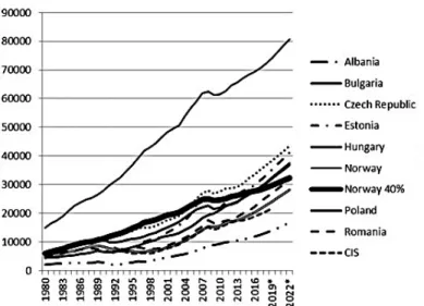
We illustrate this theoretical reasoning with some data in Figure 2. Before the collapse of centrally planned economies in 1989, the average income level in all communist countries, except Albania, was at about the 40% threshold, calculated in respect to Norway. Norway is chosen as the benchmark country in spite of the fact, that Luxemburg is the country with the highest per capita income in the region. In terms of population and terrestrial surface, Norway is more acceptable as a benchmark country. The farther away from Norway is the respective country, the less plausible is the latter hypothesis.
The 40% point is locus, where the marginal relative social utility of income is zero. An increase of average income above this level is unacceptable in the communist countries since high income has negative (in ideological terms) social utility (it tacitly implies a western way of life). Low level is also unacceptable since it indicates negative incentives, and when average income is substantially below the benchmark, workers are supposed to diminish their working efforts.
So stabilising all income levels around 40% is the needed stable solution. This corresponds to a kind of egalitarian and implicit flat income tax, securing the provisional socio-economic stability of the command economies.
The transition period of 1989–2002, however, is characterised (with some ex- ceptions) by protracted decline or stagnation of comparative real per capita in- come. All represented countries fell below the 40% level. Only after 2005, some countries returned to, or slightly improved, the command economy relative in- come pinnacle. Such deep and lingering periods of real comparative per capita
Figure 1. Marginal relative social utility of income (vertical axis) at different levels of relative income (horizontal axis)
Source: Authors’ calculations based on equation (4).
income decline are not typical for conventional boom and bust cycles and have significant socio-economic consequences. The transitional recession and the sub- sequent relative real income decline is evidently one of the reasons for propor- tional taxation propagation among the post-communist countries. However, since Figure 1 reflects purely mathematical properties and Figure 2 reflects purely em- pirical ones, we observe amazing empirical confirmation for some theoretical deductions.
This does not mean that the implementation of proportional taxation is the right answer to the economic problems of transition. The function in (3) admits any Pareto optimal redistribution. Even the best performers, such as the Czech Republic, succeeded with or without flat taxation only to reproduce or slightly improve the command economy performance in relative terms. The absolute and relative decline of average income means that the economic policy is maximum Pareto income restricting, yet not optimal. The flat tax is a sort of simple policy response to an economically hampered course of actions.
To conclude, both functions in equations (1) and (3) are fundamentally based on the existence of strong connection between diminishing marginal utility of income and the society’s aversion to inequality. The difference is that in equation (1) we assume that the coefficient of aversion to equality is positively related to real income level and is always non-negative, while in equations (3), (4) and (5)
Figure 2. GDP per capita in PPP dollars in selected countries, 1980–2022 Note: 2018–2022: Forecast.
Source: IMF Database.
the contribution of marginal social utility of income varies from positive for in- come levels below 40% to negative for high incomes. In both cases, however, the law of diminishing marginal utility of income determines the social aversion to inequality. The function in (3) has the advantage of being more compatible with the transition objectives, namely narrowing the income gap with the developed market economies.
3. METHODOLOGY
The main hypothesis of our research is that diminishing marginal utility of income is the principal reason for the flat tax adoption in the post-communist countries.
The higher the average per capita income, the stronger is the social aversion to inequality. We test a particular form of aversion to inequality, based on equations (3) and (4). In principle, Atkinson social welfare function is also compatible with the increasing aversion to inequality principle.
However, according to equations (3) and (4), the aversion to inequality and the marginal social utility of income are explicitly not constant and depend on the deviation of average income in the selected countries from the average income in the benchmark country, which must be the richest commensurate country. While Atkinson welfare function is defined in absolute money metrics, equations (3) and (5) are measurable in comparative terms with the highest income as a unit.
The social aversion to inequality in the three equations (1), (3) and (5) can be as- sumed to depend not only on income but also on risk and other factors.
We try to check our hypothesis using probit panel linear regression model.
The dependent variable takes value 0 (progressive taxation) and 1 (proportional taxation). In some cases, it is difficult to distinguish between progressive and proportional taxation, especially when the principle of horizontal progressivity is applied (Estonia) or when the differences between higher and lower taxation rates are small (Ukraine). In such cases, we keep to the official definitions.
Since we apply equation (3) as the basis of our evaluation, instead of the func- tion in equation (2), we assume the following latent variable function:
* *( , , )
i i a
y y y ρ ξ (6)
where y*i is the respective latent variable of the probit model. The difference between equations (2) and (6) is the range of the dependent variable. While e is by definition non-negative, y*i can take both positive and negative values. This makes equation (6) more compatible with equations (3) and (4) than with equa- tion (1). We also assume that the unobserved latent variable is linearly dependent on average income, risk and institutional factors:
(7)
where β0, β1, β2 and β3 are coefficients and ui is the error term. Here, we measure the average income ya as the deviation of income in the respective country from the 40% level of income in the benchmark country; the risk is measured as the average annual sovereign credit default swap (CDS) quotation, and institutional factors ξ are approximated by the binary variable taking value 1 when the respec- tive country has agreement with IMF and 0 when there is no such agreement.
The choice to use IMF relations as a proxy for institutional and policy factors is determined by the fact that the IMF supported programs are established on detailed assessment of the economic situation of the respective countries, and when proportional taxation is not compatible with macroeconomic stability, it is usually rejected.
Further, we assume the following relationship between the latent variable and the dependent binary variable is as follows:
* *
0 0; 1 0
i i i i
z if y z if y (8)
where zi is the dependent binary variable (flat or progressive income tax) and y*i is the latent variable. By applying probit regression, we explain zi in terms of ya, ρ and ξ, but we do not evaluate explicitly y*i or e.
Our comparative analysis is focused on explaining the post-communist coun- tries’ choice of personal income taxation system, so we limit the research to the geographical region of Eurasia, where mutual comparisons of income levels are possible, and labour mobility is sufficiently high.
The statistics are from the IMF data base for 42 countries1 and cover a period of 16 years from 2000 to 2015. The software package EViews 7 is used for the calculations.
1 Albania, Armenia, Austria, Belarus, Belgium, Bosnia and Herzegovina, Bulgaria, Czech Rep., Croatia, Cyprus, Finland, France, Denmark, Estonia, Germany, Georgia, Great Britain, Greece, Holland, Hungary, Iceland, Ireland, Italy, Kazakhstan, Kirgizstan, Latvia, Lithuania, Macedonia, Malta, Norway, Poland, Portugal, Romania, Russia, Serbia, Slovak Rep., Slove- nia, Spain, Sweden, Switzerland, Turkmenistan and Ukraine.
*
0 [ 1 2 3]
a
i i
y
y β ρ β β β u
ξ
4. EMPIRICAL RESULTS
We start our empirical research with Granger causality test between binary vari- able for choice of tax system, taking values 1 (flat tax) and 0 (progressive taxa- tion), and real income per capita. The results are displayed in Appendix 1. The data reveal the strong impact of GDP per capita on the choice between flat and progressive taxation and weak feedback link. In other words, the introduction of proportional taxation does not have in general measurable effect on real income.
This result is similar to other researchers’ conclusions (see for example Ivanova et al. 2005).
The main results from the probit regression are reported in Appendix 2. The regression coefficients of the explanatory variables (GDP stands for real income per capita deviation from 40% of the wealthiest country; CA is a binary variable depending on whether the respective country has an agreement with IMF at a par- ticular year, and CDS is the average annual credit default swap quotation) have the right signs and are largely significant.
In particular, the coefficient related to real income per capita and the imple- mentation of proportional taxation is negative. This result reflects the impact of diminishing marginal utility of income, that is, the lower the average income, the stronger the social resistance against progressive taxation and vice versa. The co- efficient for binary variable CA, having an agreement with the IMF, is also nega- tive. This is interpreted in the sense that agreements with IMF favour progressive taxation. The explication is that progressive taxation is, in general, fiscal income improving, so the countries with fiscal deficits, which are the usual clients of IMF, are not encouraged to introduce flat taxation.
And finally, the CDS coefficient has positive value, and thus, reflects the af- firmative relationship between risk and proportional taxation. This is also inter- preted in favour of the law of diminishing marginal utility of income in the sense that risky income is less valuable, ceteris paribus, than the sure one. It is evident that the expected value of risky income is lower than the expected value of the same nominal sure income. Consequently, the flat tax reduces the levy on high risky incomes and may be viewed as an instrument of encouraging risk-taking.
The probit regression explains 77.5% of the proportional taxation cases and 93.18% of the cases with progressive taxation. The tests for goodness of fit also provide suitable results. So the chosen framework produces fairly good explana- tion of social decisions, concerning the choice of tax system.
5. CONCLUSIONS
The main conclusion of our research is that the propagation of the proportional taxation in the post-communist countries is not simply ideology-driven, nor a ju- dicious response to the problems of transition. It is a kind of regularity, explained by the law of diminishing marginal utility of income.
This conclusion, however, leaves the question, that is, why the proportional taxation is not applied to such extent in the developing countries with even lower per capita income compared to the post-communist states, unexplained. A pos- sible answer can be that for very low relative income levels the relationship be- tween relative income and relative marginal utility of income, becomes a virtu- ally vertical line. In other words it is very difficult to apply any traditional welfare approach to the socio-economic problems of the least developed countries since any redistribution will have high social cost in terms of marginal utility of the taxed income. One likely solution is that in the poorest countries the transfers should not be so much within these countries, but between country groups – from the richest to the poorest states. The adoption of proportional taxation only makes sense for the countries earning around 30–40% of the average income in the rich- est benchmark country (see more about the differences in terms of tax reforms between middle income and poor countries in Moore – Schneider 2004), as a re- sult of the fact that at this level of average relative income the redistribution from rich to poor does not really change the relative social welfare.
The transition has two dimensions in terms of welfare. The first dimension reflects the comparative economic efficiency of the transition economies. The second dimension stands for the marginal contribution of individual incomes to the social welfare. The flat tax policy is supposed to boost the first at the expense of the second type of welfare without significant positive results. The redistribu- tion from rich to poor around the 40 per cent level is also of limited importance from the point of view of the present study. The right answer to the transition problems is only accelerated catch-up strategy in the context of appropriate mac- roeconomic and structural policy (see for example IMF 2016).
The extensive spread of proportional taxation among the post-communist countries can be broadly explained, as emphasised, by the law of diminishing marginal utility of income. However, the relationship between this law and the social aversion to inequality is not linear. In this respect, we cannot explain the flat taxation endorsement on the basis of traditional social welfare functions, like the Atkinson function, but we need a mathematical expression allowing for varia- bility in aversion to inequality, including the negative ones. Such function turned out to be the first of the Johann Bernoulli sophomore’s dream equations.
The law of diminishing marginal utility of income is subject to controversies (Tresch 2008). One of the variants is to derive this law from the risk-averse be- haviour of economic agents. Our research does not confirm this point of view. We can view risk-averse behaviour both as a consequence and as a cause of the law of diminishing marginal utility of income. Taking risk makes sense only in the context of high monetary return expectations; yet diminishing marginal utility of income implies prudent behaviour. A risk premium is necessary to keep the over- all utility of income at least constant compared to the same level of sure income.
Progressive taxation under transitional uncertainty would mean that risk pre- mium is appropriated by the state. But since the transition is necessarily associ- ated with high social and economic insecurity, the flat taxation may be viewed also as a legitimate compensation to the risk-takers. However, rewarding the risk-takers under the transitional uncertainty does not typically create a positive feedback for the rest of the population. The relative performance of virtually all transition countries worsens after the start of the market-oriented reforms. Fi- nally, the question is whether the economic policy should encourage risk-taking or try to stabilise the economy.
What is the future of the proportional taxation in the post-communist coun- tries? On the one hand, the positive results, expected from the flat tax, are in general overvalued. Most of the countries, implementing this type of taxation, are still not only lagging behind the developed market economies in terms of income per capita but are performing comparatively worse, judged against the socialist economic period. This creates a hazard for path dependence since low relative income reproduces conditions for proportional taxation. The latter, via its inabil- ity to contribute to overcome the economic inconveniencies the post-communist countries are facing, reproduces itself. On the other hand, a successful catching- up economic development creates conditions for a gradual abandonment of the flat tax practices.
REFERENCES
Atkinson, A. B. (1970): On the Measurement of Inequality. Journal of Economic Theory, 2(3):
244–263. DOI: 10.1016/0022-0531(70)90039-6.
Barbera, S. – Hammond, P. – Seidl, C. (eds) (2004): Handbook of Utility Theory. Volume 2: Exten- sions. University of East Anglia, Norwich, U.K.
Borsboom, D. – Mellenbergh, G. J. – van Heerden, J. (2003): The Theoretical Status of Latent Vari- ables. Psychological Review, 110(2): 203–219. DOI: 10.1037/0033-295x.110.2.203.
Dhillon, A. – Mertens, J. F. (1999): Relative Utilitarianism. Econometrica, 67(3): 471–498.
Easterlin, R. A. (2004): Diminishing Marginal Utility of Income? A Caveat. University of South- ern California Law School Law and Economics, Working Paper Series, No. 5. DOI: 10.1007/
s11205-004-8393-4.
European Commission (2017): The Impact of Taxes on the Competitiveness of European Tourism.
Final Report. PricewaterhouseCoopers LLP (PwC), October 2017.
Flemming, J. – Micklewright, J. (1999): Income Distribution, Economic Systems, and Transition.
Innocenti Occasional Papers Economic and Social Policy Series, No. 70. DOI: 10.1016/s1574- 0056(00)80017-2.
Fried, B. H. (1999): The Puzzling Case for Proportional Taxation. Chapman Law Review, 2(57):
157–195.
Hall, R. E. – Rabushka, A. (1995): The Flat Tax in 1995. Hoover Institution, Stanford University, January 1995, http://web.stanford.edu/~rehall/Flat%20Tax%201995.pdf
IMF (2016): Regional Economic Issues. Central, Eastern, and South Eastern Europe: How to Get Back on the Right Track. May 2016.
Ivanova, A. – Keen, M. – Klemm, A. (2005): The Russian Flat Tax Reform. IMF Working Paper, No.16. DOI: 10.5089/9781451860351.001.
Kalchev, E. (2014): The Bulgarian Flat Tax. Economic Alternatives, 1: 33–41. DOI: 10.2139/ ssrn.
2237417.
Kaneko, M. – Nakamura, K. (1979): The Nash Social Welfare Function. Econometrica, 47(2):
423–435.
Kaplow, L. (2003): Taxation and Redistribution: Some Clarifi cations. Harvard Law School, Cam- bridge, Discussion Paper, No. 424. DOI: 10.2139/ssrn.437481.
Kawano, L. – Slemrod, J. (2018): A Cross-Country Examination of Tax Systems Changes: New Evidence from a Novel Database. Presentation at the Workshop on Evaluating Tax Reforms, held at the IMF, on April 26, 2018.
Kesselman, J. R. – Irwin, G. (1978): Professor Friedman, Meet Lady Rhys-Williams: NIT vs. CIT.
Journal of Public Economics, 10(2): 179–216. DOI: 10.1016/0047-2727(78)90035-x.
Kolodko, G. W. (2000): Globalization and Catching-Up: From Recession to Growth in Transition Economies. IMF Working Paper, No. 100. DOI: 10.5089/9781451852394.001.
Mitchell, D. J. (2007): The Global Tax Revolution. Cato Policy Report, XXIX(4): 1–12. https://
object.cato.org/sites/cato.org/fi les/serials/fi les/policy-report/2007/7/cpr29n4-1.pdf
Moore, M. – Schneider, A. (2004): Taxation, Governance, and Poverty: Where Do the Middle-Income Countries Fit? Institute of Development Studies (IDS), Working Paper, No. 230, Brighton.
Novokmet, F. – Piketty, T. – Zucman, G. (2017): From Soviets to Oligarchs: Inequality and Prop- erty in Russia 1905–2016. WID.world, Working Paper Series, No. 09.
Paulus, A. – Peichl, A. (2008): Effects of Flat Tax Reforms in Western Europe on Income Distribu- tion and Work Incentives. IZA DP, No. 3721. DOI: org/10.2139/ssrn.1106173.
Polemarchakis, H. M. – Siconolfi , P. (1993): Competitive Equilibria without Free Disposal or Non- satiation. Journal of Mathematical Economics, 22: 85–99.
Pomerleau, K. – Hodge, S. – Walczak, J. (2017): International Tax Competitiveness Index 2017.
Washington, D. C.: Tax Foundation.
Rawls, J. (1971): A Theory of Justice. Harvard University Press.
Saavedra, P. (2007): Flat Income Tax Reforms. In: Gray, Ch. – Lane, T. – Varoudakis, A. (eds): Fis- cal Policy and Economic Growth: Lessons from Eastern Europe and Central Asia. The World Bank, Washington, D.C.
Takayama, A. (1990): Mathematical Economics. Cambridge University Press.
Tresch, R. W. (2008): Public Sector Economics. Palgrave/Macmillan.
Vecernik, J. (1999): Communist and Transitory Income Distribution and Social Structure in the Czech Republic. UNU, World Institute for Development Economics Research (UNU/WIDER).
DOI: 10.2139/ssrn.323201.
Young, H. P. (1987): Progressive Taxation and the Equal Sacrifi ce Principle. Journal of Public Economics, 32(2): 203–214. DOI: 10.1016/0047-2727(87)90012-0.
APPENDIX 1
Granger Causality Tests between binary variable (Prob) and income per capita (GDP) with lags of 2, 4 and 6 years
Pairwise Granger Causality Tests Sample: 2000–2015
Lags: 2
Null hypothesis: Obs F-Statistic Prob.
PROB does not Granger Cause GDP 602 1.33597 0.2637
GDP does not Granger Cause PROB 14.8463 5.E-07
Lags: 4
Null Hypothesis: Obs F-Statistic Prob.
PROB does not Granger Cause GDP 516 0.30700 0.8733
GDP does not Granger Cause PROB 8.84038 7.E-07
Lags: 6
Null hypothesis: Obs F-Statistic Prob.
PROB does not Granger Cause GDP 430 0.33963 0.9157
GDP does not Granger Cause PROB 5.28578 3.E-05
APPENDIX 2
Dependent variable: PROB
Method: ML - Binary Probit (Quadratic hill climbing) Sample (adjusted): 2007–2015
Included observations: 256 after adjustments Convergence achieved after 5 iterations
Covariance matrix computed using second derivatives
Variable Coefficient Std. Error z-Statistic Prob.
C –0.273056 0.241507 –1.130632 0.2582
GDP –0.091704 0.012847 –7.138206 0.0000
IMF program –0.745313 0.264803 –2.814599 0.0049
Credit Default Swap 0.101630 0.078533 1.294107 0.1956 McFadden R-squared 0.478846 Mean dependent var 0.312500 S.D. dependent var 0.464420 S.E. of regression 0.305926 Akaike info criterion 0.678614 Sum squared resid 23.58486 Schwarz criterion 0.734007 Log likelihood –82.86257
Hannan-Quinn criter. 0.700893 Deviance 165.7251
Restr. deviance 317.9962 Restr. log likelihood –158.9981 LR statistic 152.2711 Avg. log likelihood –0.323682 Prob(LR statistic) 0.000000
Obs with Dep=0 176 Total obs 256
Obs with Dep=1 80
Categorical Descriptive Statistics for Explanatory Variables
Mean
Variable Dep=0 Dep=1 All
C 1.000000 1.000000 1.000000
GDP 16.46291 –7.951328 8.833462
IMF program 0.187500 0.275000 0.214844
Credit Default Swap 1.580114 3.327500 2.126172
Standard Deviation
Variable Dep=0 Dep=1 All
C 0.000000 0.000000 0.000000
GDP 15.30538 11.28888 18.13298
IMF program 0.391426 0.449331 0.411518
Credit Default Swap 1.264912 1.755568 1.646642
Observations 176 80 256
Expectation-Prediction Evaluation for Binary Specification Success cutoff: C = 0.5
Estimated Equation Constant Probability
Dep=0 Dep=1 Total Dep=0 Dep=1 Total
P(Dep=1)<=C 164 18 182 176 80 256
P(Dep=1)>C 12 62 74 0 0 0
Total 176 80 256 176 80 256
Correct 164 62 226 176 0 176
% Correct 93.18 77.50 88.28 100.00 0.00 68.75
% Incorrect 6.82 22.50 11.72 0.00 100.00 31.25
Total Gain* –6.82 77.50 19.53
Percent Gain** NA 77.50 62.50
Estimated Equation Constant Probability
Dep=0 Dep=1 Total Dep=0 Dep=1 Total
E(# of Dep=0) 149.57 25.71 175.28 121.00 55.00 176.00
E(# of Dep=1) 26.43 54.29 80.72 55.00 25.00 80.00
Total 176.00 80.00 256.00 176.00 80.00 256.00
Correct 149.57 54.29 203.86 121.00 25.00 146.00
% Correct 84.98 67.86 79.63 68.75 31.25 57.03
% Incorrect 15.02 32.14 20.37 31.25 68.75 42.97
Total Gain* 16.23 36.61 22.60
Percent Gain** 51.94 53.25 52.60
* Change in “% Correct” from default (constant probability) specification.
** Per cent of incorrect (default) prediction corrected by equation.
Goodness-of-Fit Evaluation for Binary Specification Andrews and Hosmer-Lemeshow Tests
Grouping based upon predicted risk (randomize ties)
Quantile of Risk Dep=0 Dep=1 Total H-L
Low High Actual Expect Actual Expect Obs Value
1 4.E-09 0.0017 24 24.9913 1 0.00873 25 112.583
2 0.0018 0.0040 25 25.9255 1 0.07447 26 11.5348
3 0.0041 0.0157 25 24.7479 0 0.25210 25 0.25467
4 0.0161 0.1038 26 24.9256 0 1.07437 26 1.12068
5 0.1051 0.2152 26 21.8609 0 4.13907 26 4.92275
6 0.2169 0.3204 25 18.3153 0 6.68467 25 9.12441
7 0.3295 0.4892 11 15.4096 15 10.5904 26 3.09787
8 0.4893 0.6783 5 10.4878 20 14.5122 25 4.94670
9 0.6816 0.8247 7 6.49710 19 19.5029 26 0.05189
10 0.8287 0.9961 2 2.11665 24 23.8833 26 0.00700
Total 176 175.278 80 80.7223 256 147.644
H-L Statistic 147.6441 Prob. Chi-Sq(8) 0.0000 Andrews Statistic 108.1494 Prob. Chi-Sq(10) 0.0000