Assessing the accuracy of three classical DFTs of the electrical double layer
Adelina Voukadinova1,2, Mónika Valiskó3, and Dirk Gillespie2,*
1University of Illinois at Chicago, Chicago, IL, USA
2Department of Physiology and Biophysics, Rush University Medical Center, Chicago, IL, USA
3Department of Physical Chemistry, University of Pannonia, Veszprém, Hungary
*corresponding author: dirk_gillespie@rush.edu
16 April 2018
ABSTRACT
Classical Density Functional Theory (DFT) is a useful tool to compute the structure of the electrical double layer because it includes ion-ion correlations due to excluded-volume effects (i.e., steric correlations) and ion screening effects (i.e., electrostatic correlations beyond the electrostatic mean-field potential). This paper systematically analyzes the accuracies of three different electrostatic excess free energy functionals, as compared to Monte Carlo (MC) simulations of the planar electrical double layer, over a large parameter space. Specifically, we tested the reference fluid density (RFD) (J. Phys.: Condens. Matter 14, 12129), functionalized mean spherical approximation (fMSA) (J. Phys.: Condens. Matter 28, 244006), and bulk fluid (BF) (Phys. Rev. A 44, 5025; J. Chem. Phys. 98, 8126) functionals. Previous work compared these DFT methods to MC simulations only for a small set of parameters. Here, a total of twelve different cations were studied, with valences of +1, +2, and +3 and ion diameters of 0.15, 0.30, 0.60, and 0.90 nm at bulk concentrations between 1 μM and 1 M. The anion always had valence –1 and diameter 0.30 nm. The structure of the double layer of these charged, hard-sphere ions was computed for surface charges ranging from 0 to –0.50 C/m2. All the DFTs were compared against each other for all the parameters, as well as to 378 MC simulations. Overall, RFD was the best of the three functionals, while BF was the least accurate. fMSA performed significantly better than BF, making it a reasonable choice that is less computationally expensive than RFD.
For monovalent cations, all three functionals worked reasonably well, except BF was qualitatively different from MC at very low surface charges. For multivalent cations, BF underestimated charge inversion while fMSA overestimated it. All DFTs performed poorly for small multivalent ions.
INTRODUCTION
Even though the electrical double layer has been studied for well over a century, it has regained importance in far-ranging modern technologies, including energy (e.g., electrochemical supercapacitors [1] and energy conversion [2, 3]) and analytical chemistry (e.g., nanopore DNA sequencing [4, 5] and analyte detection [6-9]). Some of these applications utilize the capacitance of the electrical double layer to store charge, while others exploit atomic scale ion-ion correlations to produce macroscopic effects. For instance, the finite size of ions near a highly
charged electrode can produce long-range density oscillations that can, in principle, be used to increase the efficiency of pressure-to-voltage energy conversion [10]. In addition to these steric correlations, electrostatic correlations that produce charge inversion can be exploited to produce a stable front between two electrolytes [11] or change the direction of a column of fluid [12].
In order to understand the physics of these systems and to optimize existing (and design new) capabilities, accurate modeling of the electrical double layer is more important than ever.
All-atom molecular dynamics simulations would be ideal, but they are computationally intensive. Moreover, they cannot simulate the low concentrations and applied voltages of real- world applications and of experiments. On the other hand, reduced models, which approximate some of the physics and simplify the representation of the atoms and molecules involved, can.
They have reproduced experiments in a variety of fields, including biology [13] and nanofluidics [14, 15], because their approximations still capture the overall physics driving the device [16].
One of the oldest and most widely used reduced models of electrolytes is the primitive model of ions in which the ions are charged, hard spheres and water is a background dielectric [17]. Near a charged surface, this simple model produces both steric correlations (i.e., oscillatory density profiles) and electrostatic correlations (i.e., the surplus of co-ions behind the initial layer of counterions that is characteristic of charge inversion and that may change the sign of the electrostatic potential) [18, 19]. For this system, Monte Carlo (MC) simulations have the most accurate results for the density and electrostatic potential profiles of the double layer.
Another technique to calculate the structure of the electrical double layer with charged, hard-sphere ions is classical density functional theory (DFT). In DFT, a mathematical relationship between the free energy of the system and the ion density profiles is constructed and then minimized to find the equilibrium profiles. This necessarily involves approximations, as the exact relationship between the free energy and the density profiles is not known. Various approximations have yielded a number of different DFTs of charged hard-sphere fluids. Here, we focus on three of these: the bulk-fluid (BF) DFT [20, 21], the reference fluid density (RFD) DFT [22, 23], and the functionalized mean spherical approximation (fMSA) DFT [24]. BF is one of the earliest and most commonly used DFTs of charged systems, while fMSA is one of the newest. RFD is more computationally involved, but has the advantage of being applicable to two-phase systems, while the other two are not. For all three of these DFTs, accurate density and potential profiles (as compared to MC simulations) have been reported [20-25]. Because of this
accuracy and because DFT calculations are substantially faster than MC simulations (at least in simple geometries), DFT has established itself as an important theory for computing the structure of the electrical double layer.
What has been missing, however, is a systematic analysis of where DFT is accurate and where it is not. This is what we attempt to do here by comparing the BF, RFD, and fMSA DFTs to a new set of MC simulation results that spans a wide range of conditions (specifically, low to high ion concentrations, mono- and multivalent ions, small to large ion size, and low to high electrode surface charges) [26]. So far, DFTs have been compared to only a scattershot of MC simulations, and a more systematic evaluation is necessary for several reasons. First, defining the limits of applicability of any theory (and these three DFTs in particular) will allow us to apply it with confidence in future applications. Here, we find that each of the three DFTs we test have very different limits of applicability. Second, knowing that a DFT works over a large range of parameters will open up new uses for it. For example, trends in double layer properties can be computed to better understand the physics of ion-ion correlations (e.g., varying the surface charge to better understand the onset of charge inversion). Lastly, a systematic analysis will point to areas where DFT in general will need to be improved. We find, for example, that trivalent ions (especially very small ones) are not well-modeled by any of the three DFTs tested here.
THEORY AND METHODS Three Functionals
DFT is defined by the principal that there exists a free-energy functional [{ ( )}]Ω ρi x of arbitrary density profiles ( )ρi x in three-dimensional space such that those density profiles that minimize the functional are the equilibrium density profiles [27]. Once an approximate free- energy functional is constructed, the functional can be minimized directly or by solving the Euler-Lagrange equations that result from the variational principle δΩ/δρi( ) 0x = for all ion species i. In practice, the Ω is divided into an ideal gas and excess components:
id ex
[{ ( )}]ρi F [{ ( )}]ρi F [{ ( )}]ρi
Ω x = x + x . Since the ideal gas component is known exactly,
deriving approximate free-energy functionals focuses on the excess component Fex[{ ( )}]ρi x .
For Coulombic systems of charged, hard spheres, this term is generally divided into hard- sphere (superscripted HS) and electrostatic components (superscripted ES), and the electrostatic component is further divided into the mean-field term (superscripted MF), which produces the mean electrostatic potential φ( )x calculated from the density profiles via the Poisson equation, and the remainder term that we call the screening term (superscripted SC):
ex HS ES
HS MF SC
[{ ( )}] [{ ( )}] [{ ( )}]
[{ ( )}] [{ ( )}] [{ ( )}].
i i i
i i i
F F F
F F F
ρ ρ ρ
ρ ρ ρ
= +
= + +
x x x
x x x (1)
The hard-sphere component is relatively well-established and accurate through Rosenfeld’s fundamental measure theory approach (reviewed by Roth [28]). For all the calculations shown here, we use the White Bear Mark I functional [29].
Next, we briefly describe the three screening functionals we analyze, but the reader is referred to the original papers for complete details.
The BF functional expands FSC around a reference density profile with known properties using a second-order functional Taylor expansion. In practice, this is usually the bulk fluid with which the system is in equilibrium [20, 21] and the necessary first- and second-order direct correlation functions taken from the mean spherical approximation (MSA) [30-32].
The RFD functional [22, 23] starts with the same Taylor expansion idea, but constructs a reference density profile “on the fly” using the current guesses for the density profiles ( )ρi x . First, new density profiles ρi*( )x are made from the current density profiles by making those profiles be charge neutral and have the same ionic strength as the ( )ρi x at every grid point x.
These ρi*( )x are then averaged over a sphere whose radius is the screening length at x to produce density profiles ( )ρi x . This local screening length is determined by having the MSA screening length, applied pointwise, of ( )ρi x be the same screening length used to average the
*( )
ρi x . In this way, the local screening length is self-consistently determined. Because the screening length is relatively long, the reference profiles ( )ρi x are smooth and slowly varying in space and, by construction, charge neutral so that all MSA formulas for the first- and second- order correlation functions can be applied pointwise. This approach has the advantage that the reference fluid densities change with the density profiles ( )ρi x and therefore can adjust to interface phenomena like gas-liquid equilibrium and semi-permeable membranes. This is not so
in the BF approach, where the bulk fluid density on one side of the interface must be used, and different choices give different answers [23]. The cost of this wider range of applicability is the additional cost of computing the local screening length at every grid point at every iteration of the solution algorithm. In addition, this produces different size spheres to average over to make the ( )ρi x , something that cannot be calculated directly with the standard fast Fourier methods used throughout DFT.
The fMSA functional was designed to mitigate this computational cost while still retaining a high level of accuracy. The basic foundation of the fMSA approach is based on an observation by Blum and Rosenfeld [33] that both the first- and second-order direct correlation functions of the MSA can be written in terms of spherical shells of charge at the capacitance radius of the ions (i.e., the ion radius plus the MSA screening length). By averaging the density profiles over this capacitance radius and using them in the MSA formula for the free energy density, the fMSA functional was derived. Because the capacitance radius was chosen to be that of the bulk fluid, all averaging was done with a single sphere size that allows the use of fast Fourier transform methods.
Assessing Double Layer Structure
Density profiles of cations ( ( )ρ+ x ) and anions ( ( )ρ− x ) were calculated near a hard, smooth wall with surface charge σ located at x = 0, assuming homogeneity in the y-z plane parallel to the wall. We minimized the RFD, fMSA, and BF functionals by directly solving the Euler-Lagrange equations using the fixed-point methods described previously [28, 34] over a finely-spaced grid that ensured at least 60 points per ion diameter. We compared these results to MC simulations by Valiskó et al. [26]. The parameter spaces explored with the DFT calculations and MC simulation are shown in Table 1.
To compare RFD and fMSA, we wanted to quantify profile similarity. We first calculated the root mean square of the difference (RMSD) to emphasize any large gaps between the profile sets. Specifically, we determined the RMSD between RFD and fMSA profiles for ( )ρ+ x , ( )ρ− x , and φ( )x for all grid points up to 3d+ and starting at the contact values x d= + / 2, / 2,d− and 0, respectively. This was done because we wanted to focus on where the profiles changed the most with x and therefore might be the most different.
We also calculated the Pearson correlation coefficient for the RFD and fMSA ( )ρ+ x , ( )x
ρ− , and φ( )x . This was done to compare profile shapes. Specifically, the correlation coefficient assesses whether two profiles are increasing or decreasing over the grid points we studied (the same x intervals as the RMSD calculations). Therefore, a correlation coefficient that is far from 1 indicates less qualitative agreement, even if the RMSD between the curves is small.
Combining these two methods highlights both differences in scale (RMSD) and qualitative shape (correlation coefficient) so that we could assess where RFD and fMSA profiles were different. Areas of difference then indicate that the two diverge and it is especially important to compare these regions to MC simulations to assess which DFT is more accurate.
Where they were the same, we also compared them to MC results and found equally good accuracy. While we will focus mainly on discussing the differences, the figures will also show the similarities.
Capacitance
The final comparison is done only for the electrostatic potential profiles, specifically the difference in surface potentials (electrostatic potentials) for RFD and fMSA at the charged surface: ∆ =φ φRFD(0)−φfMSA(0). This comparison is useful for understanding the accuracy of the capacitance. Areas with large ∆φ values indicate an inconsistency between the two DFT
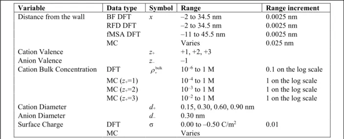
Variable Data type Symbol Range Range increment
Distance from the wall BF DFT x –2 to 34.5 nm 0.0025 nm
RFD DFT –2 to 34.5 nm 0.0025 nm
fMSA DFT –11 to 45.5 nm 0.0025 nm
MC Varies 0.025 nm
Cation Valence z+ +1, +2, +3
Anion Valence z– –1
Cation Bulk Concentration DFT ρ+bulk 10–6 to 1 M 0.1 on the log scale MC (z+=1) 10–4 to 1 M 1 on the log scale MC (z+=2) 10–3 to 1 M 1 on the log scale MC (z+=3) 10–2 to 1 M 1 on the log scale
Cation Diameter d+ 0.15, 0.30, 0.60, 0.90 nm
Anion Diameter d– 0.30 nm
Surface Charge DFT σ 0.00 to –0.50 C/m2 0.01
MC Varies
Table 1. Parameters varied in the DFT calculations and the MC simulations. In the DFT calculations, the same surface charges and concentrations (3111 combinations) were computed for all 12 cations.
profiles, and are then looked at more in depth by plotting ∆φ versus σ for every ρ+bulk to determine whether RFD or fMSA is more accurate.
BF Functional
We also did this large-scale comparison for BF versus RFD (since we generally found it to be more accurate). While of interest, these and some other results pertaining to the BF function are shown in the Appendix. In the main text, we show the BF profiles along with the other RFD, fMSA, and MC results, and our assessment of the BF functional follows from these comparisons.
RESULTS AND DISCUSSION Double Layer Structure
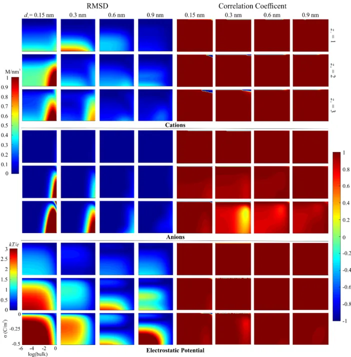
The plots for the RMSD and Pearson coefficient comparisons for RFD versus fMSA are shown in Figure 1. (The corresponding comparisons for RFD versus BF are show in the Appendix in Fig. A1.) For the cation and anion density profiles, overall, there is a similarity between RFD and fMSA with a few scattered pockets of differences. For φ( )x there are more significant differences that will be further explored in the capacitance subsection. In general, all three profiles are quantitatively and qualitatively very similar when the ions have a 0.30 nm diameter (all ions have the same size) and for monovalent ions.
Six discrete groups are visible in Figure 1 that display differences between the two functionals. After a brief description, each will be discussed in turn. Groups 1 and 2 both focus on the high inverse correlation coefficients: Group 1 is at low ρ+bulk and σ = 0 C/m2 and Group 2 at d+ = 0.15 nm with z+ = 2 and 3. Group 3 is the RMSD variation at d+ = 0.15 nm with z+ = 2 and 3 at high σ where all three profiles show deviation. Group 4 is the RMSD variation at d+ = 0.60 and 0.90 nm with z+ = 2 and 3 for ( )ρ− x and φ( )x , although from the RMSD plots it is not as apparent that there is ( )ρ− x variation at low ρ+bulk. Group 5, which has the least variation out of all the groups, focuses on ions with d+ = 0.30 nm at high σ, specifically at z+ = 1 and 3 for
( )x
ρ+ and ρ−( )x respectively. Lastly, Group 6 focuses on the weak correlation in the anion profiles for trivalent ions.
For the first group at z+ = 1 and 2 across all diameters, an inconsistency in Figure 1 is present at low ρ+bulk and σ = 0 C/m2 for both ( )ρ+ x and ρ−( )x correlation coefficient plots.
These sections of the plots have correlation coefficients near –1. However, these are artifacts due Fig. 1. Plots comparing the RMSD (left) and the Pearson correlation coefficients (right) for RFD and fMSA ( )ρ+ x (top), ( )ρ− x (middle), and φ( )x (bottom). The logarithm of ρ+bulk is shown on the x-axis and σ is shown on the y-axis of each individual plot. Each row of plots corresponds to z+ and the columns to d+ as indicated. The group numbers of areas of difference are shown near the corresponding areas with significant deviation. The maximum values for the RMSD scales are 2.46 M (cations and anions) and 5.67 kT/e (electrostatic potential); this results in oversaturation for some of the plots.
to the functionals having a small difference in contact value (data not shown). RFD has a contact density just above ρ+bulk and fMSA just below. This causes the profiles for RFD to monotonically decrease to ρ+bulk and fMSA to increase to ρ+bulk making them quantitatively the same, but with an anticorrelated slope. This occurs for σ = 0 only.
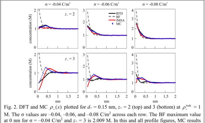
For the second group, we analyze some representative cases of negative correlation coefficients seen in Figure 1 at d+ = 0.15 nm and z+ = 2 and 3. Figure 2 shows the cation profiles plotted at σ = –0.04, –0.06, and –0.08 C/m2 and ρ+bulk = 1 M. At z+ = 2 with σ = –0.04 C/m2, fMSA has qualitative differences by peaking twice at a smaller height in the same domain that RFD and MC peak once. At z+ = 3, fMSA and MC have quantitatively similar peak height magnitudes, but have differences in curve shape and contact density (at x = d+/2). RFD deviates significantly from both by having an absolute minimum in the domain where fMSA and MC have an absolute maximum for σ = –0.06 and –0.08 C/m2. Overall, RFD and MC are similar at z+
= 2, and fMSA and MC are similar at z+ = 3. Lastly, the BF functional produces a substantially larger contact density and a curve that does not resemble the fMSA, RFD, or MC curves.
Fig. 2. DFT and MC ( )ρ+ x plotted for d+ = 0.15 nm, z+ = 2 (top) and 3 (bottom) at ρ+bulk = 1 M. The σ values are –0.04, –0.06, and –0.08 C/m2 across each row. The BF maximum value at 0 nm for σ = –0.04 C/m2 and z+ = 3 is 2.009 M. In this and all profile figures, MC results are the blue symbols, RFD the solid black line, fMSA the solid red line, and BF the dashed gray line.
For the third group, we analyze the RMSD variation that is consistent across all three profiles at d+ = 0.15 nm with z+ = 2 and 3. Figure 3 shows the profiles plotted for all valences at σ = –0.50 C/m2 with ρ+bulk = 0.1 and 1 M. The monovalent ions across the three profiles show no significant variation. At z+ = 2 for both ρ+bulk, there is ( )ρ+ x variation on the log scale with fMSA and BF deviating from the overlapping RFD and MC curves. At z+ = 2 with ρ+bulk = 0.1 M for ρ−( )x , RFD peaks highest of all four curves and decreases at a faster rate than fMSA, resulting in a small curve shape discrepancy. In contrast, the BF ( )ρ− x does not peak at all.
All three profiles show significant variation for z+ = 3. For ( )ρ+ x , the RFD curves have a peak above ρ+bulk immediately after the exponential decrease for both ρ+bulk where MC and fMSA do not; the log scale shows the qualitative differences between both DFTs and MC. For ( )ρ− x at ρ+bulk = 0.1 M, RFD and fMSA are similar, but MC deviates significantly from both. At ρ+bulk = 1 Fig. 3. DFT and MC ( )ρ+ x , ( )ρ− x , and φ( )x (labeled at right) plotted for d+ = 0.15 nm and z+ = 1, 2, and 3 at ρ+bulk = 0.1 and 1 M and σ = –0.50 C/m2. The second row of plots use the log scale for the cation concentration profile.
M, fMSA and MC have a deeper minimum and decreases faster than RFD. For φ( )x at ρ+bulk = 0.1 M, a small separation occurs between the curves as they decrease. At ρ+bulk = 1 M, the DFT curves peak at different heights and RFD decreases at a dissimilar rate from MC and fMSA. The BF curve tends to fall below the other three when the ions are not monovalent, and BF exhibits little to no charge inversion for multivalent ions.
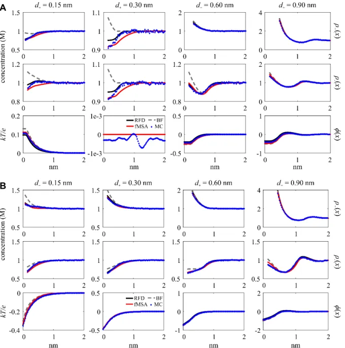
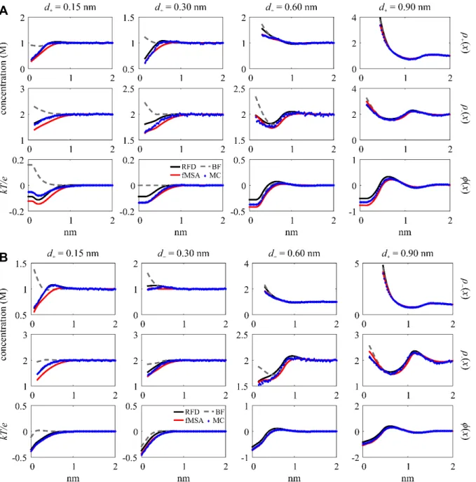
The fourth group includes the variations that are most significant for ( )ρ− x and φ( )x at large diameters. Figure 4 shows all three profiles plotted for d+ = 0.60 and 0.90 nm with z+ = 2 and 3, σ = –0.50 C/m2, and ρ+bulk = 0.01 M. Under these conditions, fMSA shows the greatest deviation from both RFD and MC while the BF curve tends to fall between RFD and fMSA. The
( )x
ρ− variation is largest at d+ = 0.60 nm, with some fMSA anion profiles having a peak about tenfold higher than RFD and MC. This can also be seen for d+ = 0.90 nm and z+ = 3. This creates Fig. 4. DFT and MC ( )ρ+ x , ( )ρ− x , and φ( )x (labeled at right) plotted for d+ = 0.60 and 0.90 nm with z+ = 2 and 3 at ρ+bulk = 0.01 and σ = –0.50 C/m2. The second row of plots use the log scale. The ( )ρ− x plot for z+ = 2 and d+ = 0.90 nm converges at x > 2.5 nm.
a change of sign in φ( )x (i.e., charge inversion) that does not exist for RFD and MC. For ( )ρ+ x on the log scale one may notice that fMSA tends to deviate from the other curves at d+ = 0.60 nm, and MC is offset from the DFTs at d+ = 0.90 nm and z+ = 2.
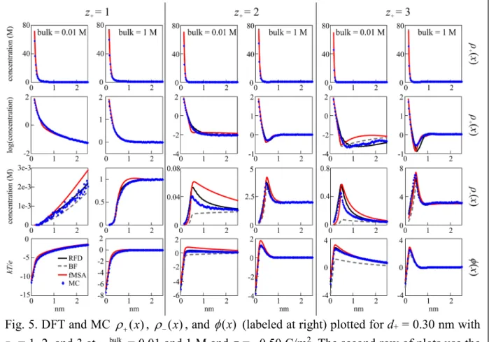
The fifth group is concerned with the small discrepancies for d+ = 0.30 nm. Figure 5 shows all three profiles plotted for d+ = 0.30 nm at all valences with σ = –0.50 C/m2 and ρ+bulk = 0.01 and 1 M. For ( )ρ+ x at z+ = 3 with ρ+bulk = 0.01 M, there is a small gap between fMSA and both RFD and MC that appears on the log scale graph. For ( )ρ− x at z+ = 2 with ρ+bulk = 0.01 M, there is a peak height difference between RFD and fMSA and an even bigger difference between fMSA and MC. The curves show qualitative differences, with fMSA decreasing roughly at a linear rate and RFD and MC at an exponential rate. The φ( )x curves show minimal disparities aside from a small quantitative difference. BF overlaps with most of the curves, but occasionally falls below the rest, again failing to predict charge inversion.
Fig. 5. DFT and MC ( )ρ+ x , ( )ρ− x , and φ( )x (labeled at right) plotted for d+ = 0.30 nm with z+ = 1, 2, and 3 at ρ+bulk = 0.01 and 1 M and σ = –0.50 C/m2. The second row of plots use the log scale. The ( )ρ− x plot for z+ = 1 and ρ = 0.01 M converges at x > 2.5 nm.
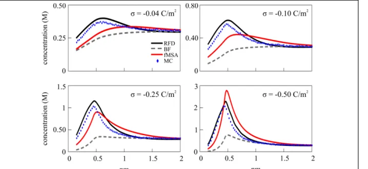
The focus of the sixth and final group is the low ( )ρ− x correlation values at d+ = 0.30 nm with z+ = 3. As shown in Fig. 6, the problem is similar to that in Group 5. Here, the fMSA peak is shifted relative to the RFD and MC peaks to a larger x. Also, both the RFD and fMSA curves increase at a similar rate, but the fMSA profile decreases at a smaller rate after the peak. In general, RFD and MC always agree. As in the previous cases shown, the BF functional fails to produce this anion peak at all.
Lastly, we describe a specific shortcoming of the BF functional. In a previous study [25]
it was noted that the BF functional was qualitatively different from MC simulations (and the Fig. 7. Plots comparing ∆φ for RFD and fMSA at the charged surface. The plot axes and arrangements are as in Figure 1.
Fig. 6. DFT and MC cation profiles ( )ρ+ x plotted for d+ = 0.30 nm with z+ = 3 at ρ+bulk = 0.1 M and σ = –0.04, –0.10, –0.25, and –0.50 C/m2.
RFD functional) at very low surface charges (including 0) and high bulk concentrations for all cation valences from +1 to +3. Here, we study this issue a little further. In the Appendix, Figs.
A2–A4 show profiles for the MC simulations and all three functionals under such conditions. In general, the BF cation and anion profiles deviate qualitatively from MC for all four cation sizes and all three valences, while the other two functionals have the correct form; the BF potential profiles are generally more accurate. However, for | | ~ 0.03σ > C/m2 the profiles match MC simulations, especially for the monovalents.
Capacitance
The surface potential results demonstrate a similar pattern as the double layer structure, with the least variation occuring for ions with d+ = 0.30 nm and for the monovalents. Figure 7 shows the plots for Δϕ at the charged surface for RFD versus fMSA. (The corresponding comparisons for RFD versus BF are shown in the Appendix in Fig. A5.) Positive ∆φ values indicate that φRFD(0)>φfMSA(0). Generally speaking, ions with d+ = 0.15 and 0.30 nm have ∆φ >
0 and ions with d+ = 0.60 and 0.90 nm have ∆φ < 0. The greatest variation occurs for z+ = 3 across all diameters, with the largest devation at d+ = 0.90 nm.
For each valence across all four diameters, we plotted ∆φ vs. σ for all available MC ρ+bulk. Figure 8 shows the plots for z+ = 1 for all four diameters and all three functionals. Overall, both curves are very close to MC. RFD more closely resembles MC, although the differences Fig. 8. Surface potential φ(0) versus surface charge σ for z+ = 1 with each set of curves representing one of the log(ρ+bulk) (0 to –4 from top to bottom).
between fMSA and RFD are minimal. For all diameters with |σ| ≤ 0.10 C/m2, both RFD and fMSA overlap MC. Overall, RFD is preferable to fMSA for |σ| ≥ 0.25 C/m2. Overall, BF is just as accurate as the other functionals for all monovalent ions.
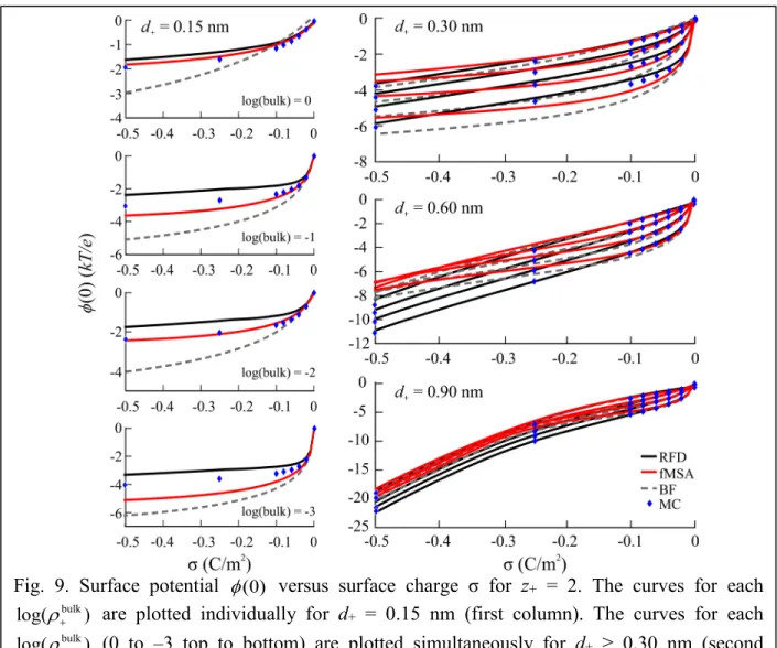
Figure 9 shows the φ(0) vs. σ plots for z+ = 2 for all four diameters. Each ρ+bulk was individually plotted for d+ = 0.15 nm. In this case, fMSA is more accurate than both RFD and BF when compared to MC. For larger divalent ions, BF closely resembles fMSA, but RFD is the most accurate DFT at high σ, while all three DFTs are reliable at low σ.
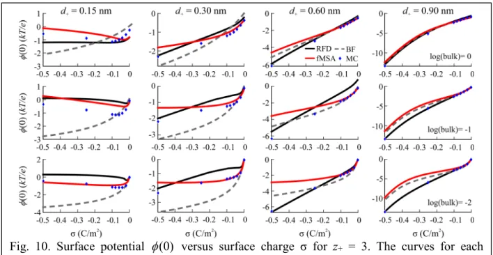
Figure 10 shows the φ(0) vs. σ plots for z+ = 3 for all four diameters with individual plots for each ρ+bulk. For d+ = 0.15, all DFT methods are completely offset from MC, although fMSA is qualitatively more accurate especially at low σ. It should be noted, however, that quantitatively Fig. 9. Surface potential φ(0) versus surface charge σ for z+ = 2. The curves for each
log(ρ+bulk) are plotted individually for d+ = 0.15 nm (first column). The curves for each log(ρ+bulk) (0 to –3 top to bottom) are plotted simultaneously for d+ ≥ 0.30 nm (second column).
they are only off by fractions of kT/e because the surface potential is so small. For d+ ≥ 0.30 nm, the preference for RFD becomes greater at high σ. For d+ = 0.30 nm, RFD is only preferable at high σ and fMSA closely resembles MC at low σ. At d+ = 0.60 and 0.90 nm, RFD is better at high σ, and all three functionals overlap MC at low σ.
CONCLUSION
All three DFT methods we tested (RFD, fMSA, and BF) have areas where they give similar results, but some functionals deviate significantly more from MC than others. Out of all three, when compared to MC simulations, RFD is the most accurate across nearly all profiles and parameters. Although not as accurate as RFD, fMSA is generally a good choice, but it tends to overestimate charge inversion and its “bump” of anions after the initial layer of cations. BF is the worst of the three as it has the largest profile deviation from MC out of all three methods. Also, BF tends to significantly underestimate charge inversion, many times exhibiting only a tiny anion bump (or none at all) when MC simulations show a significant excess over bulk. BF also is qualitatively incorrect at high bulk concentrations (above ~0.3 M) with very low surface charges, including at σ = 0, for all the ions we studied.
When looking at the structure of the double layer, all three methods work well for monovalent ions, except for BF’s problems at low surface charges. For divalent and trivalent
Fig. 10. Surface potential φ(0) versus surface charge σ for z+ = 3. The curves for each log(ρ+bulk) (0 to –2 top to bottom) are plotted individually for all d+ across each column.
ions with a 0.60 and 0.90 nm diameter, RFD is by far the most accurate DFT; fMSA and BF do not do nearly as well predicting charge inversion. None of the DFTs prove reliable for trivalent ions with a 0.15 nm diameter when comparing the double layer structure. The fMSA functional does reasonably well in this one particular case, but as ion size increases, its accuracy drops off significantly and therefore is not the best choice for trivalents overall.
When looking at the surface potential versus surface charge relationship (and therefore capacitance), all three methods are equally good for monovalent ions. For multivalent ions, fMSA is generally better for the smallest ions and works equally as well as RFD at low surface charges. Otherwise, RFD is generally more accurate. BF results are generally comparable to fMSA results.
Overall, this work shows that multivalent ions, especially small ones, are an area that can be improved in future electrostatics functionals. Especially for trivalent ions, none of the functionals we tested gave consistently good results across all ion diameters. For example, fMSA did significantly better than RFD for small trivalent ions, but lost accuracy as ion size increased; for RFD this was reversed. BF, on the other hand, always fared poorly for multivalent ions.
Lastly, this work shows the importance of the screening term in determining the structure of the electrical double layer, especially for charge inversion; each of the three functionals we tested showed varying degrees of accuracy for charge inversion. Since the RFD functional generally did best, this may indicate that using local screening lengths instead of a single one, as is done for the BF and fMSA functionals, is an avenue for improving electrostatic functionals.
ACKNOWLEDGMENTS
This material is based on work supported by the National Science Foundation under Grant 1402897 (to D.G.). The financial support of the National Research, Development and Innovation Office (NKFIH K124353) is gratefully acknowledged. Supported by the UNKP-17-4 (to M.V.), the New National Excellence Program of the Ministry of Human Capacities.
APPENDIX
This appendix contains Figs. A1–A5 that focus on BF results secondary to the main text figures.
Fig. A1. Plots comparing the RMSD (left) and the Pearson correlation coefficients (right) for the RFD and BF functionals: ( )ρ+ x (top), ρ−( )x (middle), and φ( )x (bottom). The logarithm of ρ+bulk is shown on the x-axis and σ is shown on the y-axis of each individual plot. Each row of plots corresponds to z+ and the columns to d+ as indicated. The group numbers of areas of difference are shown near the corresponding areas with significant deviation. The maximum values for the RMSD scales are 4.17 M (cations and anions) and 5.17 kT/e (electrostatic potential); this results in oversaturation for some of the plots. The same scales as in Fig. 1 of the main text are used.
A
B
Fig. A2. DFT and MC ρ+( )x , ( )ρ− x , and φ( )x (labeled at right) plotted for ρ+bulk = 1 M and σ = 0 C/m2 (A) and –0.02 C/m2 (B) for all monovalent ions across all diameters (labeled at top).
A
B
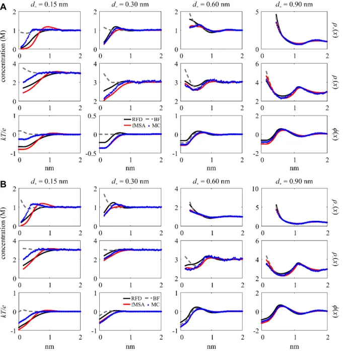
Fig. A3. DFT and MC ρ+( )x , ( )ρ− x , and φ( )x (labeled at right) plotted for ρ+bulk = 1 M and σ = 0 C/m2 (A) and –0.02 C/m2 (B) for all divalent ions across all diameters (labeled at top).
A
B
Fig. A4. DFT and MC ρ+( )x , ( )ρ− x , and φ( )x (labeled at right) plotted for ρ+bulk = 1 M and σ = 0 C/m2 (A) and –0.02 C/m2 (B) for all trivalent ions across all diameters (labeled at top).
Fig. A5. Plots comparing Δϕ for the RFD and BF functionals at the charged surface. The plot axes and arrangements are as in Figure 1 Supplementary.
REFERENCES
[1] P. Simon and Y. Gogotsi, Nature Nanotech. 7, 845 (2008).
[2] F. H. J. van der Heyden, D. J. Bonthuis, D. Stein, C. Meyer, and C. Dekker, Nano Lett. 6, 2232 (2006).
[3] S. Haldrup, J. Catalano, M. Hinge, G. V. Jensen, J. S. Pedersen, and A. Bentien, ACS Nano 10, 2415 (2016).
[4] R. M. M. Smeets, U. F. Keyser, D. Krapf, M.-Y. Wu, N. H. Dekker, and C. Dekker, Nano Lett. 6, 89 (2005).
[5] J. D. Cross, E. A. Strychalski, and H. G. Craighead, J. Appl. Phys. 102 (2007).
[6] J.-i. Hahm and C. M. Lieber, Nano Lett. 4, 51 (2004).
[7] H. U. Khan, M. E. Roberts, O. Johnson, R. Förch, W. Knoll, and Z. Bao, Advanced Materials 22, 4452 (2010).
[8] L. Friedrich and D. Gillespie, Sens. Actuators, B 230, 281 (2016).
[9] E. Mádai, M. Valiskó, A. Dallos, and D. Boda, J. Chem. Phys. 147, 244702 (2017).
[10] D. Gillespie, Nano Lett. 12, 1410 (2012).
[11] J. Loessberg-Zahl, K. G. H. Janssen, C. McCallum, D. Gillespie, and S. Pennathur, Anal.
Chem. 88, 6145 (2016).
[12] K.-H. Chou, C. McCallum, D. Gillespie, and S. Pennathur, Nano Lett. 18, 1191 (2018).
[13] D. Gillespie, Biophys. J. 94, 1169 (2008).
[14] D. Gillespie, A. S. Khair, J. P. Bardhan, and S. Pennathur, J. Colloid Interface Sci. 359, 520 (2011).
[15] J. Hoffmann and D. Gillespie, Langmuir 29, 1303 (2013).
[16] Z. Ható, M. Valiskó, T. Kristóf, D. Gillespie, and D. Boda, Phys. Chem. Chem. Phys. 19, 17816 (2017).
[17] E. Waisman and J. L. Lebowitz, J. Chem. Phys. 52, 4307 (1970).
[18] G. M. Torrie and J. P. Valleau, J. Chem. Phys. 73, 5807 (1980).
[19] G. M. Torrie and J. P. Valleau, J. Chem. Phys. 86, 3251 (1982).
[20] E. Kierlik and M. L. Rosinberg, Phys. Rev. A 42, 3382 (1990).
[21] Y. Rosenfeld, J. Chem. Phys. 98, 8126 (1993).
[22] D. Gillespie, W. Nonner, and R. S. Eisenberg, J. Phys.: Condens. Matter 14, 12129 (2002).
[23] D. Gillespie, W. Nonner, and R. S. Eisenberg, Phys. Rev. E 68, 031503 (2003).
[24] R. Roth and D. Gillespie, J. Phys.: Condens. Matter 28, 244006 (2016).
[25] D. Gillespie, M. Valiskó, and D. Boda, J. Phys.: Condens. Matter 17, 6609 (2005).
[26] M. Valiskó, T. s. Kristóf, D. Gillespie, and D. Boda, AIP Advances 8, 025320 (2018).
[27] R. Evans, Adv. Phys. 28, 143 (1979).
[28] R. Roth, J. Phys.: Condens. Matter 22, 063102 (2010).
[29] R. Roth, R. Evans, A. Lang, and G. Kahl, J. Phys.: Condens. Matter 14, 12063 (2002).
[30] L. Blum, Mol. Phys. 30, 1529 (1975).
[31] L. Blum, J. Stat. Phys. 22, 661 (1980).
[32] K. Hiroike, Mol. Phys. 33, 1195 (1977).
[33] L. Blum and Y. Rosenfeld, J. Stat. Phys. 63, 1177 (1991).
[34] M. G. Knepley, D. Karpeev, S. Davidovits, R. S. Eisenberg, and D. Gillespie, J. Chem.
Phys. 132, 124101 (2010).