Investigation of the efficiency of an interconnected convolutional neural network by classifying medical images ∗
Oktavian Lantang, Gyorgy Terdik, Andras Hajdu, Attila Tiba
Faculty of Informatics, University of Debrecen, Hungary oktavian_lantang@unsrat.ac.id,terdik.gyorgy@inf.unideb.hu
hajdu.andras@inf.unideb.hu,tiba.attila@inf.unideb.hu Submitted: December 22, 2020
Accepted: April 7, 2021 Published online: May 18, 2021
Abstract
Convolutional Neural Network (CNN) for medical image classification has produced satisfying work [11, 12, 15]. Several pretrained models such as VGG19 [17], InceptionV3 [18], and MobileNet [8] are architectures that can be relied on to design high accuracy classification models. This work investigates the performance of three pretrained models with two methods of training.
The first method trains the model independently, meaning that each model is given an input and trained separately, then the best results are determined by majority voting. In the second method the three pretrained models are trained simultaneously as interconnected models.
The interconnected model adopts an ensemble architecture as is shown in [7]. By training multiple CNNs, this work gives optimum results compared to a single CNN. The difference is that the three subnetworks are trained si- multaneously in an interconnected network and showing one expected result.
∗This work was supported by the construction EFOP-3.6.3-VEKOP-16-2017-00002. The project was supported by the European Union, co-financed by the European Social Fund.
Research was also supported by the ÚNKP-20-4-I New National Excellence Program of the Ministry for Innovation and Technology from the Source of the National Research, Develop- ment and Innovation Fund, and by LPDP Indonesia in the form of a doctoral scholarship (https://www.lpdp.kemenkeu.go.id).
doi: https://doi.org/10.33039/ami.2021.04.001 url: https://ami.uni-eszterhazy.hu
219
In the training process the interconnected model determines each subnet- work’s weight by itself. Furthermore, this model will apply the most suitable weight to the final decision. The interconnected model showed comparable performance after training on several datasets. The measurement includes comparing the Accuracy, Precision and Recall scores as is shown in confusion matrix [3, 14].
Keywords: Convolutional Neural Network, medical image classification, in- terconnected model
1. Introduction
For the last decade, the Convolutional Neural Network (CNN) has done an im- pressive image classification task. Some of the successfully developed models, that achieved good results in classification tasks, include VGG19 [17], InceptionV3 [18], and MobileNet [8]. Referring to its architecture, CNN stacks several convolutions down or sideways according to each architecture’s characteristics and then com- bined with a multilayer perceptron at the end of the network.
Medical Imaging is a technique of visualizing body parts to conduct clinical analysis or get a medical response. Furthermore, it also builds a database of body anatomy and physiology, allowing experts to identify abnormalities [4, 6]. Briefly, the medical imaging is started from the sensor’s stage which penetrates the hu- man body, subsequently it is transformed into signals and read by the detector, continuously mathematically manipulated and eventually visualized into an image [9].The medical image classification has been well implemented in the following tasks. In [11] by adopting the VGG19 architecture, they developed four Convolu- tion blocks. The first block consists of two convolutions with 64 channels using the ReLU activation function followed by the Max pooling layer to reduce its dimen- sions. Two convolutions fill the second block with 128 channels using the ReLU activation function and the Max pooling layer. The third block is similar to the previous one, but the convolutions’ channels are changed for 256 with the ReLU ac- tivation function and Max pooling layer at the end of the block. The final block also consists of two convolutions with 512 channels using the ReLU activation function and a Max pooling layer to decrease its dimensions. The architecture is extended to the Multilayer Perceptron (MLP), consisting of two fully connected layers with a ReLU activation function and one final layer with a Sigmoid activation function after passing through the Flatten layer. Architecture also uses Dropouts in order to resist Overfitting. The model was then tested on the PatchCamelyon dataset, which was published in the Kaggle competition. This work has successfully exhib- ited good performance by achieving 0.92 and 0.98 for the validation accuracy score and the Area Under Curve, respectively.
Similar results can be seen in [15]. This architecture utilizes 121 layers of CNN, known as DenseNet to train the input images which are the frontal views of chest X-ray photos. The result is the probability score for the presence of pneumonia
on the input images. Further, the F1 score of the model was compared to four pathologists’ F1 score. The results reported that the F1 score of the model was better than the mean F1 score of the four pathologies. CheXNet’s F1 score was 0.435, while the mean score for the four pathologies was 0.387. All the F1 scores were measured by 95% confidence interval. This study was also compared with the results of previous studies in predicting 14 levels of pneumonia. These results showed that CheXNet model exceeds previous studies’ results by dominating the best accuracy scores of the fourteen levels of pneumonia. In [12] AlexNet was used to demonstrate that CNN is capable of classifying Blood Smear Digital Images for malaria detection. The architecture was composed of four blocks. The first block was filled with two convolutions and it ended with the Max pooling layer. On the other hand, the second convolution was supplied with two blocks and it ended with the Average pooling layer. The third block was filled with two convolution layers without having a pooling layer. The ReLU activation function was used for these three blocks of convolution. The last block was the MLP with three fully connected layers which had 256 neurons. This architecture ended with Soft-Max two classes according to the given classification problem. The reported results were as follows:
97.37% Accuracy, 96.99% Sensitivity, 97.75% Specificity, 97.73% Precision, and 97.36% F1 Score.
The interconnected model was depicted in [7], which trained three CNNs to- gether. The three CNNs used AlexNet, VGGNet, and GoogLenet. The three CNNs were trained simultaneously on the skin cancer dataset, and then the best results were determined by voting. At the end of the article, they compared the AUCs of the three CNNs trained separately, in pairs, and simultaneously. The final results showed that the three models’ best average AUC score was achieved when they trained simultaneously.
2. Datasets, hardware and software
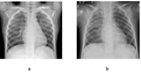
In this work, we trained the developed model on three datasets published by the Kaggle dataset. The three datasets were the result of digitizing medical images of the human body. The first dataset was the chest X-ray dataset1 representing data on a small amount of 5216 photos. The second was the Malaria dataset2, representing an intermediate amount of data, namely 27,560 pictures. The last was the PatchCam dataset3, which was a large dataset with a total of 220,025 images. The chest X-ray dataset [10] was a radiological image of human lungs categorized into two classes and not distributed proportionally, consisting of 3875 and 1341 for viral pneumonia/bacterial and normal ones. The entire picture had run through doctors’ labeling process and followed by an expert’s level of accuracy verification. Here are examples of a chest X-ray dataset in Figure 1.
1https://www.kaggle.com/paultimothymooney/chest-xray-pneumonia
2https://www.kaggle.com/miracle9to9/files1
3https://www.kaggle.com/c/histopathologic-cancer-detection
The malaria dataset was owned by the Open Knowledge Foundation4and pub- lished by the Kaggle dataset. Data was the result of digitization from the Thin Blood Smear process. The image was taken using an Android smartphone applica- tion integrated with a microscope using standard lighting. The data was distributed proportionally, with a total of 27,560 images. Experts carry out the labeling pro- cess by producing two categories of images, namely parasitized and normal. Here are examples image from the dataset in Figure 2.
Figure 1. X-ray dataset, (a) Normal and (b) bacterial/viral pneumonia.
Figure 2. Malaria dataset, (a) Normal and (b) parasitized.
Figure 3. PatchCam Dataset, (a) Cancerous and (b) non-cancerous.
4https://opendatacommons.org/licenses/by/1-0/index.html
The next dataset was the PatchCam Dataset [1, 19], published at the Kaggle competition. The data were small pathology images converted into digital for- mat, consisting of 220,025 images, and not evenly distributed in the two classes, cancerous and non-cancerous. Here are examples from the PatchCam dataset in Figure 3.
For the daily experiment, we used Google Collaboratory, and then the data were trained on a Dell Desktop with GEFORCE GTX 1060 6GB. Each code in this work was written in Python version 3.6 by exploiting jupyter notebook. Apart from that, the Tensorflow and Keras frameworks were also used in this work.
3. Methodology
3.1. Network architecture
In this work, we proposed an interconnected CNN model. This model was a combi- nation of three subnetworks consisted of three pretrained models. The purpose of combining the three subnetworks is to let the three subnetworks work independently in the training process to determine the influence of each subnetwork on decision making. Thus, the interconnected model will get the proper weight, increasing its ability in the classification task. The three subnetworks, namely, VGG19 consisted of sixteen convolution layers, InceptionV3 consisted of forty-eight layers of convo- lution, and MobileNet consisted of eighteen layers of convolution. The Multilayer Perceptron (MLP) of each subnetwork was replaced with three Fully Connected layers using the ReLU activation function to fit the interconnected models needed.
Before entering into MLP, the architectural design required a Flatten layer to con- vert the features’ dimensions. The next layer was the Concatenation layer, where the three output layers will be combined so that the interconnected model will only have one output. Afterward, the three Fully Connected layers were installed, consisting of two Fully Connected layers using the ReLU activation function and one Fully Connected layer using Soft-Max two classes to represent our dataset’s classification problem. Here it is shown the architectural design in Figure 4.
3.2. Training process
Due to variations between small and large datasets, the augmentation method [13] was employed to provide sufficient data for the model. The augmentation process that we have implemented includes rotation, shifting, shearing, zooming, and flipping. For simplicity purposes, a few aspects were standardized. We took 10% of the images from each dataset, then used them as a test set. Afterward, 70%
of the remaining images were allocated as a training set and 30% as a validation set. The input sizes of all datasets were set to 100×100 pixels. The batch sizes were set to 16 and an epoch of 50 for each training process.
In our work, emphasis is put on having a training process which is carried out simultaneously in a series of interconnections. Although each subnetwork has
Figure 4. Architecture of the interconnected Model.
authority in the training process, the training process is an integral part that cannot be separated from one and another. This process causes each subnetwork’s weights to be determined by the training process itself and not by the user. When a subnetwork has better performance than others, the subnetwork will automatically have more significant impact on the overall interconnected model. Conversely, if a subnetwork produces unsatisfactory performance, it will have less weight in the final decision process. In [7], the initial weights was determined to be equivalent for the three subnetworks. In our work, the interconnected model determined its weights according to the training process that each model gone through. The weighting process of each subnetwork was intervened neither at the initial nor during the final decision stage.
Utilizing the transfer learning method in the training process caused many layers that may not be necessary and will consume extra resources of the computational of our work. The Freezing layers technique as explained in [2] was implemented to save computation resources without destroying the model’s performance. The process includes freezing several layers causing the input images to go through these layers to avoid updating weights. This Freezing layers method aimed to diversify the three subnetworks, allowing three different perspectives to more effectively notice the image’s characteristics.
During the training process, the model tried to get the smallest possible Loss score to get the best possible Accuracy score. Thus, we aimed to minimize the Loss score of the model using the Soft-Max Loss function. The Soft-Max Loss
function itself was the product of implementing the Soft-Max function into the Loss function. To see the connection between these two functions more clearly, let’s look at the formula (3.1). As explained in [5, 16], the formula Soft-Max function 𝑓(𝑠) : R𝐾 → R𝐾 is a vector function in the range 0 to 1, where 𝐾 is number of classes.
𝑓(𝑠)𝑖= 𝑒𝑠𝑖
∑︀𝐾
𝑐=1𝑒𝑠𝑐. (3.1)
This formula is obtained by calculating the 𝑒number to the power of 𝑠𝑖, 𝑠𝑖 itself refers to the score𝑠from class 𝑖. Hence, the numerator divided by the sum of the constant𝑒to the power of all score in number of classes. So that when implemented into the Soft-Max loss function [5, 16] it will become:
𝐶𝐸=−
∑︁𝐾
𝑖
𝑡𝑖log(𝑓(𝑠)𝑖). (3.2) Equation (3.2) explains that cross-entropy𝐶𝐸 is the sum of ground truth𝑡𝑖 loga- rithm the CNN score of each class that represents by𝑓(𝑠)𝑖.
We were also optimizing our model by setting Adam optimizer at 1e-4 learning rate and decay 1e-6 for each subsequent epoch. Furthermore, we calculated the accuracy score based on the Confusion Matrix [3, 14], which results in True Positive (TP), True Negative (TN), False Positive (FP) and False Negative (FN). TP is representing ill patients as precisely predicted to be ill patients. Meanwhile, TN is healthy patients correctly predicted as healthy patients. On the other hand, FP is healthy patients incorrectly predicted as ill patients. and vice versa FN is ill patients, mistakenly classified as healthy patients. We also measured the Precision and Recall score to see the performance of the ill predicted label. For more details, the Accuracy, Precision, and Recall score calculation are in the equations. (3.3), (3.4), and (3.5).
Accuracy= TP+TN
TP+TN+FP+FN, (3.3)
Precision= TP
TP+FP, (3.4)
Recall= TP
TP+FN. (3.5)
4. Results
4.1. Training and validation accuracy
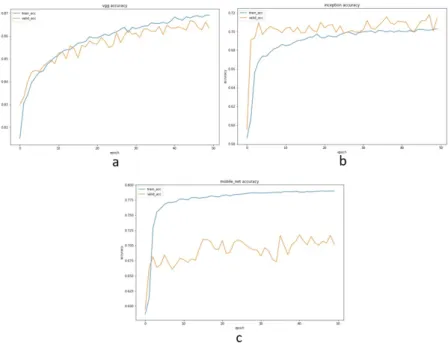
In the first experiment, the three subnetworks were trained separately. Thus each subnetwork provided its prediction result. The results from each subnetwork were then used in the voting process. Experiments using the chest X-ray dataset showed that the three pretrained models can be appropriately implemented. It can be ob- served from the ability of the three pretrained models to validate the training
results. The two intersecting lines in Figure 5 indicated that the training accuracy and the validation accuracy scores were comparable. It revealed that the three pre- trained models were suitable and did not overfit. Each model achieved a validation score of 0.91 for VGG19, 0.89 for InceptionV3, and 0.93 for MobileNet.
Figure 5. Training and validation accuracy for chest X-ray dataset:
a) VGG19, b) InceptionV3 and, c) MobileNet.
Likewise, the training process using the malaria dataset showed a good perfor- mance of VGG19 by achieving a validation score of 0.90. InceptionV3 and Mo- bileNet had satisfactory validation scores of 0.80 as shown in Figure 6.
For training the PatchCam dataset, VGG19 achieved optimum results in the classification task reported a score of 0.86 for validation accuracy. InceptionV3 showed satisfactory performance with a validation score of 0.70. The MobileNet pretrained model also achieved the same score with a small overfit condition. In Figure 7, the training and validation processes on the PathCam dataset were de- picted.
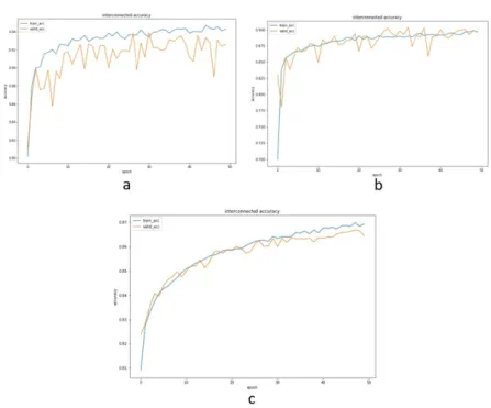
The training process for the interconnected model operated the same as the separate training process. The only difference was the interconnected model trains three submodels simultaneously. This model had trained all parameters owned by the three pretrained models. These experiments reported that the interconnected model showed comparable performance with any single model. The interconnected model’s validation accuracy scores compared to all single models are presented in Table 1.
Figure 6. Training and validation accuracy for malaria dataset:
a) VGG19, b) InceptionV3 and, c) MobileNet.
Figure 7. Training and validation accuracy for PatchCam dataset:
a) VGG-19, b) InceptionV3 and, c) MobileNet.
Figure 8. Training and validation accuracy of the interconnected model on all datasets: a) chest X-ray, b) Malaria, c) PatchCam.
Table 1. Validation accuracy of all models for three datasets.
Dataset VGG19 InceptionV3 MobileNet Interconnected
chest X-ray 0.91 0.89 0.93 0.93
Malaria 0.90 0.80 0.80 0.90
PatchCam 0.86 0.70 0.70 0.86
4.2. Visualization of training process
Figure 9 explains the steps that occur during the training process by visualizing [2] the images. Figure 𝑎represents the image that was input to the model. The original image size, as previously mentioned, was 100x100 pixels. Given that this dataset’s training process studied the completeness of photographs of human lungs, an example image from the normal category dataset is presented. Having the extracted features as shown in parts,𝑏to𝑑, then the part𝑒shows that the model can detect lungs in a healthy condition with an image representation showing the lungs appearing intact.
Figure 10 depicts the malaria dataset image from the input process, feature extraction, and object detection in human blood. Part𝑎is the image input to the model. Parts𝑏to𝑑are the extracted features by the models. Part𝑒is the model’s
Figure 9. a) Input, b)-d) Extracted Features, e) Heatmap.
heatmap as the classification result for the image labeled as malaria.
Figure 10. a) Input, b)-d) Extracted features, e) Heatmap.
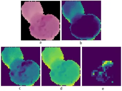
The training process on the PatchCam dataset aimed to detect the presence of cancer cells in the image. Therefore, when the image in Figure 11 𝑎was input to the model, the model performed the feature extraction process shown in Figure 11
𝑏 to𝑑. After that, the model can detect the cancer cells’ presence in the image as displayed in the heatmap in Figure 11𝑒.
Figure 11. a) Input, b)-d) Extracted Features, e) Heatmap.
4.3. Predicted results
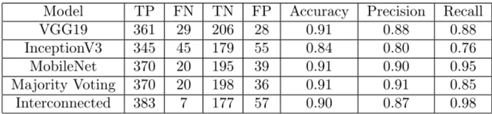
After training and validating all models on the dataset, The model was tested using the test set. This was performed to observe the model’s ability to predict new data. From the three pretrained models that we trained on the chest X-ray dataset, it can be reported that all models can predict the data accurately. Table 2 shows that all pretrained models achieved good accuracy scores, which were 0.91, 0.84, and 0.91 for VGG19, InceptionV3, and MobileNet, respectively. However, in this case, the interconnected model’s achievement has not exceeded majority voting performance, which can be seen from the majority voting accuracy score of 0.91. Nevertheless, the interconnected model results were comparable with both the single model and the majority voting. Table 2 also shows that the correctly and incorrectly predicted images is well distributed. The precision and recall score in Table 2 also indicates that the interconnected model’s ability was slightly better than the majority voting model. In retrieving images containing pneumonia, the interconnected model found 383 images with 7 images error or equivalent to a recall score of 0.98, compared to majority voting, with 370 images containing pneumonia and 20 images error or equivalent to 0.85 recall score. Even so, the two models’
precision score was comparable, namely, 0.91 for majority voting and 0.87 for the interconnected model.
A similar approach was applied to the malaria dataset to see the three models’
Table 2. Confusion matrix and classification report of chest X-ray dataset.
Model TP FN TN FP Accuracy Precision Recall
VGG19 361 29 206 28 0.91 0.88 0.88
InceptionV3 345 45 179 55 0.84 0.80 0.76
MobileNet 370 20 195 39 0.91 0.90 0.95
Majority Voting 370 20 198 36 0.91 0.91 0.85
Interconnected 383 7 177 57 0.90 0.87 0.98
ability to predict new data. Different results were obtained from this experiment, as shown in Table 3. This experiment gained an accuracy score for each pretrained model, consisting of 0.87 for VGG19, 0.87 for InceptionV3, and 0.72 for MobileNet.
The abilities MobileNet was not optimum because there was a significant error in predicting data in the positive class. In this experiment, the majority voting method cannot provide maximum results, namely 0.86 accuracy. On the other hand, the interconnected model can provide a proper weight, increasing the ac- curacy score to 0.88. Furthermore, the interconnected model showed satisfying performance on the positive class with a recall score of 0.82 compared to majority voting with a recall score of 0.74. This value represented the number of images identified with malaria that can be retrieved as many as 823 images with 177 errors for the interconnected model. In comparison, majority voting found 737 images with an error of 263 images. The Precision scores in Table 3 represent the level of precision of each model. It is shown that all models have a good level of precision, which is above 0.93.
Table 3. Confusion matrix and classification report of Malaria dataset.
Model TP FN TN FP Accuracy Precision Recall
VGG19 798 202 938 62 0.87 0.93 0.80
InceptionV3 776 224 963 37 0.87 0.95 0.78
MobileNet 443 557 997 3 0.72 0.99 0.44
Majority Voting 737 263 988 12 0.86 0.98 0.74
Interconnected 823 177 942 58 0.88 0.93 0.82
The last experiment utilized the PatchCam dataset. Comparing the three sub- network, the VGG19 model showed the best performance with an accuracy score of 0.87, followed by the InceptionV3 model with an accuracy score of 0.70, and the MobileNet with an accuracy score of 0.66. This experiment also produced one dominant model. Thus, the majority voting method did not work optimally and gained an accuracy score of 0.83. On the other hand, the interconnected model can provide a suitable weight for each model to get an accuracy score of 0.87. As seen in Table 4, the interconnected model has better Precision and Recall scores
than the majority voting. Thus the interconnected model has better performance in both classification classes, cancer and non-cancer images.
Table 4. Confusion matrix and classification report of PatchCam dataset.
Model TP FN TN FP Accuracy Precision Recall
VGG19 6692 2199 12400 709 0.87 0.89 0.75
InceptionV3 6638 2253 8838 4271 0.70 0.61 0.75
MobileNet 2696 6195 11882 1227 0.66 0.69 0.30
Majority Voting 5902 2989 12342 767 0.83 0.88 0.66 Interconnected 6721 2170 12316 793 0.87 0.89 0.77
5. Conclusions
After training all pretrained models separately and simultaneously on the three datasets, we concluded the interconnected model could be used when majority voting did not work optimally. The results can be seen in the second and third ex- periments using the Malaria and PatchCam dataset. Although the interconnected model’s accuracy score slightly corrected the score of majority voting, in predicting positive classes, the interconnected model worked better than other models on the three datasets. The interconnected model worked by giving the submodels the best weights without training them separately. This method was more efficient than first training of the three submodels to determine their abilities and then consider their appropriate weights.
Our work focused on the investigating of the interconnected model’s ability versus majority voting, but not analyzing the individual optimization of each sub- network’s architecture. It means that we used the transfer learning method without adjustment. This can be confirmed by comparing our work’s accuracy with sev- eral references which use the same dataset [11, 12, 15]. In this case, InceptionV3 and MobileNet’s pretrained models required adjustments in the depth and number of layers. Therefore, in our future work we will examine each network’s further optimization possibilities to help the developed system to be more accurate. In addition, the usage of the imbalanced dataset also influences the model’s perfor- mance. We consider using a method that can handle the imbalanced dataset’s problem to increase the model’s accuracy.
References
[1] B. E. Bejnordi,M. Veta, P. J. V. Diest,B. V. Ginneken, N. Karssemeijer, G.
Litjens, J. A. V. D. Laak, C. Consortium: Diagnostic assessment of deep learning algorithms for detection of lymph node metastases in women with breast cancer, JAMA 318.22 (2017), pp. 2199–2210.
[2] F. Chollet:Deep Learning With Pyhton, in: New York, USA: Manning Publication Co, 2018, p. 160.
[3] T. Fawcett:An Introduction to ROC Analysis, Pattern Recognition Letters 27.8 (2006), pp. 861–874,
doi:https://doi.org/10.1016/j.patrec.2005.10.010.
[4] D. Ganguly,S. Chakraborty,M. Balitanas,T.-h. Kim:Medical Imaging: A Review, in: International Conference on Security-Enriched Urban Computing and Smart Grid, Hei- delberg, Berlin: Springer, 2010, pp. 504–516,
doi:http://dx.doi.org/10.1007/978-3-642-16444-6_63.
[5] I. Goodfellow,Y. Bengio,A. Courville, in: Deep Learning, Cambrige MIT press, 2016, p. 181.
[6] S. Goswami,U. Dey,P. Roy,A. Ashour,N. Dey:Medical Video Processing: Concept and Applications, in: Feature Detectors and Motion Detection in Video Processing, IGI Global, 2017, pp. 1–17,
doi:http://dx.doi.org/10.4018/978-1-5225-1025-3.ch001.
[7] B. Harangi,A. Baran,A. Hajdu:Classification of skin lesions using an ensemble of deep neural networks, in: 2018 40th annual international conference of the IEEE engineering in medicine and biology society(EMBC), Honolulu, HI, USA: IEEE, 2018, pp. 2575–2578, doi:https://doi.org/10.1109/EMBC.2018.8512800.
[8] A. G. Howard, M. Zhu, B. Chen, D. Kalenichenko, W. Wang, T. Weyand, M.
Andreetto,H. Adam:MobileNets: Efficient Convolutional Neural Networks for Mobile Vision Applications, arXiv:1704.04861 (2017).
[9] H. Kasban,M. A. M. El-Bendary,D. H. Salama: A comparative study of medical imaging techniques, International Journal of Information Science and Intelligent System 4.2 (2015), pp. 37–58.
[10] D. Kermany,K. Zhang,M. Goldbaum:Labeled Optical Coherence Tomography (OCT) and Chest X-Ray Images for Classification, Mendeley Data v2.2,https://data.mendeley.
com/datasets/rscbjbr9sj/2, 2018,
doi:https://doi.org/10.17632/rscbjbr9sj.2.
[11] O. Lantang,A. Tiba,A. Hajdu,G. Terdik:Convolutional Neural Network for Predicting The Spread of Cancer, in: Proceedings of the 2019 10th IEEE International Conference on Cognitive Infocommunications (CogInfoCom), Naples, Italy: IEEE, 2019, pp. 175–180, doi:https://doi.org/10.1109/CogInfoCom47531.2019.9089939.
[12] Z. Liang,A. Powell,I. Ersoy,M. Poostchi,K. Silamut,K. Palaniappan,P. Guo, M. A. Hossain,A. Sammer,R. J. Maude,J. X. Huang,S. Jaeger,G. Thoma:CNN- Based Image Analysis for Malaria Diagnosis, in: 2016 IEEE Conference on Bioinformatics and Biomedicine (BBIM), Shenzhen, China: IEEE, 2016, pp. 493–496,
doi:https://doi.org/10.1109/BIBM.2016.7822567.
[13] A. Mikolajczyk,M. Grochowski:Data augmentation for improving deep learning in im- age classification problem, in: 2018 International Interdisciplinary PhD Workshop(IIPhDW), Swinoujście, Poland: IEEE, 2018,
doi:https://doi.org/10.1109/IIPHDW.2018.8388338.
[14] D. M. W. Powers:Evaluation: From Precision, Recall and F-measure to ROC, Informed- ness, Markedness and Correlation, Journal of Machine Learning Technologies 2.1 (2010), pp. 37–63,
doi:https://doi.org/10.9735/2229-3981.
[15] P. Rajpurkar,J. Irvin,K. Zhu,B. Yang,H. Mehta,T. Duan,D. Ding,A. Bagul, R. L. Ball, C. Langlotz, K. Shpanskaya, M. P. Lungren, A. Y. Ng: CheXNet:
Radiologist-Level Pneumonia Detection on Chest X-Rays with Deep Learning, arXiv preprint arXiv:1711.05225 (2017).
[16] P. Sadowski:Notes on back propagation,https://www.ics.uci.edu/pjsadows/notes. pdf (online) (2016).
[17] K. Simonyan,A. Zisserman:Very Deep Convolutional Networks for Large-Scale Image Recognition, arXiv preprint arXiv:1409.1556 (2014).
[18] C. Szegedy, W. Liu,Y. Jia,P. Sermanet, S. Reed,D. Anguelov,D. Erhan,V.
Vanhoucke,A. Rabinovich:Going Deeper with Convolutions, in: Proceedings of the 2015 IEEE Conference on Computer Vision and Pattern Recognition, Boston, MA, USA: IEEE, 2015, pp. 1–9,
doi:https://doi.org/10.1109/cvpr.2015.7298594.
[19] B. S. Veeling,J. Linmans,J. Winkens,T. Cohen,M. Welling:Rotation Equivariant CNNs for Digital Pathology, in: International Conference on Medical image computing and computer-assisted intervention, Springer, Cham, 2018, pp. 210–218.