Implicit Cost of the 2010 Foot-and-Mouth Disease in Korea

(1)

Introduction

Foot-and-Mouth Disease (FMD) is a highly contagious viral disease that affects cloven-hoofed animals such as cattle and swine. Animals with FMD typically have a high fever and blisters on the mouth, the mammary glands, and around the hooves (USDA APHIS, 2013). Affected animals will not die from FMD, but animals will be weakened and unable to produce meat and milk as before (USDA APHIS, 2013). FMD is transmitted directly through animal move- ment or indirectly through non-animal fomites or airborne transmission. An outbreak of FMD usually results in culling or killing affected animals (“stamping out”) and thus causes substantial economic losses in livestock sectors and related industries, such as the dairy and meat processing sectors.

Numerous research has addressed matters related with FMD outbreaks. Certain studies have evaluated different strategies to control the outbreak of an FMD incidence.

Garner and Lack (1995) investigated alternative control plans in Australia, using epidemiological simulation with an Input-Output (IO) model (explained in detail below).

They determined that destroying infected animals reduced the duration of the outbreak. Ekboir (1999) utilized similar IO modelling approaches and assessed the impact of a FMD outbreak in California (U.S.). Ekboir (1999) found that vaccination is the least expensive control strategy and that immediate migration is vital to stemming an outbreak.

Schoenbaum and Disney (2003) determined that effective control(s) of an FMD outbreak depend on herd demograph- ics and regional contact rates. Other studies such as Zhao et al. (2006), Jones (2010), and Kim et al. (2017) found that an improved animal traceability system may help to reduce the negative economic consequences of an FMD outbreak.

A different vein of research involves quantifying the economic impacts of an FMD outbreak. These studies used an IO model to measure the economic impacts of a hypothetical or simulated FMD outbreak. Lee et al. (2012)

estimated the economic impacts of a hypothetical agro- terrorism attack that made use of FMD pathogens. Pendell et al. (2007) also investigated a hypothetical impact of an FMD outbreak on the economy of southwest Kansas by using the Social Accounting Matrix approach, which is an extended IO model. Previously, Caskie et al. (1999) had used an IO model to quantify the economic effects of a BSE- induced reduction of livestock for Northern Ireland. More recently, Schroeder et al. (2015) also utilized the IO framework for evaluating the effect of a high-capacity emergency vaccination during an FMD outbreak.

Studies that measure the effects from an actual FMD outbreak include Scudamore (2002) and Thompson et al. (2002) for a case in the United Kingdom (UK). In 2001, the UK experienced a severe FMD outbreak. At least 57 premises were infected by the time the first case was identified in Feb- ruary of that year (Scudamore, 2002). By September 2001, over 6 million animals had been killed and the disease had spread to Ireland, France and the Netherlands (Scudamore, 2002). Thompson et al. (2002) estimated economic losses from the FMD incidence in the UK to be between 10.7 billion US dollars to 11.7 billion US dollars. The 2010-2011 FMD outbreaks in Korea were severe and caused large economic effects on livestock sectors and related industries in Korea. The number of culled animals were upwards of 3.5 million heads from November 2010 to April 2011. More than 90% of the culled animals were swine (3.3 million heads) (KREI, 2011, Table 3-18, pp. 147-148). Using the IO model, KREI (2011) estimated the economic impact due to FMD outbreak in 2010 to be more than 4 trillion Korean Won (≈ 3.6 billion US dollars) (KREI, 2011, p. 283).

The economic impacts from animal disease like FMD can be divided into three categories. First, the “direct impacts” are from the reduction in animal production due to culling/killing animals. Second, the “indirect impacts” are from changes in inter-industry transactions as they respond to the affected livestock industry; for example, losses in dairy and meat processing sectors; and third, the “induced effects” which are the decreases in household income Man-Keun KIM* and Hernan A. TEJEDA**

Implicit Cost of the 2010 Foot-and-Mouth Disease in Korea

The most destructive foot-and-mouth disease (FMD) outbreak in Korea occurred in November 2010. Various studies have quantified the economic impact of culling affected animals, mostly swine, from the event by applying different assumptions to the Input-Output (IO) model. The present study takes into account a type of implicit cost, considering the types of effects in the previous literature, as well as costs that have been unaccounted for in prior studies. A seasonal autoregressive model (SARIMA) is estimated employing the number of swine slaughtered leading up to the 2010 FMD outbreak, and forecasts from the model are compared to the actual drop and rebound. The unaccounted implicit cost is estimated to be more than 2 trillion Korean Won (≈ 1.8 billion US dollars), which is a cost Korea must give up or cannot recover. This study serves to strengthen the justification of applying preventive efforts to reduce the likelihood and economic impact of an animal disease outbreak and may be applied in other countries.

Keywords: Foot-and-Mouth Disease (FMD), Implicit cost, Seasonal autoregressive integrated moving average (SARIMA) JEL classifications: Q11; Q13; R15

* Department of Applied Economics, Utah State University. Logan, Utah 84322, USA. Corresponding author: mk.kim@usu.edu

** Twin Falls Research and Extension Center, University of Idaho, Twin Falls, Idaho 83301, USA.

Received: 10 January 2018; Revised: 24 April 2018; Accepted: 14 May 2018.

(2)

generated from the direct and indirect effects.¹ Input-Output (IO) analysis measures these impacts using IO multipliers (Miller and Blair, 2009). Moon et al. (2013b) analysed the multiplier effects of FMD outbreaks in 2000, 2002, and 2010 using the Korean IO model. They estimated the total economic impact of FMD outbreak in Korea in 2010 to be 3.5 trillion Korean Won (≈ 3.2 billion US dollars). KREI (2011) also estimated the economic impact due to FMD outbreak in 2010 to be more than 4 trillion Korean Won (≈ 3.6 billion US dollars) using a similar approach. KREI (2011) and Moon et al. (2013b) estimated the economic impacts from FMD outbreak using a standard demand-driven IO model in situations where the FMD outbreak alters the final demand.

Kim (2015) suggested a supply-driven IO approach because the FMD outbreak alters livestock production, i.e., supply, not the final demand. Kim (2015) estimated these economic impacts to be 7.6 trillion Korean Won (≈ 6.8 billion US dollars) which is substantially higher than the other two studies.

As Pendell et al. (2007) and Kim (2015) pointed out, the FMD outbreak in the UK confirmed the need to investigate and understand the economic impacts of these FMD events, in order to develop effective public policies that abate the effects from these outbreaks. In the case of Korea, KREI (2011), Moon et al. (2013b), and Kim (2015) reported the economic impacts of the 2010 FMD outbreak in Korea using the IO framework as well. Preventive controls of the animal disease outbreaks are important to help mitigate economic losses from such outbreaks. As discussed in previous studies, an animal disease like FMD may cause severe economic impacts. Moreover, as food supply chains have become increasingly global, the impact on international trade of a potential FMD outbreak has grown to be a major concern for livestock exporters (Park et al. 2008). Export countries have a vital interest in maintaining FMD-free status to maintain trade relationships.

Where preventive controls of animal disease outbreaks are concerned, African Swine Fever (ASF) should receive close attention, especially in Europe given its geographic proximity. ASF is an endemic and highly contagious haem- orrhagic disease of swine (Beltrán-Alcrudo et al. 2017).

ASF is currently widespread in sub-Saharan Africa, Eastern Europe and the Italian island of Sardinia. With the increased transmission of ASF, there is growing global concern that the virus may spread further into other regions (Beltrán-Alcrudo et al. 2017). Since 2015-2016, ASF has maintained its pres- ence and continues to spread throughout Russia, the Ukraine, Estonia, Latvia, Lithuaia and eastern Poland (USDA FAS, 2016). As such, the present investigation offers pertinent inferences for the European region. As emphasized in this study, the economic costs of the outbreak may actually be higher when the unaccounted cost is taken into considera- tion.

This research begins with a question regarding the implicit costs of “actual” livestock diseases like the 2001 FMD event in the UK and 2010 FMD event in Korea. In particular, we study the more recent 2010 FMD outbreak in Korea and its effect on

1 We may add derived costs such as governmental expenditure/subsidies and environmental degradation from the carcass burial construction. Kim and Kim (2013) estimated the cost of environmental degradation from the carcass burial and sites construction.

the country’s main livestock industry – swine. This outbreak led the the United Nations Food and Agriculture Organiza- tion (FAO) to issue a call for increased global surveillance.

Our approach is also applicable to measuring the effects from other actual or hypothetical major disease outbreaks. We use the term implicit cost in this paper to refer to the unaccounted economic cost, i.e., type of opportunity cost. Perhaps the term persistent costs would make better sense since the impact of the 2010 FMD outbreak was persistent for several months after the FMD had been contained. As described previously, explicit costs are the economic costs taken into account as a result of the damage from the FMD incident. These accounted costs are from the direct, indirect, and induced effects of culling the animals in response to the FMD outbreak. Con- versely, the implicit cost or persistent cost is an unaccounted cost which can be estimated by comparing the level of livestock slaughtered under FMD outbreak (i.e., “the treatment group”) to the number of livestock slaughtered without FMD outbreak (i.e., “a control group” or counterfactual scenario with no FMD). In doing so we estimate a cost equal to what we must give up (i.e. cannot recover) as a consequence of the FMD outbreak, which also includes unaccounted indirect and induced costs. We can estimate implicit indirect and induced costs using Input-Output framework as well.

Unfortunately, it is impossible to find a valid control or counterfactual situation because the FMD outbreak in 2010 occurred everywhere in Korea. Given the difficulties associated with obtaining a valid control group, time series methods are applied, specifically a seasonal autoregressive- moving average (SARIMA) model is used to estimate the counterfactual number of livestock slaughtered. Focusing on the swine sector in Korea, we find that between March 2011 and October 2011, the accumulative difference in the number of swine slaughtered was estimated to be a bit more than 2 million heads. The approximated implicit or unaccounted direct implicit cost of FMD is 1.06 trillion Korean Won (≈ 0.95 billion US dollars) assuming the average swine price received by farmers in 2011 to be 328,000 Won/110kg (≈ 295 US dollars/110kg). The implicit or unaccounted indirect and induced costs from this are also estimated to be 1.41 trillion Korean Won (≈ 1.27 billion US dollars) and 0.66 trillion Korean Won (≈ 0.59 billion US dollars), respectively;

by using the standard IO multipliers from Bank of Korea (2014). Thus, the total implicit cost is estimated to be 3.14 trillion Won (≈ 2.83 billion US dollars), which is the cost Korea must give up due to the persistent FMD outbreak.

This paper contributes to the literature on estimating the effects of livestock disease in a regional economy, where up to date there is no study addressing the implicit cost of livestock disease outbreak. Thus, we seek to identify unaccounted economic effects of a major disease outbreak affect- ing a significant agricultural sector, by applying a different approach that permits to estimate and determine these (additional) omitted costs. This new study serves to strengthen the justification of applying preventive efforts to reduce the likelihood and the economic impact of an animal disease outbreak. The swine sector in Korea is studied in order to estimate the implicit cost of the FMD outbreak in 2010.

This paper consists of four sections. Section 2 explains the data used and provides explanations of the method. Section

(3)

3 contains the empirical results and policy implications and section 4 has remarks and concludes the paper.

Data and methodology

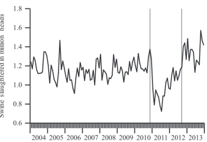
The number of swine slaughtered is taken from the Record of Livestock Slaughter, Animal and Plant Quaran- tine Agency, which are archived by the Korean Ministry of Agriculture, Food and Rural Affairs (each year). We compiled monthly data from January 2004 to December 2013 (132 observations). The data series is plotted in Figure 1.

The number of swine slaughtered substantially decreased immediately following the FMD outbreak (November 2010 as indicated by the first grey vertical line in Figure 1) due to culling affected swine. The actual reduction in the number of swine slaughtered between the fourth quarter of 2010 (sum of number of swine slaughtered between October 2010 and December 2010) and the first quarter of 2011 (sum of number of swine slaughtered between January 2011 and March 2011) was 1.24 million heads. The number of swine slaughtered has steadily rebounded after the FMD outbreak.

It seems to reach the level prior to the FMD in October 2012 (the second grey vertical line in Figure 1).

The autoregressive-moving average (ARMA) models use lags and shifts in the data to uncover patterns and predict the future values. Box and Jenkins (1976) discussed the general ARMA models. The autoregressive (AR) part of the model involves regressing the variable on its own lagged values and the moving average (MA) part involves modelling the error term as a linear combination of current and past error terms.

Note that most of discussions regarding ARMA modelling in this article follows Lütkepohl and Krätzig (2004) closely including notations.

The model is referred to as ARMA(p,q) where p is the order of the AR part and q is the order of MA part as in equation (1)²:

(1) where y_t is a stationary time series data and ɛ_t is the error term which is distributed independent identically, i.e., ε_t~ iid (0, σ²). Using the lag operators, where L^ky_t= y_t–k, equation (1) can be rewritten as

ϕ(L)y_t= θ(L)ε_t (2)

where here ϕ(L) = 1 – ϕ₁L – ϕ₂ L² – ··· – ϕ_p L^p and θ(L) = 1 + + θ₁L + θ₂L²+ ··· + θ_q L^q.

The (non-seasonal) ARIMA models are extensions of the ARMA model, where here y_t is nonstationary (integrated), and where an initial differencing step is applied to convert the data into being stationary. Non-seasonal ARIMA models are denoted ARIMA(p,d,q) where parameter d is the degree of differencing³:

2 ARMA(1,1), for example, is written as y_t = ϕ₁y_t–1 + ε_t + θ₁ε_t–1 or (1 – ϕ₁L) y_t =

= (1 + θ₁L) ε_t.

3 ARIMA(1,1,1), for example, is given by ∆y_t = ϕ₁∆y_t–1 + ε_t+ θ₁εt–1 or (1 – ϕ₁L)∆y_t=

= (1 + θ₁L)ε_t.

ϕ(L) ∆^d y_t= θ(L) ε_t (3)

The seasonal ARIMA (SARIMA) models are formed by including additional seasonal terms (e.g. s = 12 for monthly data) and is denoted by SARIMA(p,d,q)(P,D,Q)_s, where s refers to the number of periods in each season and the upper case P, D, and Q refers to the autoregressive, differenc- ing, and moving average terms for the seasonal part of the ARIMA model⁴:

(4) where ϕ(L) = 1 – ϕ₁L – ϕ₂L² – ··· – ϕ_p L^p; ϕ_s (L^s) = 1 – ϕ_s1 L^s– – ··· – ϕ_sP L^sP; θ(L) = 1 + θ₁ L+θ₂ L²+ ··· + θ_q L^q; and θ_s (L^s ) = 1 + θ_s1 L^s+ ··· + θ_sQ L^sQ. In other words, in addition to the regular AR and MA operators, there are operators in seasonal powers of the lag operator. Note that in practice, deterministic terms may added to equations (1) to (4) such as constant term and/or a trend.

For the purpose of this study, the first 83 observations (from January 2004 to November 2010) are utilized to estimate the SARIMA model to forecast the number of swine slaughtered after the FMD outbreak for the following 25 months (i.e., till December 2012). We then compare the forecasted number of swine slaughtered (“counterfactual”) with the actual number of swine slaughtered.

The order of first differencing, represented by the value d in SARIMA(p,d,q)(P,D,Q)_s, is determined according to a non-stationary test, specifically the Augmented Dickey- Fuller (ADF) test (Dickey and Fuller, 1979) and the KPSS test (Kwiatkowski et al., 1992) explained in the following section. The order of seasonal differencing, represented by the value of D, is determined by applying the HEGY test (Hylleberg, et al., 1990), once again described in the fol- lowing section. The optimal combination for the values of p, q, P, and Q are determined by minimizing certain loss

4 For example SARIMA(1,1,1)(1,0,1)₄ model is given by (1 – ϕ₄₁L⁴)(1 – ϕ₁L)∆y_t=

= (1 + θ_s1L⁴)(1 + θ₁L) ε_t or ∆yt = ϕ₁ ∆yt–1 + ϕ₄₁ y_t–4 – ϕ₁ϕ₄₁∆yt–5 + εt + θ₁ εt–1 + θ_s1εt–4 + + θ₁θ_s1ε_t–5.

0.6 0.8 1.0 1.2 1.4 1.6 1.8

2004 2005 2006 2007 2008 2009 2010 2011 2012 2013

Swine slaughtered in million heads

Figure 1. Monthly number of swine slaughtered and 2010 FMD outbreak.

Note: First grey vertical line – FMD outbreak (November 2010); second grey vertical line – the number of swine slaughtered seems to reach the level prior to FMD outbreak.

Source: Animal and Plant Quarantine Agency, Korean Ministry of Agriculture, Food, and Rural Affairs.

(4)

function(s); for example, Akaike information criterion (AIC) or Bayesian information criterion (BIC).

Estimation and forecasting

The purpose of identification is to transform the nonstationary time series into a stationary series by differencing, if necessary. As shown in Figure 1, however, the number of swine slaughtered until November 2010 seems to be stationary without a trend even though there might exist some degree of seasonality. As mentioned before, the first 83 observations (from January 2004 to November 2010) are utilized to estimate the SARIMA model. To observe the stationarity of the series, ADF⁵ and KPSS⁶ tests on the number of swine slaughtered are conducted and results are reported in Table 1. As shown in Table 1, both tests confirm that the number of swine slaughtered is stationary, i.e., d = 0.

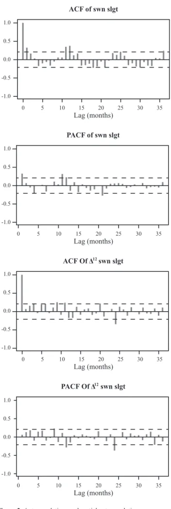
To see if there exists any seasonality, the autocorrelation functions (ACF) and the partial autocorrelation functions (PACF) for the series are plotted in the first row of Figure 2.

The ACF has a significant spike at lag 1 which suggests non- seasonal MA(1) component. Also, a significant spike at lag 11 (and 12) in the ACF suggests seasonal MA(1) component.

There might be AR(1) component because the PACF plot has a significant spike at lag 1. The ACF and the PACF are plotted for the series after performing a seasonal difference, i.e.,

∆¹²y_t = y_t – y_t–12 and presented in the second row of Figure 2. The ACF and PACF here indicate that there exists a clear seasonal MA(1) component in the model.

Table 1: Non-stationarity tests for the number of swine slaughtered from Jan 2004 to Nov 2010.

Raw data ADF test

(non-zero mean) KPSS Test (level stationary)

Test stat. -4.409 0.197

Lags^a 1 3

5% critical value -2.89 0.463

Decision^b Reject null Fail to reject null

S S

a Lags for ADF test is determined by minimizing BIC and for KPSS test is given by Newey-West lags, , where T is the number of observations

b ADF test - testing the null hypothesis of nonstationarity, thus the series is stationary by rejecting null hypothesis, KPSS test - testing the null hypothesis of stationarity, thus the series is stationary by failing to reject null hypothesis, and NS = nonstationary, S = stationary.

Source: authors’ calculation; critical values are taken from Davidson and MacKinnon (1993)

To check for the existence of the seasonal unit root (whether D = 0 or not), the HEGY test (Hylleberg, et al., 1990) is performed. The HEGY test was originally devel- oped for quarterly data, and was extended for the monthly data by Franses (1991), and Beaulieu and Miron (1993).

The HEGY test for monthly data is based on the following regression as explained in Rodrigues and Osborn (1999):

5 To compute the test statistics, we fit the regression,

, via least squares and test H₀: β = 0 against H_A:β < 0.

6 The KPSS test is based on the regression, y_t = r_t + e_t, that breaks up a series into a random walk and a stationary error (e_t). If the variance is zero,

, then r_t = r₀ for all t meaning that y_t is stationary.

0 -0.5 -1.0 0.0 0.5 1.0

5 10 15 20 25 30 35

ACF of swn slgt

Lag (months) PACF of swn slgt

0 -0.5 -1.0 0.0 0.5 1.0

5 10 15 20 25 30 35

Lag (months) ACF Of Δ swn slgt¹²

0 -0.5 -1.0 0.0 0.5 1.0

5 10 15 20 25 30 35

Lag (months) PACF Of Δ swn slgt¹²

0 -0.5 -1.0 0.0 0.5 1.0

5 10 15 20 25 30 35

Lag (months)

Figure 2: Autocorrelations and partial autocorrelations.

Source: authors’ calculation

(5)

where x_i,t–1 are linear transformation of lagged values of y_t (see Beaulieu and Miron, 1993, page 308, for the list of

x_i,t–1). The null hypothesis implies that π₁ = 0, π₂ = 0, π_k–1 =

π_k = 0 for k = 4,6,8,10,12 (joint F test) (Rodrigues and Osborn, 1999). To control the overall level of significance for the aforementioned null hypotheses, Taylor (1998) added the null hypotheses, π₁ = ··· = π₁₂ = 0 and π₂ = ··· = π₁₂ = 0.

Results are reported in Table 2. As shown in Table 2, there is no seasonal unit root and, therefore, D = 0.

Identification steps discussed in identification section suggests d = 0 (series is stationary) and D = 0 (series doesn’t have seasonal unit root). The ACF and the PACF suggest non-seasonal MA(1), seasonal MA(1), and non-seasonal AR(1) components. All told, the initial candidate model is SARIMA(1,0,1)(0,0,1)₁₂. We estimated different specifications (Table 3). As shown in Table 3, the final model is SARIMA(1,0,0)(0,0,1)₁₂ which has the minimum value of BIC. The estimation result is in Table 4 with standard errors in parentheses.

A portmanteau test is performed after estimating the model in Table 4 to confirm that the residuals from SARIMA(1,0,0)(0,0,1)₁₂ are uncorrelated. If there are cor- relations between residuals, then there is information left in the residuals (Hyndman and Athanasopoulos, 2013). The Ljung-Box⁷ test confirms that the residuals are uncorrelated (test statistics = 14.38 and p-value = 0.28 when lag = 12).

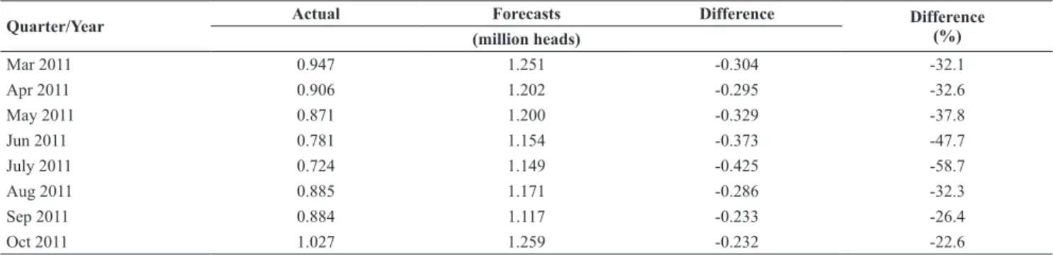
The SARIMA model in Table 4 is used to forecast the number of swine slaughtered for periods after the FMD outbreak, covering from December 2010 to December 2012. The predicted values are subsequently compared to the actual values. Figure 3 shows the sequence of forecasts (solid grey line) for the number of swine slaughtered each month, including its 95% confidence interval (dotted grey lines), and the actual number of swine slaughtered (dark line). Note that the forecasts of future values will eventu- ally converge to the mean and stay there because the number of swine slaughtered is a stationary process (see Table 1) as shown in Figure 3.

Actual values, estimated (forecasted) values, the difference of them and the percentage of difference are reported in Table 5. Note that this difference in the number of swine slaughtered between December 2010 and February 2011 should be considered as the explicit cost. As indicated in KREI (2011, page 53 and Figure 2-3), the FMD outbreak occurred on November 28, 2010 and the number of affected animals increased very fast until the end of January 2011. The number of newly affected animal was one head per day in February 2011 once the second vaccination was completed.

The reduction of swine slaughtered between December 2010 and February 2011 is removed from the calculation of the implicit cost, which consists of the accounted or explicit cost. We use the term implicit cost in the paper to refer to the unaccounted economic impact that is persistent after con- taining the FMD outbreak at the end of February 2011.

7 The Ljung-Box test is based on , where r_k is the autocorrelation for lag k and T is the number of observations. Large values of Q suggest that the autocorrelation do not come from a white noise series (Ljung and Box, 1978).

Table 2: Seasonal unit root test for number of swine slaughtered between Jan 2004 and Nov 2010.

Null

hypothesis Test

Stat p-value Decision at 10%

π₁ = 0 -1.100 0.629 Fail to reject A unit root exists π₂ = 0 -2.199 0.019 Reject No unit root exists π₃ = π₄ = 0 1.052 0.341 Fail to reject A unit root exists π₅ = π₆ = 0 1.836 0.155 Fail to reject A unit root exists π₇ = π₈ = 0 2.413 0.087 Reject No unit root exists π₉ = π₁₀ = 0 5.772 0.004 Reject No unit root exists π₁₁ = π₁₂ = 0 4.642 0.011 Reject No unit root exists π₁ = π₂ = ··· = π₁₂ 3.446 0.014 Reject No unit root exists π₂ = ··· = π₁₂ 3.611 0.005 Reject No unit root exists Note: Constant is included in equation (5). Other specifications are possible such as adding seasonal dummies (not reported here to save space). Results are available upon request. In case of adding seasonal dummies, we fail to reject the null hypothesis only for the first case, π₁ = 0, and reject all other null hypotheses.

Table 3: SARIMA model and values of Bayesian Information Criteria.

Model BIC

SARIMA(1,0,1)(0,0,1)₁₂ (Initial candidate) -148.05

SARIMA(0,0,1)(0,0,1)₁₂ -150.42

SARIMA(10,1)(0,0,2)₁₂ -143.78

SARIMA(1,0,1)(1,0,1)₁₂ -143.78

SARIMA(1,0,0)(0,0,1)₁₂ (final model) -151.63

SARIMA(1,0,2)(0,0,1)₁₂ -144.76

Table 4: SARIMA(1,0,0)(0,0,1)₁₂ regression result.

Coefficient Std. Err.

Non-seasonal AR(1) 0.2554^*** (0.1023)

Seasonal MA(1) 0.5631^*** (0.1244)

Constant 1.1675^*** (0.0204)

σ_ε 0.0849^*** (0.0061)

No. obs. 83

Log likelihood 84.65

BIC -151.63

Note: The test of the variance against zero is one sided Source: authors’ calculation

0.6 0.8 1.0 1.2 1.4 1.6 1.8

2012 2011

2010 2009

2008

Swine slaughtered in million heads

Figure 3: Actual and forecasted number of swine slaughtered.

Dark line = actual number of swine slaughtered; Grey line = forecasted number of swine slaughtered; Dotted line = 95% confidence bands

Source: actual number of swine slaughtered is compiled from Animal and Plant Quar- antine Agency, Korean Ministry of Agriculture, Food, and Rural Affairs; forecasted number of swine slaughtered is calculated using SARIMA estimates in Table 4.

(6)

Between March 2011 and October 2011, the loss in the number of swine slaughtered due to the persistent FMD outbreak is approximately 2.17 million heads (between 0.95 million heads ~ 3.4 million heads). We consider October 2011 as the end of forecasting horizon, and compute the loss in the number of swine slaughtered, because the actual number slaughtered rebounded up and reached the lower 95%

confidence level in October 2011. The difference between the actual and forecast values still exist after October 2011, but it is not evident that this may be solely because of the FMD outbreak.

Note that Korea-EU Free Trade Agreement (FTA) has been provisionally applied since July 2011 (and formally ratified in December 2015), which may have increased pork imports from the EU due to the lowered tariff; and in turn, potentially have affected the number of swine slaughtered.

In other words, the loss in the number of swine slaughtered during August-October 2011 might be overestimated. Pork imports from the EU increased by 50%, to 208,271 tons in 2011 from 139,343 tons in 2010 (Table 3 in Han et al., 2016).

Perhaps this increase in pork imports is partly because of the 2010 FMD outbreak and also partly because of Korea-EU FTA. Unfortunately, it is very difficult to distinguish among these two possible causes. We argue that a sharp increase in pork imports from the EU in 2011 responded more to the late November 2010 FMD outbreak, rather than to the July 2011 Korea-EU FTA, for the following two reasons.

First, pork imports from the EU in 2012 (second calendar year of Korea-EU FTA, or its first full year of FTA imple- mentation) decreased to prior 2010 levels, that is, 125,446 tons. Moreover, pork imports in 2013 (third calendar year of Korea-EU FTA, or its second full year of FTA implemen- tation) reached 148,558 tons (Table 3 in Han et al., 2016), which was after the swine inventory had rebounded. Second, pork is the most sensitive product in the FTA and it has a 10-year transition period until having duty free access. The tariff rate before FTA was 25% for frozen pork belly and 22.5% for fresh pork belly, which means that the tariff rate in 2011 was 22.7% for frozen pork belly and 20.4% for fresh pork belly (Moon et al., 2013a). Thus, the drop-in tariff rate impact for 2011 from the FTA would be minimal, if any. In addition, Moon et al. (2013a) indicate that “… 2010 FMD outbreak has resulted in a sharp increase in pork imports from the EU… and pork imports from the EU decrease in the second year, after domestic supply has recovered …” (Moon et al., 2013a, page 5).

Table 5: Actual and forecasting values of number of swine slaughtered after FMD outbreak.

Quarter/Year Actual Forecasts Difference Difference

(million heads) (%)

Mar 2011 0.947 1.251 -0.304 -32.1

Apr 2011 0.906 1.202 -0.295 -32.6

May 2011 0.871 1.200 -0.329 -37.8

Jun 2011 0.781 1.154 -0.373 -47.7

July 2011 0.724 1.149 -0.425 -58.7

Aug 2011 0.885 1.171 -0.286 -32.3

Sep 2011 0.884 1.117 -0.233 -26.4

Oct 2011 1.027 1.259 -0.232 -22.6

Source: actual number of swine slaughtered is compiled from Animal and Plant Quarantine Agency, Korean Ministry of Agriculture, Food, and Rural Affairs; forecasted number of swine slaughtered is calculated using SARIMA estimates in Table 4.

To estimate the implicit cost of 2010 FMD in Korea, the loss in the number of swine slaughtered is multiplied by the average swine price received by farmers in 2010 (mostly before the FMD outbreak), which was 328,000 Won/110kg (≈ 295 US dollars/110kg) (eKAPEPIA price information, Korea Institute for Animal Products Quality Evaluation (KAPE)). According to eKAPEPIA (http://www.ekapepia.

com/637.su) the swine price received by farmers had not varied much during the years 2008-2010. However, swine prices increased substantially after the FMD outbreak, to more than 480,000/110kg (≈ 432 US dollars/110kg). We conjecture that the swine price received by farmers would not have changed substantially in the first quarter of 2011 if the FMD outbreak had not occurred in November 2010.

As a result, the estimated implicit direct cost of FMD is 713 ± 402 billion Korean Won ( 642 ± 362 million US dollars). Implicit indirect and induced economic impacts can be computed using the standard Input-Output multipliers as in KREI (2011) and Moon et al. (2013b). The implicit indirect cost is estimated to be 947 ± 534 billion Korean Won (≈ 852

± 481 million US dollars) using the standard IO multipliers for the swine sector from Bank of Korea (2014). The implicit induced cost is estimated to be 447 ± 252 billion Korean Won (≈ 402 ± 176 million US dollars). As such, the total implicit cost is estimated to be 2,107 ± 1,189 billion Korean Won (1,896 ± 1,070 million US dollars). As discussed, this is the cost Korea must give up, or cannot recover, due to the FMD outbreak.

Concluding remarks

This research begins with a question regarding the implicit cost (persistent cost) of livestock disease, focusing on 2010 FMD outbreak in Korea. These implicit costs can be estimated by comparing the level of livestock slaughtered during a FMD outbreak (i.e., “the treatment group”) to the number of livestock slaughtered if there is no FMD outbreak (i.e., “a control group” or counterfactual scenario of no FMD). In doing so we estimate the cost equal to what we must give up because of the FMD outbreak. Given the difficulties associated with identifying a control group, we use the seasonal autoregressive-moving average to estimate counterfactual number of livestock slaughtered. The focus of the study is on the swine sector in Korea, and find that up to October 2011, the accumulative difference in the number of

(7)

swine slaughtered was estimated to be more than 2 million head. The approximated implicit direct cost of FMD is 713 billion Korean Won (≈ 642 million US dollars). The implicit indirect and induced cost from this are estimated to be 947 billion Korean Won (≈ 852 million US dollars) and 447 billion Korean Won (≈ 402 million US dollars), respectively; by using the standard IO multipliers for the swine sector from Bank of Korea (2014). The total implicit cost is estimated to be 2,107 billion Korean Won (1,896 million US dollars).

This paper contributes to the literature on quantifying the effects of livestock disease in a regional economy where there is no study up to this date regarding the implicit cost of a livestock disease outbreak. The swine sector in Korea is analysed to estimate the implicit cost of the FMD outbreak in 2010. Results consider economic losses that were not previously accounted for. This study serves to strengthen the justification of applying preventive efforts to reduce the likelihood and economic impact of an animal disease outbreak. In addition, the study’s approach is applicable to other hypothetical or actual cases of potential disease outbreaks, as is the plausible case of ASF in Europe.

Suggesting policy options to mitigate negative economic impacts of the FMD outbreak may be beyond the scope of this study. However, livestock and meat traceability system may be a way to improve preventive controls of the animal disease outbreak. Animal and meat traceability as a man- datory system would have been useful to track livestock movements in a pertinent country or region (e.g. EU) by establishing an identification number for premises where livestock were located, assigning animals an identification number (either individual or group), and implementing a national, electronic database for livestock tracking. It has been supported by the animal health community (Kim et al., 2017; Bailey, 2007; Bailey and Slade, 2004; Lawrence, 2004) who have viewed such a system as being an important component for tracking, controlling, and eradicating animal disease outbreaks.

References

Bailey, D. (2007): Political Economy of the U.S. Cattle and Beef Industry: Innovation Adoption and Implications for the Future.

Journal of Agricultural and Resource Economics 32 (3): 403- 416. https://doi.org/10.1080/01436590701192744

Bailey, D., and Slade, J. (2004): Factors Influencing Support for a National Animal Identification System for Cattle in the United States. Economic Research Institute Study Paper 283. Depart- ment of Economics, Utah State University. May.

Bank of Korea (2014): 2010 Input-Output Statistics. Seoul, Korea.

Beltrán-Alcrudo, D., Arias, M., Gallardo, C., Kramer, S. and Pen- rith, M.L. (2017): African Swine Fever: Detection and Diagno- sis – A Manual for Veterinarians. FAO Animal Production and Health Manual No. 19. Rome. Food and Agriculture Organiza- tion of the United Nations (FAO).

Box, G.E. and Jenkins, G.M. (1976): Time Series Analysis: Fore- casting and Control. Holden-Day, San Francisco, U.S.

Beaulieu, J.J. and Miron, J.A. (1993): Seasonal Unit Roots in Aggregate U.S. Data, Journal of Econometrics 55, 305-328.

https://doi.org/10.1016/0304-4076(93)90018-Z

Caskie, P., Davis J. and Moss, J.E. (1999): The Economic Impact of BSE: A Regional Perspective. Applied Economics 31, 1623- 1630. https://doi.org/10.1080/000368499323148

Davidson, R. and MacKinnon, J. (1993): Estimation and Inference in Econometrics. Oxford University Press; 1 edition, 896 pages.

Dickey, D. A. and Fuller, W. A. (1979): Distribution of the Estima- tors for Autoregressive Time Series with a Unit Root, Journal of the American Statistical Association 74, 427-431. https://doi.

org/10.1080/01621459.1979.10482531

Ekboir, J.M. (1999): Potential Impact of Foot-and-Mouth Disease in California: The Role and Contribution of Animal Health Sur- veillance and Monitoring Services. Agricultural Issues Center, University of California, Davis.

Franses, P.H. (1991): Seasonality, Nonstationarity and Forecasting of Monthly Time Series, International Journal of Forecasting 7, 199-208. https://doi.org/10.1016/0169-2070(91)90054-Y Garner, M.G., and Lack, M.B. (1995): An Evaluation of Alternative

Control Strategies for Foot-and-Mouth Disease in Australia:

A Regional Approach. Preventive Veterinary Medicine 23, 9-32. https://doi.org/10.1016/0167-5877(94)00433-J

Han, S, Nam, K. and Jeong, H. (2016): Impacts and Implications of Korea-EU FTA to Agricultural Sector after 5 Years of Effectua- tion. Agricultural Policy Focus No. 127, Korea Rural Economic Institute (KREI). [In Korean]

Hyndman, R.J. and Athanasopoulos, G. (2013): Forecasting: Prin- ciples and Practice, OTexts.

Hylleberg, S. Engle, R.E., Granger, C.W.J. and Yoo, B.S. (1990):

Seasonal Integration and Cointegration. Journal of Econometrics 44, 215-238. https://doi.org/10.1016/0304-4076(90)90080-D Jones, J. (2010): Effects of a Traceability System on the Economic

Impact of a Foot-and-Mouth Disease Outbreak. Master’s thesis, Department of Agribusiness and Agricultural Economics, Uni- versity of Manitoba, Winnipeg, MB, Canada, 2010.

Kim, M. and Kim, G. (2013): Cost Analysis for the Carcass Burial Construction. Journal of Soil and Groundwater Environment 18 (1): 137-147. [In Korean]

Kim, M-K. (2015): Supply Driven Input-Output Analysis: Case of 2010-2011 Foot-and-Mouth Disease in Korea. Journal of Rural Development 38 (2): 173-188.

Kim, M-K., Ukkestad, C.M., Tejeda, H.A. and Bailey, D. (2017):

Benefits of an Animal Traceability System for a Foot-and- Mouth Disease Outbreak: A Supply-driven Social Accounting Matrix Approach. Journal of Agricultural and Applied Econom- ics 49 (3): 438-466. https://doi.org/10.1017/aae.2017.7 Korea Rural Economic Institute (KREI) (2011): 2010-2011 Foot-

and-Mouth Disease Whitepaper. [In Korean]

Kwiatkowski, D., Phillips, P.C., Schmidt, P. and Shin, Y. (1992):

Testing the Null Hypothesis of Stationarity against the Alter- native of a Unit Root. Journal of Econometrics 54, 159-178.

https://doi.org/10.1016/0304-4076(92)90104-Y

Lawrence, J.D. (2004): National Animal Identification: Background and Basics for Cattle Producers. Iowa Beef Center, Iowa State University, PM 1962. August. Available online at http://www.

extension.umn.edu/agriculture/beef/components/docs/national-animal-identification.pdf Accessed April 16, 2018.

Lee, B., Park, J., Gordon, P., Moore II, J.E. and Richardson, H.W. (2012): Estimating the State-by-State Economic Impacts of a Foot-and-Mouth Disease Attack. Interna- tional Regional Science Review 35 (1): 26-47. https://doi.

org/10.1177/0160017610390939

Ljung, G.M. and Box, G.E.P. (1978): On a Measure of a Lack of Fit in Time Series Models. Biometrika 65 (2): 297-303. https://doi.

org/10.1093/biomet/65.2.297

Lütkepohl, H. and Krätzig, M. (2004): Applied Time Series Econo- metrics. Cambridge University Press, New York, NY, U.S.

https://doi.org/10.1017/CBO9780511606885

Miller, R.E. and Blair, P.D. (2009): Input-Output Analysis Founda- tions and Extensions. Cambridge University Press, New York, NY, U.S. https://doi.org/10.1017/CBO9780511626982

(8)

Ministry of Agriculture, Food and Rural Affairs (MAFRA) (2016):

Agriculture, Forestry, Livestock and Food Basic Statistics.

Available at http://lib.mafra.go.kr

Moon, H.P., Lee, H.G. and Nam, K.C. (2013): Impact and Implica- tion of Korea-EU FTA to Agricultural Sector after 2 Years of Effectuation. Agricultural Policy Focus No. 62, Korea Rural Economic Institute (KREI). [In Korean]

Moon, S.H., Park, W.S. and Soh, S.Y. (2013): Economical Ripple Effects of the Foot-and-Mouth on the Korean Economy using Input-Output Analysis. Korean Journal of Agricultural Man-

agement and Policy 40 (3): 511-531. [In Korean]

Park, M., Jin, Y.H. and Bessler, D.A. (2008): The Impacts of Ani- mal Disease Crises on the Korean Meat Market. Agricultural Economics, 39 (2): 183–195. https://doi.org/10.1111/j.1574- 0862.2008.00325.x

Pendell, D.L., Leatherman, J., Schroeder, T.C. and Alward, G.S.

(2007): The Economic Impacts of a Foot-and-Mouth Dis- ease Outbreak: A Regional Analysis. Journal of Agricultural and Applied Economics 39, 19-33. https://doi.org/10.1017/

S1074070800028911

Rodrigues, P.M.M. and Osborn, D.R. (1999): Performance of Seasonal Unit Root Tests for Monthly Data. Jour- nal of Applied Statistics, 26 (8): 985-1004. https://doi.

org/10.1080/02664769921981

Schoenbaum, M.A. and Disney, W.T. (2003): Modelling Alter- native Mitigation Strategies for a Hypothetical Outbreak of Foot-and-Mouth Disease in the United States. Preventive Veterinary Medicine 58, 25-52. https://doi.org/10.1016/S0167- 5877(03)00004-7

Scudamore, J.M. (2002): Origin of the UK Foot and Mouth Disease Epidemic in 2001. London: Department for Environment and Food and Rural Affairs, June.

Schroeder, T.C., Pendell, D.L., Sanderson, M.W. and McReynolds, S. (2015): Economic Impact of Alternative FMD Emergency Vaccination Strategies in the Midwestern United States. Journal of Agricultural and Applied Economics 47 (1): 47–76. https://

doi.org/10.1017/aae.2014.5

Taylor, A.M.R. (1998): Additional Critical Values and Asymp- totic Representations for Monthly Seasonal Unit Root Tests.

Journal of Time Series Analysis 19, 349-368. https://doi.

org/10.1111/1467-9892.00096

Thompson, D., Muriel, P., Russell, D., Osborne, P., Bromley, A., Rowland, M., Creigh-Tyte, S. and Brown, C. (2002): Eco- nomic Costs of the Foot and Mouth Disease Outbreak in the United Kingdom in 2001. Revue Scientifique et Technique de l’Office International des Epizooties 21, 675-687. http://dx.doi.

org/10.20506/rst.21.3.1353

United States Department of Agriculture (USDA) Animal and Plant Health Inspection Service (APHIS) (2013): Foot-and- Mouth Disease, Veterinary Services, Fact Sheet, available at https://www.aphis.usda.gov/publications/animal_health/2013/

fs_fmd_general.pdf. Accessed April 16, 2018.

United States Department of Agriculture (USDA) Foreign Agri- cultural Service (FAS) (2016): Expansion of African Swine Fever in Poland and Baltic Countries. Global Agricultural Information Network, available at https://www.fas.usda.gov/

data/poland-expansion-african-swine-fever-poland-and-baltic- countries. Accessed April 16, 2018.

Zhao, Z., Wahl, T.I. and Marsh, T.L. (2006): Invasive Species Man- agement: Foot-and-Mouth Disease in the U.S. Beef Industry.

Agricultural and Resource Economics Review 35, 98-115.

https://doi.org/10.1017/S106828050001008X