Application of a System-Level Synthesis Tool in Industrial Process Control Design

(1)

Acta Polytechnica Hungarica Vol. 16, No. 9, 2019

Application of a System-Level Synthesis Tool in Industrial Process Control Design

Péter Arató, Dezső Nagy, György Rácz

Department of Control Engineering and Information Technology, Budapest University of Technology and Economics, Magyar tudósok krt. 2, 1117 Budapest, Hungary; arato@iit.bme.hu; nagy.dezso@iit.bme.hu; gyuriracz@iit.bme.hu

Abstract: Complex digital systems usually demand some kind of a multiprocessing architecture. The requirements to be fulfilled (energy and communication efficiency, speed, pipelining, parallelism, the number of component processors, cost, etc.) and their definable priority order may cause conflicts. Therefore, the best choice of the component processors (beside general-purpose CPUs also DSPs, GPUs, FPGAs and other custom hardware) is very important. Such resulting architectures are called heterogeneous multiprocessing architectures (HMA). The system-level synthesis (SLS) methodology can be applied beneficially in designing the HMAs. In this way, the design procedure can get rid of the most intuitive trial and error steps including also the partly reusing of existing structures.

Therefore, the SLS methods help to optimize HMAs by reducing the intuitive steps. A high degree of similarity can be observed between HMAs and modern distributed industrial process control systems (DCS). This paper illustrates the procedure of adapting and applying an SLS tool in redesigning of an existing DCS as a benchmark for analyzing, evaluating and comparing the results. Through this adaptation, all such SLS functions become executable on the traditional and standardized documentation form of a DCS.

Keywords: system-level synthesis; high-level synthesis; heterogeneous multiprocessing system; industrial process control

1 Introduction

Multiprocessing can be considered the most characteristic common property of complex digital systems. Due to the more and more complex tasks to be solved for fulfilling often conflicting requirements (cost, speed, energy and communication efficiency, pipelining, parallelism, the number of component processors, etc.), the so called heterogeneous multiprocessing architectures (HMA) have become unavoidable. The component processors of such systems may be not only general purpose CPUs or cores, but also, DSPs, GPUs, FPGAs and other custom hardware. A subtask must be defined for each component processor depending on the requirements and their desired priority order [1]. Prioritizing in fulfilling the

(2)

requirements becomes critical at the highest abstraction level in the design process. [2] Thus, it is important to predict the consequences of such decisions already on the highest abstraction level before executing the rest of the design process.

The cost and performance of the whole system is strongly influenced by the definition of the subtasks, i.e. the decomposition of the task. Systematic algorithms are very helpful to the designer in comparing and evaluating the effects of different decompositions into subtasks in order to approach the optimal decisions already in the system-level synthesis phase. Existing solutions are often extended and reused intuitively in HMA design in order to shorten design time even though this usually does not guarantee advantageous results. Such evaluations of intuitive solutions generally cannot deliver unambiguous directions for the necessary changes in the architecture and trial-and-error experiments could not be avoided. This practice usually results in unnecessarily expensive and redundant system architectures.

In contrast, the system-level synthesis methods may be able to support the designer in finding, optimizing and evaluating the proper HMAs. Meanwhile, the intuitive steps in the synthesis procedure can be eliminated in a great extent. By variously allocating subtasks to different component processors, the system-level synthesis methods of HMAs may result in several different but acceptable solutions. Thus, efficiency checking, evaluating and comparing these different solutions are also supported by SLS methods already on the system-level abstraction.

Industrial Distributed Control Systems can be considered as a special case of HMA, where the component processors and the communication buses might be limited to certain types. Therefore, the existing SLS methods can also be adapted to help in the design of such systems as well. The aim of this paper is to propose such an adaptation.

2 Related System-Level Synthesis Tools

Most commercial SLS tools [3] can only be considered as high-level synthesis (HLS) tools, because they are only capable to convert a high level language (usually C) description into a hardware description and/or machine codes for several predefined architectures, usually for FPGAs or FPGA and CPU based SoC (System on Chip) platforms.

The recognized commercial tools are, for example, the Mentor Graphics Catapult HLS [4] and the Xilinx Vivado Suite [5]. There are other free and open source tools, in contrast to the commercial ones. These are mostly created for academic and research purposes with applicable documentations. Some of them have

(3)

capabilities the same as or even better than the commercial ones. LegUp [6] for example is one of the most well-known free tools. Besides being an HLS tool, it is capable to synthesize heterogeneous architectures as well. However, it can only do so by using predefined templates and by considering the communication time only between components based on those templates. Most commercial HLS tools support only a restricted subset of the given high level language. However, LegUp supports all ANSI C syntax elements including pointers, structures and global variables, the only exceptions being recursion and dynamic memory allocation.

The final result of LegUp is a synthesizable Verilog code for several Altera FPGAs and one specific Altera SoC module.

The SLS methods may apply several different HLS tools and algorithms [3, 7]

supporting also the design of pipeline systems. Such tools usually start from a task description formalized by a dataflow-like graph or by a high level programming language [3] [4]. These algorithms can also be utilized after suitable modifications for HMA design and in case of hardware-software co-design [8]. The latter problem can also be considered as a special case of decomposition [8].

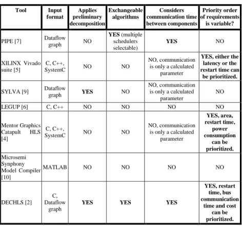
Table 1 summarizes some properties of several SLS tools.

Table 1

Overview of several SLS tools Tool Input

format

Applies preliminary decomposition

Exchangeable algorithms

Considers communication time between components

Priority order of requirements

is variable?

PIPE [7] Dataflow

graph NO

YES (multiple schedulers selectable)

YES NO

XILINX Vivado suite [5]

C, C++,

SystemC NO NO

NO, communication is only a calculated

parameter

YES, either the latency or the restart time can

be prioritized.

SYLVA [9] Dataflow

graph YES NO

parameter

NO

LEGUP [6] C, C++ NO NO NO NO

Mentor Graphics Catapult HLS [4]

C, C++,

SystemC NO NO

parameter

YES, area, restart time,

power consumption

can be prioritized.

Microsemi Synphony Model Compiler [10]

MATLAB NO NO NO NO

DECHLS [2]

C, Dataflow

graph

YES YES YES

YES, restart time, bus communication

time and cost can be prioritized.

(4)

2.1 Motivation of Choosing the SLS Tool DECHLS

Based on Table 1 the DECHLS can be considered as the most suitable tool for adaptation because it accepts dataflow graphs as its input, already includes a preliminary decomposition phase, its algorithms are accessible as well as variable and the priority order of the various requirements in its cost function is also variable. In the field of industrial control, the communication time between components can be similar of even longer than the execution time of some operations. Therefore, it is also required to consider the communication time which is not considered in the case of e.g. [6]. Modification is usually not allowed for commercial products such as [4, 5, 10]. Availability and potential modifiability of the DECHLS are the most important aspects to choose it. Also a motivation for choosing DECHLS is that it has been developed at the department of the authors.

The chosen SLS tool provides the results in form of XML files or dataflow graphs that suit the highest abstraction level. At the same time, the chosen application field (industrial process control) demands several special requirements also in the lower abstraction levels. Therefore, special adaptation and modification procedures are required in order to utilize the given results. Besides, the application field has its special widespread traditional, even standardized description and design methodology. In industrial process control, the component processors may be placed in large distances from each other. Therefore, the communication time between them can be significant and must not be neglected at adapting the SLS tool.

3 Adapting the DECHLS Tool

3.1 Industrial Process Control Systems as Special Cases of HMA

Modern industrial Distributed Process Control Systems (DCS) usually consist of many different intelligent modules. The modules of a DCS are usually connected by hierarchical and standardized bus systems. A DCS system performs a well- defined set of subfunctions distributed between several special programmable modules (often called programmable logic controllers, PLCs). Multiprocessing is a characteristic property of these systems, because the PLCs perform their functions concurrently with each other’s and repeatedly at prescribed cycle times.

A noticeable similarity exists between the DCSs and general HMA systems as shown in Fig. 1.

(5)

Component processor 1

Bus 1

Bus 2

Component processor 5 Component

processor 4

PLC PLC

HMI station

Actuator Sensor

Plant visualization

Central server Data logger

Central bus

Local bus 1 Local bus 2

Actuator Sensor Sensor

Figure 1

The general architecture of a HMA system (left) and that of a typical DCS (right)

The most problematic phase of a DCS’s design process is the task decomposition.

An additional special difficulty may arise, if the number of component processors is also prescribed. However, the DECHLS tool can be utilized in an adapted form to automate and optimize the design process of the DCS. The application strategy of the DECHLS-DCS adaptation is shown in Fig. 2.

Industrial control documentation (task description)

DECHLS-DCS

Implementation details:

 grouping of operations

 scheduling tasks

 applied IO and CPU modules

 connection of inputs and outputs

Evaluation data:

 Utilization of CPUs

 Utilization of busses

 Feasibility of the schedule

Modified industrial control documentation for more beneficial implementation

Figure 2

Strategy of adapting DECHLS for DCS design

3.2 Special Requirements of DCS

In an industrial process control project, many designer specialists usually must work together (e.g. architects, mechanical technologists, power engineers and control engineers) [11]. The complete documentation of the project must be understandable and unambiguous to all participants. Therefore, a traditional documentation form is already in use and it is standardized as IEC 61131 [11].

A new SLS approach to the DCS design must be adapted to this documentation form. This task description standard basically contains all inputs and outputs of the designed system and a formal description of the control algorithms to be

(6)

implemented. These control algorithms can also be designed by various graph- based methods. For example, [12] is based on a CP-graph model. Usually the control algorithm itself is already available as a dataflow-like graph. According to the [11] standard, the control algorithms are implemented by visual programming languages such as the Sequential Function Chart (SFC) or the Functional Block Diagram (FBD) [13]. Neither of these programming languages can be directly applied in the existing SLS tools. In order to adapt the DECHLS, a new dataflow graph model has been developed that is able to contain all information required by the standard description and it is also usable in DECHLS.

This new Functional Dataflow Graph (FDFG) can be summarized as follows:

} , , {V E F FDFG

(1) where V is the set of nodes, E is the set of directed edges and F is the set of subfunctions.

Every node in V represents an operation in the task description and a tuple of natural numbers is assigned to each node as:

} , {

, _i _i _i

i V v t m

v  

 (2)

where ti means the execution time of vi and mi is the required redundancy of vi. Every directed edge of the graph must have a source and a destination node and also must have a natural number assigned to it:

N c c e V v v v v e E

e_i _i  _a _b _a _b _i _i _i

 , { , }, , , , (3)

where ci is the number of data bits used in the communication between the two nodes belonging to the edge. The value of ci can also be 0, in this case there is no data communication, only timing dependency between vs and vd.

Set F consists of fi sets, each of them representing a subfunction. These fis are disjoint sets of nodes:

} ,..., , {f₁ f₂ f_n F

(4) where

F f V v v

f_i {..., _j,...}, _j , _i (5)

and

) , (

, _i _i _i

i F f T P

f  

 (6)

where Ti is a natural number that means the maximum possible execution time limit of fi. If this subfunction does not have a defined maximum execution time, then Ti should be 0. The Pi is a Boolean value; it is true if all parts of this subfunction must be allocated to the same processor.

(7)

3.3 Transforming the Task Description

As it is mentioned earlier, the FBD and SFC are not directly suitable as FDFG for DECHLS because of two problems. The first problem is with the order of the variable reads and writes. The second problem is that these graphs may have invalid execution orders or contain loops. These problems, however, can be solved by two simple algorithms as follows.

3.3.1 Handling Variable Reads and Writes

The PLC programs may contain variable reads and writes as elementary operations. These operations are used to access either actual data in temporary memory, or the physical inputs and outputs of the controller hardware. These read and write operations must be included into the resulting FDFG as part of the transformation process. The general rule of PLC software execution is that the program runs in a cycle. This must begin by reading all the input variables, then following by executing all the operations of the program. Finally, the modified variables should be written back. According to the IEC 61131-3 standard [11], variables should not be modified during a program unit’s execution. The reason of this is to prevent execution hazards. It also means that variable reads and writes must be handled separately. In this way, operations writing and then reading the same variable cannot be connected in the dataflow graph representation. This means that read operations never have inputs and they must be source nodes in the FDFG. Likewise, writes never have outputs and they must be destination nodes in the FDFG.

If more than one operation within a subfunction writes to the same variable, then only the latest write will be valid. Since the order of the writes is known already at the transformation stage, the invalid writes must be removed from the resulting FDFG. Therefore, the occurrence of such invalid writes can be considered as a possible error in the task description, and the transformation algorithm should warn the designer about this fact. Most commercial PLC development environments also perform this check and issue a warning. However, in case of alternative data paths and conditional execution of operations, the order of writes is determined by input data at runtime and cannot be determined during the transformation step. In these cases, the transformation algorithm should preserve all write operations.

3.3.2 Handling Prescribed Execution Sequence

An FDFG can have multiple valid and unambiguous execution orders. The rule to create an unambiguous execution order is that operations can only be executed if all their input data are present. In other words, after all the nodes having a directed path to this node are already executed. This rule allows for many different execution sequences considered valid ones. The output data yielded by any valid

(8)

execution sequence are the same. Therefore, both the designer, both the scheduling algorithm can freely choose each such valid sequence. It is easy to prove that an FDFG containing a cycle must not have any valid execution sequence.

An FBD program always prescribes the execution order of function blocks (i.e.

the elementary operations). After transforming the FBD into an FDFG, at least one of the valid execution orders in the FDFG must be the same as the prescribed execution order of the FBD.

If this prescribed execution sequence is also valid in the FDFG, then the graph needs not be modified further. However, if the prescribed execution sequence is not valid, then the FDFG must be modified into a form that makes the prescribed execution sequence also valid.

The following simple algorithm can be used to perform the aforementioned modification on the FDFG, as illustrated in Fig. 3:

1) Find an edge ei = (vs  vd), where vd precedes vs according to the execution order.

2) Create a new temporary variable.

3) Create a write operation for the new variable and create an edge leading from vs to this operation.

4) Create a read operation for the new variable and create an edge from vd to this operation.

5) Delete edge ei

6) Continue with step 1 until all the problematic edges have been tested.

V_s

2. V_d

1.

TMPei

TMP_ei X

2.

3.

4.

5.

Figure 3

Illustration of the steps needed to enforce the prescribed execution order

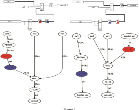
This algorithm can also be applied to solve the problem of cycles in the FBD. It is easy to prove that cycles in the FDFG will always contain at least one edge that will be found by the aforementioned algorithm. By performing the algorithm, this edge will be eliminated and the cycle will cease to exist. The effect of execution order on the resulting FDFG is illustrated in Fig. 4, where the FBD on the left and the FBD on the right differs only in the execution sequence order of the TO_IN and the TO_RE function blocks. The FDFG resulted from this valid execution order is seen on the left.

(9)

It can be observed that the execution sequence on the right means that the FDFG has two disjoint parts connected only by variables. Therefore, the TO_RE operation uses the previous output of the TO_IN operation that was saved from the previous cycle. It must be noted that this transformation also introduces one cycle of intentional signal delay between the affected blocks.

Fig. 5 illustrates the extended DECHLS flowchart adapted to DCS design.

Figure 4

Effect of execution order of the FBD on the FDFG

3.4 The Adaptation Algorithm

The proposed adaptation algorithm consists of the following phases:

 Transformation phase, that produces the FDFG from the standard task description formalism of the DCS (given in SFC or FBD languages). [14]

 Preliminary Functional Decomposition phase (PFD) prevents separating the user-defined logically coherent functions, in contrast to usual decomposition [15] algorithms.

 Multirate Function Scheduler phase (MFS) can enforce different cycle times (latency times) for some subfunctions in the FDFG [16].

(10)

 Extended Allocation phase (EA) that is also capable to handle additional replication constraints arising after the decomposition.

The aim of this step is to ensure safety-critical redundancy and availability, if any.

Node: operation Edge: data dependency Sets of nodes can have additional properties

Constraints and user requirements Description of the task for the system

SFC and FBD programming language implementation of the control system

Transformation to extended Dataflow

Graph

Preliminary decomposition (grouping operations)

Finding parallelization possibilities, ensuring required execution cycle time limits are met (Scheduling algorithm)

Allocating operations into tasks and to physical processing units (Allocation

algorithm)

List of applied CPU and IO modules Program lists of tasks (IL language) Connections of inputs and outputs

Execution time limits and cycle time limits for each function Description of control

algorithms

Definition of Inputs and Outputs

Execution time of elementary library

functions

Database of applicable CPU and IO modules

Definition of redundant or replicated subfunctions Previous Additional

Forming tasks based on:

execution time constraints minimizing communication time uniform CPU utilization

Elimination of race conditions Meeting execution time constraints by pipelining or multiplications if necessary

Definition of the functionally related operations (subfunctions)

Error if constraints are impossible to meet.

Utilization ratio of communication busses Utilization ratio

of CPU modules

Figure 5

Flowchart of the extended DECHLS tool adapted to DCS design

3.4.1 The Decomposition Phase

The main goal of the original preliminary decomposition in DECHLS is to reduce the number of elementary operations for the scheduler and allocation phases. In this way, the performance of those may be improved [2]. An additional benefit of the primary decomposition is that some special requirements can be taken into account with a higher priority. In case of DCS, the main goal of the decomposition is to distribute the workload uniformly along with also minimizing communication between segments. Segments will be treated as atomic in the scheduler. This means that operations assigned to the same segment will not be overlapping in time and cannot be allocated between multiple component

(11)

processors. Therefore, the decomposition can easily ensure that elementary operations of those subfunctions that must be allocated together due to the serviceability constraint (Pi = true) should never overlap in time. Each of such elementary operation will form a separate segment, independently of the other segments.

There can be more decomposition algorithms used in DECHLS. The spectral clustering based algorithm has proved to be the most suitable for industrial control system tasks because it is capable to a simpler parameterization [14, 2].

3.4.2 The Scheduling Phase

The scheduler algorithm used in DECHLS is a modified force directed one [7].

The scheduler can be simplified because pipeline execution in DCS systems is usually not allowed.

In this case, the scheduler only needs to determine the starting time of the segments created already in the decomposition step. This starting time of most segments can range up to the maximum cycle time (the latency time, L), which is an input parameter to the scheduler. A minimum latency (Lmin) can also be determined based on the shortest execution path in the FDFG. The scheduler cannot find a valid solution when L<Lmin, therefore it must stop in this case. Such minimum latencies also exist for each subfunction (subgraph) of the FDFG.

Some functions (segments) must be completed faster than L, because their prescribed cycle time is Ti<L. The force directed algorithm should be modified to take into account the Ti of each subfunction by implementing a multi-rate scheduler as in [16].

The multi-rate scheduler has different queues for different operation groups as seen in Fig. 6. Operations belonging to subfunctions without a defined execution time limit will be scheduled in the general queue. Subfunctions, having longer or equal execution time limits than the given latency, are also scheduled in this general queue because their execution time limits will be trivially met.

Subfunctions having a smaller time limit than L must be handled in different queues. The queue of function fi with time limit Ti will have a multi-rate latency of Li, where

i

i k

L  L



 





i

i T

k L

(7) All the separate queues will have the same force function, and operations potentially overlapping in any queues will increase the force. Because of this, the scheduler will attempt to prohibit overlapping operations as long as possible in order to reduce the required number of processors. There is one more important task of the scheduler. If any subfunctions’ minimum latency (Lmin,i) defined by its

(12)

FDFG is smaller than its specified Ti, then the scheduler must report an error and stop. In this case, the execution time constraints are too strict and cannot be met by this algorithm.

v1

General queue:

v2 v3 v6 v7

L

fi queue: v4 v5 v4 v5 v4 v5

Li Li

Li

Ti

Figure 6 Multi-rate scheduler

3.4.3 The Allocation Phase

The allocation phase is the simplest among the modifications. It should be able to allocate mi copies of every operation. These multiple copies must be allocated into different processors, irrespective of their timings. This can be done even before the actual allocation phase as a previous step, or by slightly modifying an existing allocation algorithm. In case of the graph-coloring based algorithm in DECHLS, this modification can be done in the following way.

The existing allocation algorithm builds a conflict graph, based on the scheduled dataflow graph. The nodes of this conflict graph represent the nodes of the scheduled dataflow graph, but the edges in the conflict graph represent the time overlapping between nodes. If two operations are overlapping in time, they cannot be executed by the same component processor. In this sense, the allocation basically means the coloring of the conflict graph, by the least amount of colors.

Thus, any two adjacent nodes are colored differently.

In case of DCS, the redundancy criteria may require the replication of certain nodes. Those nodes are already replicated before scheduling and they will appear as two separate nodes in the scheduled dataflow graph. Since multiple copies of the same logical node are scheduled independently, it may happen that they are not overlapping. However, they are not allowed to be allocated into the same processing unit because their multiplication would not result a real redundancy.

Such a scenario is seen in Fig. 7, where nodes 5, 6 and 7 are replicated (5’, 6’ and 7’). The scheduler placed some of the replicated nodes into different time slots for minimizing the resource usage. In this way, only 3 processors will be required.

(13)

1

OUT 3

4

5 6

7

9

IN1 IN2 IN3 IN4

Time step 1

Time step 2

Time step 3

Time step 4 6’

7’

5’

2

8

Figure 7

An example for a scheduled dataflow graph with replicated nodes

In order to solve the problem, additional edges are needed in the conflict graph between redundant copies of the same node. In Fig. 8 these edges are marked as double lines for easy identification. Otherwise in the remaining steps of the graph coloring algorithm, these additional edges are treated the same as regular edges.

This way, the redundancy can be safely handled, by the allocation algorithm.

7

6

2

3 1

8

4 6’

7’

9 5’

5

Figure 8

A conflict graph with the additional edges and a possible coloring

(14)

4 Benchmark Results

The chosen benchmark application is an existing DCS that was programmed in the FBD language by using the ABB Freelance development environment [17]. The benchmark consists of 29 program blocks. Each of the program blocks are logically coherent functions. Some blocks are scheduled to operate with 1000 ms, while others with 500 ms cycle times. The program blocks are distributed between two separate ABB AC800F3 PLCs. There are two special functions that redundantly implement the same safety critical function (burner control). These two tasks must never be allocated to the same PLC for safety reasons. This is the main reason why two PLCs were needed in this implementation.

The first step is the transformation of the existing FBD task description into FDFG form. Only an essential part of the original description (one subfunction) and the resulting FDFG is illustrated in Fig. 9 and Fig. 10.

The FDFG was then given to the preliminary decomposition phase and the algorithm divided it into 97 subfunctions instead of the original 29. For example, the #27 subfunction was divided into 6 parts as illustrated in Fig. 11. Increasing the number of subfunctions provides more freedom in the later phases, namely the scheduling and the allocation.

The purpose of Figs. 9, 10 and 11 is only to illustrate the structures of the original and the transformed graphs, the text fields in the blocks are not important in this sense.

After the decomposition, the scheduler and allocation phases of the experimental DECHLS-DCS tool have determined the required number of PLCs. The average utilization of PLCs as well as the average communication bus utilization at several different cycle times were also computed and these are shown in Fig. 12.

The cycle times indicated in the Fig. 12 are the longest ones in each case, some functions have shorter cycle times. The reason of this is the fixed 500 ms cycle time of the critical functions in the original implementation. For the rest of the functions, there are no cycle time prescriptions. If the actual cycle time is shorter than the prescribed one, the whole system runs at the actual cycle time. If the actual cycle time is longer, then the critical functions must still run at least as fast as the prescribed cycle time. The diagram has markers at specific cycle time values to show where practical solutions are obtained. Between 400 ms and 450 ms there are many markers, because the tool was restarted many times in this interval in order to find the shortest possible cycle time allowing the task to be solved by only 2 processors.

(15)

Figure 9

FBD form of subfunction #27 in the benchmark

Figure 10

FDFG form of subfunction #27 in the benchmark

(16)

Figure 11

The 6 new subfunctions resulted from subfunction #27

0 1 2 3 4 5 6 7 8 9 10 11

0 100 200 300 400 500 600 700 800 900 1000

Cycle time [ms]

Number of CPU modules [db]

0%

10%

20%

30%

40%

50%

60%

70%

80%

90%

100%

Utilization [%]

Number of PLC CPU modules Utilization of CPU modules Utilization of communication busses

Figure 12

The resulted number of PLCs and their utilization levels at different cycle times

Fig. 12 shows in the left axis that only 2 PLCs are required at 450 ms cycle time (blue line). In this case, the average utilization (purple line) is only about 80%, as seen on the right axis. All functions are still able to run at this speed. Less than 2 PLCs are never enough to solve the task, because of the redundancy constraint. It can be observed that prescribing 1000 ms cycle time was not necessary in the existing implementation.

The DECHLS-DCS also shows that the average utilization of CPUs and communication busses in the existing system were only around 37% and 11%.

The official ABB Freelance development tool cannot deliver such estimations without completely building the system, followed by downloading, running and profiling the whole software.

(17)

Summarizing above simulation results:

 A 450 ms cycle time could be achieved safely by utilizing the same number of CPUs

 79% CPU utilization was achieved instead of 37%

 22% communication bus utilization was achieved instead of 11%

Conclusions

This paper has illustrated how an SLS tool (DECHLS) can be adapted, modified and utilized in designing a specific form of HMA (an industrial process control system). For this proper adaptation, DECHLS have been modified in order to be capable to handle the application-specific standardized task input graph descriptions (SFC or FBD). A converting algorithm has been presented for this extension. The additional necessary extensions for adaptation have been also presented in the paper: a special decomposition algorithm, a multirate function scheduler algorithm, an extended allocation algorithm handling safety-critical redundancy. By these modifications and extensions, DECHLS became a capable tool for providing various resulting designs to compare and evaluate them already on the SLS level without any lower level implementations.

The benchmark presented in the paper illustrates on comparing with existing solutions that the preliminary decomposition in DECHLS increased the number of subfunctions. Hereby, more freedom remains for the scheduling and allocation phases. It can also be observed that a proper systematic scheduling could lead to higher processor utilization even at high communication times between processors.

Consequently, such an adaptation of the DECHLS tool, helps to compare and evaluate various resulting HMAs exclusively on the SLS level, without implementing the whole system.

References

[1] Gy. Rácz, P.Arató, „A System-Level Synthesis Approach to Industrial Process Control Design”, 23^rd IEEE International Conference on Intelligent Engineering Systems, Gödöllő, Hungary, 2019

[2] Rácz, Gy.; Arató, P. "A decomposition-based system level synthesis method for heterogeneous multiprocessor architectures," 2017 30^th IEEE International System-on-Chip Conference (SOCC), Munich, Germany, 2017, pp. 381-386

[3] W. Meeus, K. Van Beeck, T. Goedemé, J. Meel, D. Stroobandt, “An overview of today’s high-level synthesis tools”, Design Automation for Embedded Systems, 16(4), 31-51, 2012

[4] Mentor Graphics Catapult C software manual:

https://www.mentor.com/hls-lp/catapult-high-level-synthesis/

(18)

[5] Xilinx Vivado design Suite Manual:

https://www.xilinx.com/products/design-tools/vivado.html

[6] A. Canis, J. Choi, B. Fort, B. Syrowik, R. L. Lian, Y. T. Chen, H. Hsiao, J.

Goeders, S. Brown, J. H. Anderson, "LegUp High-Level Synthesis,"

chapter in FPGAs for Software Engineers, Springer, 2016

[7] P. Arató, T. Visegrády, I. Jankovits, “High Level Synthesis of Pipelined Datapaths“, John Wiley & Sons, New York, ISBN: 0 471495582 4, 2001 [8] N. Govil, S. R. Chowdhury, “GMA: a high speed metaheuristic algorithmic

approach to hardware software partitioning for Low-cost SoCs”, 2015 International Symposium on Rapid System Prototyping (RSP), Amsterdam, 2015

[9] L. Shuo, “System-Level Architectural Hardware Synthesis for Digital Signal Processing Sub-Systems.” PhD thesis, Stockholm, 2015

[10] Microsemi Synphony Model Compiler User Guide:

https://www.microsemi.com/product-directory/dev-tools/4899- synphony#documents

[11] IEC, IEC 61131 en:2003, Programmable Controllers

[12] K. M. Hangos, F. Friedler, J. B. Varga, L. T. Fan, “A graph-theoretic approach to integrated process and control system synthesis”, IFAC Proceedings Volumes, 27(7), 1994, 61-66

[13] IEC, IEC 61131-3 en:2003, Programmable Controllers - Part 3:

Programming languages, 2018

[14] Gy. Rácz, P. Arató, “Adapting the system level synthesis methodology to industrial control design”, Proceedings of the Workshop on the Advances of Information Technology: WAIT 2018, Budapest, 2018, 131-136

[15] P. Arató, D. Drexler, Gy. Rácz, “Analyzing the Effect of Decomposition Algorithms on the Heterogeneous Multiprocessing Architectures in System Level Synthesis” Scientific Buletin of Politechnica University of Timisoara Transactions on Automatic Control and Computer Science, 60(74) 39-46, 2015

[16] X. Y. Zhu, M. Geilen, T. Basten and S. Stuijk, "Static Rate-Optimal Scheduling of Multirate DSP Algorithms via Retiming and Unfolding,"

2012 IEEE 18^th Real Time and Embedded Technology and Applications Symposium, Beijing, 2012, 109-118

[17] ABB Freelance Engineering, https://new.abb.com/control- systems/essential-automation/freelance/engineering