CHAPTER TWO KINETIC MOLECULAR THEORY OF GASES

CHAPTER T W O

KINETIC

MOLECULAR THEORY OF GASES

2-1 Introduction

The treatment of ideal and nonideal gases in Chapter 1 was carried out largely from a phenomenological point of view. Behavior was described in terms of the macroscopic variables Ρ, V, and Γ, although some molecular interpretation was included in the discussion of the a and b parameters of the van der Waals equation (Section 1-9) and in the Special Topics section. We take up here the detailed model of a gas, that is, the kinetic molecular theory of gases. In this model, a gas is considered to be made up of individual molecules, each having kinetic energy in the form of a random motion. The pressure and the temperature of a gas are treated as manifestations of this kinetic energy. In its simplest form, kinetic theory assumes that the molecules experience no mutual attractions.

The elementary picture is the familiar one of a molecule having an average velocity u and bouncing back and forth between opposite walls of a cubical container. With each wall collision a change in momentum 2mu occurs, where m is the mass of a molecule. If the side of the container is /, the frequency of such collisions is u/2l, and the momentum change per second imparted to the wall, that is, the force on it, is mu²/l. The pressure, or force per unit area, becomes mu²/l³ or mu²/\. The quantity u refers to the velocity component in some one direction, and the total velocity squared, c², is c² = u² + v² + w², where ν and w are the components in the other two directions; on the average these components should be equal, and so we conclude that u² = c²/3, and obtain the final equation

Pv = \mc², (2-1)

where ν denotes the volume per molecule. Per mole, this becomes

PV = \Mc², (2-2)

where Μ is the molecular weight of the gas.

One now takes note that the simple picture corresponds, for real gases, to the 39

limiting condition of zero pressure, for which the phenomenological law is the ideal gas equation

PV = RT (2-3) and the relationship which is intuitively expected to exist between kinetic energy

and temperature is simply

RT == | M c² = §(kinetic energy), (2-4) the molar kinetic energy being \Mc². Alternatively, one writes

* = I? <

-

>

or

McT

C2 =

i^L

where k is the gas constant per molecule, called the Boltzmann constant, as noted in Section 1-7.

This treatment is unsatisfactory at some points. Clearly, it is unrealistic to take all molecules as having the same velocity. Even occasional intermolecular collisions must eventually bring about a distribution of velocities, and since we are describing a theory for time-invariant or equilibrium properties of a gas, we should be dealing with velocity distributions. The quantity c² must then really be some kind of average quantity. The argument that one should use \c² for the velocity component squared in some one direction is plausible but is not a proof. The sections that follow take up a more elaborate but more satisfying way of obtaining not only the above results, but much additional information as well.

There remain a number of important properties of a gas which cannot be explained unless a finite molecular size is specifically assumed. The model at this point becomes one of molecules that act as hard spheres. By " h a r d " we mean that they behave like spheres of definite radius r and that their collisions are elastic so that kinetic energy as well as momentum is conserved. Beyond this lie more advanced treatments which allow for the presence of attractive as well as of repulsive forces between molecules. Some aspects of these will be taken up in the Special Topics section.

The immediate task, however, is the treatment of velocity distributions. Here the central assumption will be that of the Boltzmann principle. As was stated in Section 1-7, according to the Boltzmann principle the probability of a molecule having an energy e is given by

p(^€) = (constant) e~^^kT. (2-7)

This principle was adduced as a generalization of the barometric equation; it can, however, be reached in other ways, one of which is given in the next section.

2-2 The Boltzmann Distribution Law

The Maxwell-Boltzmann principle (often referred to as the Boltzmann principle) is so central to all of the statistical aspects of physical chemistry that it merits a

2-2 THE BOLTZMANN DISTRIBUTION LAW 41 TABLE 2-1. Ways of Distributing Molecules

between States'¹

System

N u m b e r in given state6

System «i = 1 *² = 3 €³ = 5

1 5 5 0

2 6 3 1

3 7 1 2

a Assuming ten molecules and total system energy of 20 units.

b Energy in arbitrary units.

more general derivation than that of Section 1-7. We want to consider a system that is isolated, so that its total energy Ε is constant and the total number of molecules Ν is also constant. The molecules making up this system can have various quantized energy states; let them be called c¹, e², €³, and so on.

There will be many ways in which the Ν molecules could be assigned specific energies so as to give the same total energy E. For example, let Ε be 20 units of energy and Ν be ten molecules, and suppose that there are three possible states of one, three, and five units of energy. Possible distributions are given in Table 2-1.

In this case there are three different ways of satisfying the two requirements of fixed Ν and fixed E.

The statistical weight that we want is obtained as follows. If we were just putting Ν molecules in as many boxes, their permutations would be N\. However, we consider only molecules in different energy states as distinguishable. That is, the Ν^τ molecules in the €¹ box are taken to be indistinguishable, as are the N² molecules in the e² box, and so on. We must then divide out the permutations that should not be present. Thus in the case of system 2, there are 6! ways of permuting the molecules in the *¹ box, 3! ways for the e² box, and 1! or one way for the c³ box.

The distinguishable permutations, which give the desired statistical weight, are thus 10!/(6!)(3!)(1!) = 840.

The general statements of the preceding conditions are then

Ν = £ Ν⁴• = constant, (2-8)

Ε = £ Ni€^t = constant, (2-9)

W AM

where N^{ denotes the number of molecules in the zth state of energy e^e and W is the statistical weight or probability of the particular distribution. To repeat, the denominator of Eq. (2-10) serves to take out those permutations that do not count because of the indistinguishability of molecules in the same energy state.

One further point completes the basic picture. If Ν is a very large number, for example, Avogadro's number, it turns out that W will peak very sharply at some one distribution. That is, there will be some set of N^l9N², and so on values giving the largest W, and relatively small departures from this proportion will cause W to drop sharply. This largest W is called W^m2LX. Thus the set of requirements of

Eqs. (2-8)-(2-10) acts to define a most probable distribution and one which is assumed, in the case of a large number of molecules, to be the distribution.

The preceding conditions and assumptions are in fact sufficient to give the immediate precursor to the Boltzmann distribution law, namely the conclusion that

p(^€) = (constant) e~^&\ (2-11)

where p(e) is the probability that the molecule has energy e . The constant β will be identified with I/kT in Section 2-6, when a consequence of Eq. (2-11) is com­

pared with the ideal gas law.

First, we can obtain Eq. (2-11) as follows. Since we are considering a system at equilibrium, the distribution will be one for which W is at a maximum—that is, we expect the equilibrium distribution to be the one that is the most probable. We now imagine that a small redistribution δ of molecules takes place, subject to the restriction that neither T V nor the total energy of the system changes,

i

Σ

*δ^

i

Since Wis at a maximum, it also follows that hWmust be zero. It is convenient at this point to take the logarithm of Eq. (2-10):

In W = In Nl - £ l n t f , !

i

and write as the condition

8(ln W) = 0 = £ 8(ln N^{\) (2-14)

i

since δ(1η Ν Γ) = 0. We are dealing with very large numbers and it is permissible to replace factorials by Stirling's approximation,

In xl = χ In χ — χ. (2-15) Equation (2-14) becomes

0 = £ 8 ( t f , In

i

= Σ

+ Ο"

δ*, -

i ¹

Σ (In N^t) 8Ν^{ = 0. (2-16)

i

Equations (2-12)-(2-14) impose three different conditions on the SN's and are to be obeyed even though the system makes small, arbitrary fluctuations. A way of handling such a situation is Lagrange's method of undetermined multipliers [see, for example, Blinder (1969)]. We add the three conditions, but in some ratio which is to be determined; that is, we write

X (a + 06, + In N^t) 8N^{ = 0, (2-17)

i

where Eqs. (2-12) and (2-13) have been multiplied by the undetermined coefficients OL and j3, respectively.

2-2 THE BOLTZMANN DISTRIBUTION LAW 43 Lagrange's m e t h o d is very useful for finding what is k n o w n as a conditional m a x i m u m (or m i n i m u m ) , that is, for finding a m a x i m u m (or m i n i m u m ) in a function subject to the constraint that s o m e other relationship also holds. In the present case, w e seek a m a x i m u m in In W, but subject to the constraints of Eqs. (2-8) and (2-9), that is, t o the requirement that the total n u m b e r of molecules and their total energy be constant.

A s a simple illustration, suppose that o n e wishes t o maximize the area o f a rectangle subject to the constraint that its perimeter be constant. W e thus have xy = si and 2x + 2y = s⁹ where χ and y are the sides and s/ and s the area and perimeter, respectively. B y the variation m e t h o d , w e write

y 8x + χ 8y = 0, 2 8x + 2 δ ; = 0, a n d , introducing the undetermined multiplier, a,

(y8x + x8y) + a(28x + 2 8 ; ) = 0, or

(y + 2a) 8x + (x + 2a) 8y = 0.

Again, if the variations χ and y are t o be arbitrary, each term separately must be zero, and w e find y + 2a = 0 and χ + 2α = 0, w h e n c e χ = y = —2α. T h e figure o f m a x i m u m area for a given perimeter is thus a square.

In the case o f the rectangle, the s a m e answer c a n b e found by ordinary calculus. W e eliminate y between the t w o equations, to get

O n setting the derivative ds/Jdx = 0, w e find 2x = s/2, w h e n c e 2y = s/2 and thus χ = y.

Equation (2-17) can be written out in detail as a sum of terms in δΛ^ , 8N², 8N^S , and so on:

(α + β^€ι + In N^x) SN^X + (a + βε² + In N²) 8N²

+ (oc + β€³ + In NJ 8N^Z + - = 0. (2-18) Now, if there were only two states, say e^x and €², Eqs. (2-8) and (2-9) would abso­

lutely fix the distribution (for example, system 1 of Table 2-1). With three states the most probable population of €³ could be varied, but given 8N^B, this would then determine δΛ^ and 8N². With a larger number of states, δ #³, 8N^A, and so on could be chosen arbitrarily, and this would then fix δΛ^ and δΛ^². If we elect to choose values for α and β such that the terms of Eq. (2-18) in δΛ^ and 8N² are zero, which can be done since α and β are adjustable constants, then the equation reduces to the requirement that the sum of all the terms in δΛ^ , δΛΓ⁴ , and so on must be zero. Since the variations 8N^S, δ Ν⁴, and so on are arbitrary, the only way for this requirement to be generally true is for each term separately to be zero. The general condition is therefore

OL + β^{€ ί} + In N^t = 0 (2-19) or

N^€ = e-^ae~^B€i = (constant) e~^0ei, (2-20) which is Eq. (2-11).

This result, namely that the most probable number of molecules in a state of energy €^t is proportional to e~^0€i, may seem startling in that it is obtained on so general a basis. To repeat, it is a consequence of the restrictions of Eqs. (2-12)- (2-14) plus the assumption that molecules will find that energy distribution having the greatest statistical weight as given by the permutation formula of Eq. (2-10).

2-3 The Distribution of Molecular Velocities

We start by applying the Maxwell-Boltzmann distribution equation (2-7) to the case of a one-dimensional gas, that is, to a system of molecules having only kinetic energy due to motion along one direction in space, say the χ direction. The Boltzmann equation then gives

( ^{— (}

⁰

where w is the velocity in the χ direction (and could be either positive or negative), and € = J raw². The more quantitative way of stating Eq. (2-21) is to say that it gives the fraction of molecules dN(u)/N⁰ (where N⁰ is the total number of molecules, taken here to be Avogadro's number) having velocities between u and w + du,

dN(u)

The proportionality constant A can be evaluated by the requirement that the sum of probabilities for all possible velocities must be unity:

JT-'-"CM-sr)K <w

The integral of Eq. (2-23) can be put in a standard form, that is,

f [ e x p ( - a²*²) ] dx = ^ - , (2-24) where in the present case a = (m/lkT)¹^. Because the distribution must be sym­

metric with respect to plus and minus directions, we have

i:N-w)]*=

/:H-^)]"»-m"

The constant A, called the normalization constant, is thus (m/lnkT)¹/² and Eq.

(2-22) becomes

dN(u) ι m x¹/² r / raw² \i , „ „

n ^

( - w ) H-2*r)r

-

-

The plot of Eq. (2-25), that is, of (l/N⁰) dN(u)/du versus w, is shown in Fig. 2-1 for the case of a gas of molecular weight 28, such as nitrogen, at 25°C and 1025°C.

The coefficient of w² can be written M/2RT and is thus equal to 28/(2)(8.314 χ 10⁷) (298.1) = 5.649 χ 10"^{1 0} at 25°C and 1.297 χ 10"^{1 0} at 1025°C, with w in centi­

meters per second. The coefficient A can likewise be written (M/lnRT)¹/² and has the values 1.34 χ 1 0^{- 5} and 0.644 χ 1 0^{- 5} sec c m^{- 1} at the two temperatures, respectively. Note that the distribution is symmetric and that the most probable velocity is zero. This latter statement is true because there are equal chances for a molecule to gain a velocity increment in either the positive or the negative direction. Finally, the spread of the distribution, as measured, for example, by the width at half-maximum, increases with increasing temperature.

The case of a two-dimensional gas follows in a straightforward manner. We now allow velocities along the χ and y directions, given by w and v. The net velocity c

2-3 THE DISTRIBUTION OF MOLECULAR VELOCITIES 45

- 1.5 x 10 5

\ 25 °C

V- l.o χ io~

-0.5 x 10

\s.

1 1

V \ 1025°C

1 ^ ^ _ J

-10 0 10

u χ 10⁴, cm sec ¹

F I G . 2 - 1 . Molecular velocity distribution in one dimension for N²

of a molecule having components u and υ is c² = u² + v² and the Boltzmann equation is

dN(u,v) _ ^A \ _ i m(u² + v²) No A]exp\

2kT j

J

(2-26)

(2-27) where dN(u, v)/N⁰ is now the fraction of molecules having velocity components between u and u + du and ν and ν + dv. Equation (2-27) factors into two integrals, each analogous to that of Eq. (2-23), with the result that on carrying out the normalization procedure, one finds that A = m/2nkT, and the complete distri­

bution equation becomes dN(u⁹ v)

No = 2 5 r |^{e x p}[ - ^m(u

2

+

2kf

•11

The distribution function of Eq. (2-28) now requires a three-dimensional plot for its display, as illustrated in Fig. 2-2. Again the maximum is at u and ν equal to zero, and, of course, it is symmetric with respect to positive and negative velocities.

It is ordinarily of more interest to deal with the net velocity c than with the separate components. That is, although the u and ν velocity components represent independent ways in which the molecule can have kinetic energy, it is the net velocity of the molecule and its total kinetic energy mc²/2 that are needed for most applications. Now the sum of all the possible ways in which the net velocity can

(\IN⁰)dN(u)ldu

increase from c to c + dc, that is, by adding increments du and dv to various combinations of u and v, is given by the area of the annulus shown in Fig. 2-2.

V

[-dc

du\ J

F I G . 2 - 3 .

This argument is illustrated in more detail in Fig. 2-3. The effect is that du dv can be replaced by 27rc dc, so that the distribution law becomes

dN(c) m

r /

\ i , _

^ = ΐτί

(-w)F

-

-

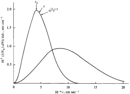
The two-dimensional distribution law for c, Eq. (2-29), can now be plotted on an ordinary graph, since only the net velocity is involved; also we have lost the information as to whether c is positive or negative and plot only its magnitude.

Some sample graphs, again for a gas of molecular weight 28, are shown in Fig. 2-4.

Notice that there is now a nonzero most probable velocity, in contrast to the situation in Fig. 2-2. The reason is that, while the probability of individual velocity components u and ν decreases with their increasing values, the number of ways in which a given velocity magnitude c can be made up of the u and ν components

F I G . 2 - 2 . Molecular velocity distribution for a gas in two dimensions.

2-3 THE DISTRIBUTION OF MOLECULAR VELOCITIES 47

0 5 10 15 20 10 ⁴ c, cm sec _ I

F I G . 2-4. Molecular velocity distribution for N² in two dimensions.

increases in proportion to c. For a while the latter effect overrides the former.

Notice also that the most probable c value increases with increasing temperature and that the half-width increases with increasing temperature.

The extension to three dimensions follows the same series of steps. The basic distribution law is

dN(u, v,w) A r m(u² + v² + w²) τ ) , , , ^{/ f %} - ^m

— = ^A

l

L i k f — J !

^

·

where w is the added velocity component in the ζ direction. This again can be factored into three integrals, so that the normalization constant becomes the cube of that for the one-dimensional gas, to give

N⁰ - ( - W ) Η 2kf \\dudvd^W. (2-31) Again the chief interest is in the net velocity, now given by c² = u² + v² + w², and the number of ways in which a velocity increment dc can be obtained is related to the separate increments by

477-c2 dc = du dv dw.

The distribution law in net velocity c is then

Example. Calculate p(c) for 02 at 2 5° C a n d c = 1 χ l O ' c m s e c "1. T h e ratio m/2kT — M/2RT= ( 3 1 . 9 9 9 ) / ( 2 ) ( 8 . 3 1 4 3 3 x 1 07) ( 2 9 8 . 1 5 ) = 6 . 4 5 4 2 x 1 0 "1 0 and mc2/2kT = 6 . 4 5 4 2 , s o that Qxp(-mc2/2kT) = 1 . 5 7 3 9 Χ 1 0 "8. Substitution into Eq. ( 2 - 3 2 ) gives

p(c) = 4 τ τ ( 6 . 4 5 4 2 Χ 1 0 -1 0/ τ γ )8 / 2/ ( 1 . 5 7 3 9 Χ 1 0 -8) ( 1 Χ Ι Ο5)2 = 5 . 8 2 4 χ Ι Ο "7.

In SI units, M/2RT = ( 0 . 0 3 1 9 9 9 ) / ( 2 ) ( 8 . 3 1 4 3 3 ) ( 2 9 8 . 1 5 ) = 6 . 4 5 4 2 χ 1 0 " · , mc2/2kT = 6 . 4 5 4 2 (or the same, as it must be since the exponential is dimensionless and therefore cannot depend o n the choice of system of units). T h e n

p(c) = 4 π ( 6 . 4 5 4 2 χ 1 0"βΑ 08 / 2( 1 . 5 7 3 9 χ 1 0 "8) ( 1 χ 1 08)2 = 5 . 8 2 4 χ 1 0 "6.

N o t e that p(c) is a hundredfold larger in the SI calculation. This is because the velocity interval dc is 1 0 0 times larger w h e n c is in m s e c "1 than w h e n it is in c m sec" *.

Equation (2-32) is plotted in Fig. 2-5 and looks much like the one for a two- dimensional gas. The maximum or position of most probable velocity has moved outward, however. This most probable velocity c^p may be evaluated analytically if dp(c)/dc is set equal to zero. On doing this, one obtains from Eq. (2-32) the con­

dition

- w H - w)]<w>+ H- #)] α*>=ο

or

lie Τ

cf = ^ ~ - (2-33) As a final comment on the general character of these distribution laws, we note

that the probability of a given velocity rapidly decreases with increasing c owing to the exponential term. There is, however, always a finite probability for any given velocity, no matter how large. For example, the fraction of molecules per unit velocity increment having a velocity of 5c^p is only about 1 0^{- 1 0} of that having

FIG. 2-5. Three-dimensional velocity distribution for N2.

2-4 AVERAGE QUANTITIES FROM THE DISTRIBUTION LAWS 49 velocity c^p itself. Such a number, although small, can be quite significant when chemical reaction rates are being treated.

2-4 Average Quantities from the Distribution Laws

It is a common experience to take the average of some property for a collection of objects. For example, the average value of a coin in a bag of mixed coins would be obtained by dividing the total value by the number of coins. In more detail, the operation is one of dividing two sums:

° = TW-

-

That is, the product of the value s^{ of the ith type of coin times the number N^{ of such coins is summed over all types and is then divided by Σ N^{, the total number of coins. The average of any property could be obtained in this way; if s denotes the mass of a given type of coin, then s would now be the average mass of a coin, and so on.

If there are a very large number of objects with many gradations of the property s, then these summations can be approximated by an integration procedure. The principal change is that N^t is now replaced by a probability or distribution function N(s), where dN(s) gives the chance of finding objects with s lying between s and s + ds:

its dm

r

The integral J^° dN(s) simply represents the sum of all objects and must therefore equal N⁰ , their total number.

We can apply Eq. (2-35) to obtain two important types of average velocity for the three-dimensional case. The first is simply the average velocity c given by

c = ± - f cdN(c) or

The integral may be evaluated as follows. We let χ = mc²/2kT, and so obtain

/ m \3/2 / IrT \2 Λ0 0

The integral is now a standard one known as a gamma function¹ and its value is

+ Integrals of the type / " j c^{n _ 1} e~^x dx occur frequently in physical chemistry; this integral is called the g a m m a function Γ(η). Standard tables of Γ(η) are available for 0 < η < 1 and 1 < n<2;

s o m e important values are Γ(1/2) = and Γ(1) = 1. Also, a very useful relationship is Γ(η+\)

= ηΓ(ή) for η a positive integer.

- ^ - ) = 1 . 1 2 8 c^p [Eq.(2-38)], 3kT \V2

average c

root mean square {c²)¹'² = ( ^ — ) = 1.225c^p [Eq. (2-40)].

These three velocities are located on one of the distributions of Fig. 2-5 so as to show their relative positions.

2-5 Some Applications of Simple Kinetic Molecular Theory.

Collision Frequency on a Plane Surface and Graham's Law

An important quantity given by simple kinetic molecular theory is. the frequency with which molecules hit a plane surface. This frequency is, for example, central to the kinetic treatment of adsorption-desorption processes or, more generally, to those of evaporation and condensation.

The relationship can be derived fairly simply as follows. Since all directions in space should be equivalent, the result should be independent of direction; we can therefore assume that the molecules impinging on a plane surface are doing so from the χ direction, so that only their velocity components in that direction need just unity. The resulting expression for c is thus

c = (2-38) The second average is that of c²; this is given by

?

-Mwfj; M--Sr)]«**- ™

When we let χ = mc²/2kT the integral reduces to one of the form x^zl²e~^x dx, again a gamma function, and one whose value is | ViF [see the footnote following Eq. (2-37)]. On working through the algebra, we find

m

or, alternatively, the average molar kinetic energy Ε is then

Ε = \RT. (2-41) Note that the right-hand sides of Eqs. (2-6) and (2-40) are identical. Thus the

average velocity referred to in the mtroductory section is really the square root of the average of velocities squared, ( c²)^{1 / 2}, or the root mean square velocity. See also Section 2-6.

In conclusion to this section, the three characteristic velocities for a gas in three dimensions are

/ 2kT x1/2

most probable c^v = (-Jjj—) [Eq. (2-33)], SkT \!/2

2-5 SURFACE COLLISION FREQUENCY; GRAHAM'S LAWS 51 be considered. The distribution law for such χ components is given by Eq. (2-25):

where η and n⁰ denote numbers of molecules per unit volume, n⁰ being the total concentration; dn(u)/n⁰ is again the fraction of molecules having velocity between u and u + du.

F I G . 2-6. Volumes swept out in unit time by molecular velocity groups u^x and u².

As illustrated in Fig. 2-6, if we consider a particular group of molecules of velocity component u^x, the ones that will reach the surface in the next second will be those within the distance x¹, where x¹ = u^x. Per unit area of surface, the total number of molecules of this velocity group reaching the surface per second will then be n(u^)u^x (since u^x times the unit area gives the volume containing the success­

ful molecules of that velocity group). For some other group of, say, lower velocity u² the number of that group reaching the surface per second will be n(w²)w² · In effect, then, we need to weight the distribution equation by u to get dZ(u)⁹ the number of molecules per unit volume reaching the wall whose velocity com­

ponent lies between u and u + du:

We obtain Z, the total surface collision frequency per unit area, by integrating over all acceptable values of w, namely from zero to plus infinity, where a plus velocity is one toward the surface. On carrying out this integration, we obtain

(the subscript to the concentration η is no longer needed).

Equation (2-43) can be phrased in some alternative ways. On referring to Eq.

(2-38) for the average velocity c, we see that

(2-42)

(2-43)

Ζ = Inc. (2-44)

Alternatively, the kinetic molecular theory at this level of sophistication implies ideal gas behavior, and since the concentration η is then equal to P/kT, we have

/ 1 χ¹/² / I x¹/²

z

= ' f c y -"^SBSF) • »">

Finally, the mass collision frequency Z^m follows if Ζ is multiplied by the mass per molecule:

kT \^²

where ρ is the density.

The preceding discussion provides a theoretical basis for understanding a con­

clusion reached in 1829, known as Graham's law. Graham studied the rate of effusion of gases, that is, the rate of escape of gas through a small hole or orifice.

He found that for a given temperature and pressure difference, the rate of effusion of a gas is inversely proportional to the square root of its density. For two different gases, then, we have

^ = ( ^ f * (2-47) where η denotes the number of moles escaping per unit time. Since the comparison

is at a given pressure and temperature, an alternative form of Graham's law is M, \i/2

5-(•#). «"<>

where Μ is molecular weight.

Graham's law follows directly from Eq. (2-45) if it is assumed that in an effusion experiment the rate of passage of molecules through the hole is proportional to the rate at which they would be hitting the area of surface corresponding to the area of the hole. Effusion rates are thus often assumed to be given directly by Z. There is a problem in that, unless the hole is very small, there may be both a pressure and a temperature drop in its vicinity, which introduces a correction term dependent on the effusion rate and hence on the molecular weight of the gas.

It is also important in effusion that the flow be molecular, that is, the molecules should escape directly through the hole without collisions with the sides of the hole or with each other. Should such collisions occur, then some molecules will be reflected back into the vessel whence they came. The limiting case in which many molecular collisions occur as the gas flows through a channel is one of diffusion, a much slower process than effusion; and the limiting case in which molecules make many collisions with the sides of the hole, but not with each other, is called Knudsen flow, again a slower process than effusion.

Example. A sample calculation is appropriate to illustrate the use of units and to give an order-of-magnitude appreciation of Z. Consider the case of a water surface at 25°C and in equilibrium with its vapor. A t equilibrium the rates o f evaporation and o f c o n d e n s a t i o n must be equal, and w e can calculate the latter with the assumption that every vapor molecule hitting the surface sticks to b e c o m e part of the liquid phase. T h e vapor pressure of water at 25°C is 23.76 Torr or 0.0313 atm or 3.17 χ 1 04 dyn c m "2 or 3.17 x 1 0s Ν m "2. T h e m o l e s of collisions

2-7 BIMOLECULAR COLLISION FREQUENCY AND MEAN FREE PATH 53

per square centimeter per s e c o n d Zⁿ is given by Eq. (2-45) as

3.17 x 10* 1 ^jl/2

L(2)(3.141)(18)(8.314 X 10⁷)(298.15)

= 0.0189 m o l e c m "² s e c "¹.

The frequency Ζ is then 1.14 χ 1 0^{2 2} molecules c m^{- 2} s e c^{- 1}. In the SI system (see Section 3 - C N - l ) , Ρ becomes 3.17 χ 1 0^s Ν m"², R is 8.314 J mole"¹, and N⁰ is 6.023 χ 1 0^{2 3} molecules m o l e- 1, s o

[

= 189 m o l e m "² s e c "¹ = 1.14 χ 1 0^{2 e} molecule m "² s e c "¹.

This result carries the implication that the evaporation rate is also 1.14 χ 1 0^{2 2} molecule c m^{- 2} s e c^{- 1}. N o w , an individual water molecule occupies about 10 A² area or 1 0 ~^{1 5} c m² and the evaporation rate from this area is then 1.14 χ 10⁷ molecules s e c^{- 1}. Thus the lifetime of a surface water molecule must be about 1 0^{- 7} sec, so that the water surface is far from quiescent on a molecular scale.

2-6 A Rederivation of the Ideal Gas Law

We can repeat the derivation of the ideal gas law in a more rigorous manner.

The velocity component u is taken to be perpendicular to the wall, as before, and the element of pressure contributed by molecules of velocity between u and u + du is given by the momentum change times dZ(u), or dP = 2mu dZ(u) = (2mu) (n⁰w dn(u)). Replacing n⁰ by 1/v and integrating, we obtain

Ρ = (2AW/V) f u² dn(u). (2-49)

The integral u²dn(u) is half of the integral ^{J* O O} u²dn(u) and is thus equal to u²!2.

The result, on rearrangement, is

p^y = mu² = \m~c² or PV = \Mc². (2-2) We have thus obtained Eq. (2-2), but with c² identified as c², the average of veloc­

ities squared.

An important point is as follows. The derivation of the Boltzmann equation in Section 2-2 led to Eq. (2-11) in which the exponent could only be said to involve a constant, β, times €. The entire development of the preceding and present sections could have been carried out with this indeterminate form of the Boltzmann distri­

bution equation. Equation (2-40) would then have come out in the form c² = 3/βιη. At this point, a comparison with Eq. (2-6) would have identified β as equal to 1 \kT and completed the derivation of the Boltzmann equation (2-7). A formal treatment would have proceeded in such a manner, but the approach used here seemed easier to follow.

2-7 Bimolecular Collision Frequency and Mean Free Path

There are a number of important properties of a gas which we cannot explain without specifically invoking a molecular size. Clearly, the frequency of intermole­

cular collisions is one of these properties, as is the related quantity, the mean free

A. Bimolecular Collision Frequency

The frequency of collisions between like molecules, Zⁿ , may be derived on a very simple basis. As illustrated in Fig. 2-7 we imagine a molecule of radius r^x moving with an average velocity c^x. As it moves it will contact, that is, collide with, any second molecule lying within a cylinder of radius 2r¹ (see also Fig. 1-11).

The volume swept out in each second is thus π φ ι )²^ ^{o r} ^iC^x, where σ¹ = 2r^x and is the collision diameter of the molecule, which is assumed to be spherical.

If n^x is the concentration of molecules, then the average number of collisions per second is rro^c^. This gives Z^x, the frequency with which a given molecule collides with others. A more rigorous treatment takes into account the relative motion of molecules, to give

F I G . 2-7. Molecular collision diameter.

(2-50)

The total collision frequency for all molecules in a unit volume is obtained by path between collisions. It is less obvious perhaps, but equally true, that the expla­

nations of properties such as viscosity, thermal conductivity, and diffusion rates also require the assumption of some finite molecular diameter.

The model that will be assumed at this point is that of a spherical molecule that can be treated as having a definite radius r and which undergoes elastic collisions.

Using this "hard-sphere" model one neglects the fact that molecules are actually

"soft," in that colliding molecules approach closer in a violent collision than in a mild one, and one also neglects intermolecular forces of attraction. Treatments not involving these approximations properly belong in advanced treatises. The deriva­

tions, even with these assumptions, will not be given here in full detail [see, for example, Moelwyn-Hughes (1961)]. Rigorous treatments will generally modify the derivations given here by only a small numerical factor, however.

2-7 BIMOLECULAR COLLISION FREQUENCY AND MEAN FREE PATH 55 multiplying Ζ^λ by n^x, and dividing by two (so as not to count collisions twice):

Z i i ^ k ) ^ c. n ,² = ²

*i

(^r)

Zⁿ gives the collisions per unit volume per second.

Example. Calculate Z^x a n d Z^X1 for o x y g e n at 2 5 ° C a n d 1 a t m pressure; σ is 3.61 A. T h e quantity (vlcT/m) is (ττ)(8.3143 χ 10⁷)(298.15)/(32.00) = 2.4337 x 1 0⁹, a n d (π/cT/My'² = 4.933 x 10*. Let c d e n o t e concentration in m o l e s c m "8, c = P/RT = (1)/(82.056)(298.15) = 4.087 χ Ι Ο "5; η = N⁰c = 6.0225 χ 1 0^{2 3} c = 2.4616 χ 1 0l f l m o l e c u l e s c m "8. Substitution into Eqs. (2-50) and (2-51) gives

Z^x = (4)(3.61 x 1 0 "8)²( 4 . 9 9 3 χ 1 04) ( 2 . 4 6 1 6 χ 1 01 9)

= 6.330 χ 1 0⁹ collisions s e c^{- 1},

Zn = iZ^xc = (6.330 x 1 0^β) ( 4 . 0 8 7 3 x 1 0 "⁵) / ( 2 )

= 1.294 χ 10f i m o l e s o f collisions c m- 8 s e c "1.

InSIunits,(7rA:77/w)^1/2 = [(π)(8.3143)(298.15)/(0.03200)]^{1 / 2} = 493.3, a n d c, n o w in m o l e m "⁸, is (1.0133 X 10⁵)/(8.3143)(298.15) = 40.87. Z^x = (4)(3.61 x 1 0 -^{1 0})²( 4 9 3 . 3 ) ( 4 0 . 8 7 ) = 1.051 X 1 0 ~^{1 4} m o l e s o f collisions s e c "¹ or 6.330 χ 1 09 collisions s e c "¹, a s before. T h e calculation o f ZX1 is left as a n exercise.

Certain shortcuts a n d alternative routes are illustrated in t h e calculations. I n evaluating kT/m, t h e equivalent ratio RT/M was used. I n obtaining c, it w a s convenient t o u s e Ρ in a t m and the g a s constant in c m⁸ a t m .

Although the derivation for collisions between like molecules gave a result which is correct except for the small correction factor, a somewhat more elaborate approach is needed to obtain the correct form for Z^{1 2}, the collision frequency between unlike molecules.

We now have two kinds of molecule, 1 and 2, and the frequency with which a single molecule of type 1 will collide with molecules of type 2 is

Z^{1 ( 2 )} = 2 γ / 2 ^{σ 2 2}

(^Λ

\ ^12 '

Here n² is the concentration of species 2 in molecules per unit volume, σ^{1 2} is the average collision diameter, (σ^χ + σ²)/2, and /x^{1 2} is the reduced mass,

f*i2 = τ -²— · (2-53)

m¹ + m²

The frequency of all collisions between the two types of molecule is then

Z^{1 2} = 2 γ / 2 σ^{2 2} (^Ύ^{/ 2 η ι}η². (2-54)

V ^12 '

See Section 2-ST-2 for more detail,

β. Mean Free Path

As the name implies, the mean free path λ of a molecule is the average distance traveled between collisions. As a slightly intuitive definition, λ is just the mean

velocity divided by the collision frequency, and so it follows from Eq. (2-50) that

or

λ = J , · (2-55) V 2 7τσ²η

Equation (2-55) applies to a gas consisting of a single molecular species, and since they are not needed, the subscripts of Eq. (2-50) have been dropped. For an ideal gas the concentration in molecules per unit volume, n, is equal to P/kT, and an alternate form of Eq. (2-55) is

See Section 2-ST-2 for more details.

Example. Calculate λ for o x y g e n at 25°C and 1 atm. U s i n g Eq. (2-55) and η f r o m the ex­

ample of the preceding section, λ = 1/(2)^{1 / 2}(ττ)(3.61 x 1 0 "⁸)²( 2 . 4 6 1 x 1 0^{1 9}) = 7.016 x 1 0 "⁶ c m .

In SI units, and using Eq. (2-56), λ = (1.3805 x 1 0 -^{2 3}) ( 2 9 8 . 1 5 ) / ( 2 )^{1 / 2}( π ) ( 3 . 6 1 x 1 0 ~^{1 0})² (1.0133 x 1 0⁸) = 7.015 χ 1 0 "⁸m .

2-8 Transport Phenomena; Viscosity, Diffusion, and Thermal Conductivity

Transport phenomena, as the name implies, refer to the transport or spatial motion of some quantity. In the case of viscosity the quantity transported is momentum: in diffusion one deals with molecular transport or the drift of molecules from one place to another; in thermal conductivity one deals with the flow or transport of heat down a temperature gradient. The three quantities have much in common and the kinetic molecular theory treatment of them leads to somewhat similar equations.

A. Viscosity

The coefficient of viscosity η of a fluid is defined as a measure of the friction that is present when adjacent layers of the fluid are moving at different speeds. For example, if a fluid is flowing between parallel plates, as illustrated in Fig. 2-8(a), we ordinarily assume that the material immediately adjacent to the walls is stationary; the material farther away then moves increasingly rapidly. The arrows in the figure give this velocity profile. Alternatively, if the fluid is stationary but the walls are moving with equal and opposite velocities, the velocities of various layers of the fluid are as shown in Fig. 2-8(b). If we now consider two layers of fluid parallel to the walls and separated by distance dx, then, as indicated in Fig.

2-8(c), their velocities will differ by dv or alternatively by (dv/dx) dx. If the area of each layer is s/, then the frictional drag or force / between the layers is given by η and

2-8 VISCOSITY, DIFFUSION, AND THERMAL CONDUCTIVITY 57

(a)

(c)

F I G . 2-8. Velocity profiles and defining model for viscosity.

Equation (2-57) is in fact the defining equation for the coefficient of viscosity and is known as Newton's law of viscosity. In the cgs system the unit of viscosity is the poise (abbreviated P, and equivalent to grams per centimeter per second). The unit is a relatively large one; ordinary gases have viscosities of 10~³-10~⁴ Ρ and liquids of around 10~² P. The reciprocal of viscosity is called the fluidity.

The experiment corresponding directly to the defining equation (2-57), namely that of measuring the drag between oppositely moving plates, is not a convenient one. More often one determines instead the pressure drop required to produce a given fluid flow rate down a cylindrical tube. The appropriate equation, derived in Section 8-ST-2, is

V - % y j , (2-58) where P^x — P² is the pressure drop down the tube, usually a capillary, of radius r

and length /; and F i s the volume of fluid flowing in time t. In the case of gases Κ is a strong function of pressure, and in application of the equation V should be evaluated at the average pressure (P¹ + Ρ²)β. Equation (2-58) is known as the Poiseuille equation.

The coefficient of viscosity of a gas may be derived theoretically, and the deriv­

ation that follows represents one of the triumphs of early kinetic molecular theory. The experimental observation was that the viscosity of a gas does not vary appreciably with pressure; this was very hard to understand on an intuitive basis, since it seemed that the denser a gas, the greater should be its viscosity. Kinetic molecular theory provided the explanation.

In simple theory molecules of a gas do not interact except by means of collisions,

and these occur on the average only after a free flight distance given by the mean free path λ. The theoretical picture is then one of molecules moving in free flight back and forth between adjacent layers of gas, the layers being separated on the average by the distance λ. As illustrated in Fig. 2-9, a molecule of layer 1 will have a

F I G . 2-9. Model for calculation of gas viscosity.

velocity component ν corresponding to the average flow velocity of the gas in that layer. On arriving at layer 2 the molecule then experiences a collision which delivers the directional momentum mv to the molecules of that layer. Since these have on the average a net velocity component of ν + Av, corresponding to the layer velocity of layer 2, the net momentum loss realized in layer 2 is m Av. The same momentum transfer occurs with opposite sign when a counterpart molecule of layer 2 arrives at layer 1.

If we consider each layer to be of area si, then by the surface collision formula (2-44), the number of molecules arriving each second at layer 2 from layer 1 will be Incjtf, and likewise the number of counterpart molecules arriving at layer 1 from layer 2. The total momentum transport per second is then

= ncm Δν. (2-59)

By Newton's law a portion of matter, in this case a layer, acted on by a force shows a momentum change with time, and d(mv)/dt due to the interchange of momentum by the gas molecules will appear as an equivalent force/acting between the layers.

Also, since Av is given by X(dv/dx), we can write

r ncmX \ dv ^rr..

'

Ί - 2 - ) Λ ·

-

Equation (2-60) has the same form as the defining equation for viscosity, Eq.

(2-57), and on comparing the two equations, we conclude that

η = \ncXm.

(2-61)

2-8 VISCOSITY, DIFFUSION, AND THERMAL CONDUCTIVITY 59

Further, since nm gives the density of the gas, we have

η = \ρολ. (2-62) A yet more instructive form is obtained on elimination of λ between Eqs. (2-62) and

(2-55):

mc

η =

2νϊ^'

"

or, using Eq. (2-38) for c,

1 ikTmfi* . . .

^ = ) · (²-64)

This last form shows explicitly that although gas viscosity depends on Γ¹/², it is independent of any change in pressure or density at constant temperature. The physical rationale of this result is that, whereas the frequency of molecules moving back and forth between layers increases in proportion to the pressure, the mean free path, or effective distance between layers, decreases in proportion to the pressure and the two effects just cancel with respect to the momentum transport per unit distance.

Example. Calculate η for o x y g e n at 2 5 ° C and 1 atm. W e will use Eq. (2-62) and draw o n the examples o f the preceding section. T h u s ρ = M c = (32.00)(4.087 χ 1 0 ~⁶) = 1.308 χ 1 0 ~⁸ g c m "⁸, and λ = 7.016 x 1 0 "⁶c m . Further, c = (SkT/πΜ)¹¹² = [(8)(8.3143 χ 10⁷)(298.15)/(π) ( 3 2 . 0 0 ) ]¹'² = 4.442 χ 1 0⁴ c m s e c "¹. T h e n η = (1/2)(1.308 x 1 0 "³) ( 4 . 4 4 2 χ 10*)(7.016 χ 1 0 "⁶)

= 2.038 x 1 0 "⁴ Ρ (or g e m "¹ s e c^{- 1}) .

In SI units, ρ = (0.03200)(40.87) = 1.308 k g m "⁸, c is 4.442 x 10" m s e c "¹, and λ is 7.016 x 1 0 "⁸ m . T h e viscosity is n o w 2.038 χ 1 0 "⁵ kg m "¹ sec'¹; the SI unit o f viscosity (not yet n a m e d ) is thus ten times larger than the cgs unit.

β . Diffusion

Diffusion is a process of spatial drift of molecules due to their kinetic motion;

the physical picture is one of successive small, random movements. The process is often referred to as a random walk, the analogy being to a person taking successive steps but with each step unrelated in direction to the preceding one (the alternative scientific colloquialism is the "drunkard's walk"). A given molecule will then drift away from its original position in the course of time, and purely as a statistical effect there will be a net average drift rate from a more concentrated to a more dilute region. The matter is discussed in more detail in Section 10-7, but the defining phenomenological equation, known as Fick's law, is

where / is this net drift expressed in molecules crossing unit area per second, and dn/dx is the concentration gradient in the drift direction. The coefficient Of is known as the diffusion coefficient; in the cgs system its units are square centimeters per second. Diffusion coefficients for gases are around unity and for liquids are about

1 0^{- 5} cm² s e c^{- 1} or less.

There is an alternative way of defining S&⁹ suggested by Einstein. As illustrated

in Fig. 2-10 a molecule will, as a result of its random walk, find itself some distance χ from its starting point after an elapse of time t. Because we are not dealing with a direct velocity but with a molecular drift, χ increases only as t^1/2.

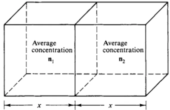
This conclusion can be demonstrated as follows. We consider a situation in which there is a concentration gradient in one direction only, as in the case of diffusion along the length of a long tube or cell. There will be some average distance χ which a molecule will diffuse along the tube in time /. If we take a reference cross section, then, as illustrated in Fig. 2-11, half of the molecules within a distance χ on either side will cross the reference plane in time t. The diffusional flow from left to right is therefore \η^λχ, while that from right to left is \n²x. In the cgs system both are in moles per square centimeter per second.

Since n² = n^x + x(dn/dx), where dn/dx is the concentration gradient, the net flux across the reference plane is

T

lrl

\ i

J

= ih

> * - τ ( *

Λ )J = " 2 7 Λ ·

-

Comparison with Eq. (2-65) gives

(2-67) Equation (2-67) allows a very simple derivation of 3f from kinetic molecular theory. Although the displacement χ can be the net result of many random steps, it can also be put equal to the smallest step which is random with respect to succeeding ones. This smallest step is the mean free path distance λ. During such a step the molecule is moving with velocity c, so the average time between steps is just λ/c. On substituting χ = X and t = X/c into Eq. (2-67) we get

a = \Xc. (2-68)

Example. Drawing o n the preceding example, for oxygen at 25°C a n d 1 a t m , 2 — (1/2) (7.016 χ 10-«)(4.442 χ 10⁴) = 0.156 c m² sec"¹. Alternatively, in SI units, 9 = 1.56 χ 10"⁵ m² s e c^{- 1}.

Equation (2-68) applies to the interdiffusion of molecules of a single kind. Such a diffusion is called self-diffusion, and can be measured experimentally by the use of isotopic labeling. That is, in the experiment corresponding to Fig. 2-11, there can be no overall pressure gradient since otherwise there would be a wind or viscous

FIG. 2 - 1 0 . Random walk. F I G . 2 - 1 1 . Here n^x and n² are average concentrations.