Moment-type estimates with
asymptotically optimal structure for the accuracy of the normal approximation ∗
Irina Shevtsova
Faculty of Computational Mathematics and Cybernetics Lomonosov Moscow State University, Moscow, Russia
Institute for Informatics Problems of the Russian Academy of Sciences e-mail: ishevtsova@cs.msu.su
Dedicated to Mátyás Arató on his eightieth birthday
Abstract
For the uniform distance ∆n between the distribution function of the standard normal law and the distribution function of the standardized sum of independent random variables X1, . . . , Xn withEXj = 0, E|Xj| = β1,j, EXj2=σ2j,j= 1, . . . , n, for alln>1the bounds
∆n6 2`n
3√
2π+ 1
2√ 2πB3n
Xn j=1
β1,jσ2j+R(`n),
∆n6 inf
c>2/(3√2π)
c`n+K(c) Bn3
Xn j=1
σj3+Rc(`n)
, are proved, where B2n = Pn
j=1σj2, `n = B−n3Pn
j=1E|Xj|3, R(`n) 6 6`5/3n , Rc(`n)6min{3`7/6n , A(c)`4/3n }in the general case andR(`n)63`2n, Rc(`n)6 min{2`3/2n , A(c)`2n}, ifX1, . . . , Xn are identically distributed,A(c)>0being a decreasing function of c such that A(c) → ∞ as c → 2/(3√
2π). More- over, the function K(c) is optimal for each c > 2/(3√
2π). In particular, K (√
10 + 3)/(6√ 2π)
= 0,K 2/(3√ 2π)
= q
(2√
3−3)/(6π) = 0.1569. . . It is shown that in the first inequality the coefficients2/(3√
2π)and 2√ 2π−1
∗Research supported by the Russian Foundation for Basic Research (projects 11-01-00515a, 11-07-00112a, 11-01-12026-ofi-m and 12-01-31125) and by the Ministry for Education and Science of Russia (grant MK–2256.2012.1 and State contract 16.740.11.0133).
Proceedings of the Conference on Stochastic Models and their Applications Faculty of Informatics, University of Debrecen, Debrecen, Hungary, August 22–24, 2011
241
are optimal and the lower bound 2/(3√
2π) for c in the second inequal- ity is unimprovable. These results sharpen the well-known estimates due to H. Prawitz (1975), V. Bentkus (1991, 1994) and G. P. Chistyakov (1996, 2001). Also, an analog of the first inequality is proved for the case where the summands possess only the moments of order2 +δwith some0< δ <1. As a by-product, the von Mises inequality for lattice distributions is sharpened and generalized.
Keywords: central limit theorem, convergence rate estimate, normal approx- imation, Berry–Esseen inequality, asymptotically exact constant, character- istic function
MSC: 60F05, 60E10
1. Introduction
Forδ∈[0,1]letF2+δ be the class of distribution functions (d.f.’s)F(x)satisfying the conditions
+∞Z
−∞
x dF(x) = 0,
+∞Z
−∞
|x|2+δdF(x)<∞.
Forh >0 letF2+δh denote the class of all lattice d.f.’s from F2+δ with spanh. For F ∈ F2+δ set
βr=βr(F) =
+∞
Z
−∞
|x|rdF(x), 0< r62 +δ, σ2=β2.
Forδ = 0 by F2 we mean the class of all d.f.’s with zero mean and finite second moment. It is easy to see that F2+δ1 ⊂ F2+δ2 for any 0 6 δ1 < δ2 6 1, and σ2+δ 6β2+δ for allF ∈ F2+δ andδ∈[0,1]by the Lyapounov inequality.
LetX1, . . . , Xn be independent random variables (r.v.’s) defined on some prob- ability space(Ω,A,P)with the corresponding d.f.’sF1, . . . , Fn∈ F2+δ. Denote
σ2j =EXj2, βr,j=E|Xj|r, 0< r62 +δ, j = 1,2, . . . , n, Bn2=
Xn j=1
σ2j, `n= 1 Bn2+δ
Xn j=1
β2+δ,j,
Fn(x) =P(X1+. . .+Xn < xBn) = (F1∗. . .∗Fn)(xBn),
∆n= ∆n(F1, . . . , Fn) = sup
x |Fn(x)−Φ(x)|, n= 1,2, . . . ,
Φ(x)being the standard normal d.f. Assume, thatBn >0. It is easy to verify that under the above assumptions for anyn>1we have
`n > 1 B2+δn
Xn j=1
σj2+δ >n−δ/2.
If the r.v.’sX1, . . . , Xnare independent and identically distributed (i.i.d.), then their common d.f. will be denoted by F (=F1 =. . . =Fn). In this case we use the notation
∆n(F) = ∆n(F1, . . . , Fn), σ2=EX12>0, β2+δ=E|X1|2+δ, βδ=E|X1|δ. Then
Bn=σ√
n, `n = β2+δ
σ2+δnδ/2.
In what follows, for a r.v. X the notation X ∈ F2+δ means that the d.f.
F(x) =P(X < x),x∈R, belongs to the classF2+δ.
As is known, the rate of convergence in the central limit theorem of probability theory obeys the Berry–Esseen inequality
∆n6Cbe(δ)·`n, n>1, F1, . . . , Fn∈ F2+δ, (1.1) where Cbe(δ) depends only on δ [4, 8, 9]. Omitting the history of improvement of the constant Cbe(1) the details of which can be found, for example, in the papers [19, 20], note that
0.4097. . .=
√10 + 3 6√
2π 6Cbe(1)6
( 0.5600, in the general case, 0.4784, ifF1=. . .=Fn,
see [10, 28, 20].1 In 1966–1967 V. M. Zolotarev [37, 38, 39] suggested thatCbe(1) = (√
10 + 3)/(6√
2π). This hypothesis has been neither proved nor rejected yet.
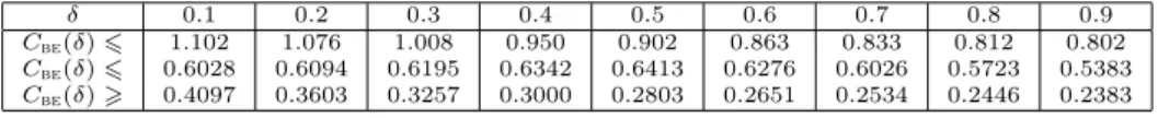
For 0 < δ < 1 the best known upper estimates of the constants Cbe(δ) were obtained by W. Tysiak [30] for the general case (the second line in table 1) and by M. Grigorieva and I. Shevtsova [13] for the case of identically distributed summands (the third line in table 1). The first lower estimates were recently obtained by the author [29] (the fourth line in table 1).
In the case of identically distributed summands (F1=. . .=Fn=F) andδ= 1, inequality (1.1) takes the form
∆n6Cbe(1)· β3
σ3√n, n>1, F ∈ F3, (1.2) and along with the information concerning the two first moments also uses the value of the third absolute momentβ3.
1Recently, the presented upper bounds forCbe(1)were improved toCbe(1)60.5591 in the general case by Ilya Tyurin (see “An improvement of the remainder in the Lyapounov theorem”, Theory Probab. Appl., 2011, vol. 56, No. 4, p. 808-811 (in Russian)) and toCbe(1)60.4748in the i.i.d.-case by the author (see “On the absolute constants in the Berry–Esseen type inequalities for identically distributed summands”, arXiv:1111.6554, 28 November 2011), the latest one — as a corollary to the estimate with an improved structure ∆n 6 0.33554(β3/σ3+ 0.415)/√n, since0.33554(β3/σ3+ 0.415)60.33554·0.415β3/σ3<0.4748β3/σ3 by virtue of the Lyapounov inequality. Independently, an estimateCbe(1)6 0.4774 for the i.i.d.-case was obtained in the paper of I. Tyurin.
δ 0.1 0.2 0.3 0.4 0.5 0.6 0.7 0.8 0.9 Cbe(δ)6 1.102 1.076 1.008 0.950 0.902 0.863 0.833 0.812 0.802 Cbe(δ)6 0.6028 0.6094 0.6195 0.6342 0.6413 0.6276 0.6026 0.5723 0.5383 Cbe(δ)> 0.4097 0.3603 0.3257 0.3000 0.2803 0.2651 0.2534 0.2446 0.2383
Table 1: Two-sided estimates of the constantsCbe(δ)from inequal- ity (1.1) for someδ∈(0,1). The second line: the upper estimates in the general case [30]; the third line: improved estimates for the case of identically distributed summands [13]; the fourth line: the
lower estimates [29].
On the other hand, as n→ ∞, if the summands are i.i.d. with arbitraryfixed (independent ofn) d.f. F ∈ F3, then, as it was established in 1945 by Esseen [9], uniformly inx
Fn(x) = Φ(x) +EX13
6σ3 ·(1−x2)e−x2/2
√2πn +h
σ·Hn(x)e−x2/2
√2πn +o 1
√n
, (1.3) whereh=hHn(x)≡0, ifF is non-lattice, and
Hn(x) = 1 2−n
x√ n−an
σ σ
h
o, |Hn(x)|61 2,
ifF is concentrated on the lattice {a+kh, k = 0,±1,±2, . . .} with span h, {x} being the fractional part ofx∈R, whence Esseen deduced [10] that
lim sup
n→∞ ∆n(F)√
n=|EX13|+ 3hσ2 6√
2πσ3 , F ∈ F3h. (1.4) So, unlike (1.2), in the asymptotic relations (1.3) and (1.4) the third absolute moment E|X1|3 does not take part at all whereas only the first three original moments are used as well as the parameter h, carrying the information on the structureof the basic distribution. The numerical characteristics mentioned above satisfy the relation [10, 40]
sup
h>0
sup
X∈F3h
|EX3|+ 3hEX2 E|X|3 =√
10 + 3, (1.5)
with supremum attained at the two-point distribution P(X =−h(4−√
10)/2) = (√
10−2)/2,P(X =h(√
10−2)/2) = (4−√
10)/2, calledthe Esseen distribution.
From (1.4) and (1.5) it follows that for anyF ∈ F3 lim sup
n→∞ ∆n(F)√ n6
√10 + 3 6√
2π ·β3
σ3. (1.6)
With the supremum attained at the Esseen distribution. This remark makes it possible to establish the lower estimate Cbe(1) > (√
10 + 3)/(6√
2π) as it was done by Esseen [10]. It is worth noticing for the sake of completeness that the
normalized value of the third absolute moment of the Esseen distribution delivering the extremum in (1.5) and equality in (1.6) have the form
β3/σ3= q
20(√
10−3)/3 = 1.0401. . .
So, if in (1.5) the supremum is sought not over all X ∈ F3h, but under additional requirement that the ratio E|X|3/(EX2)3/2 should be large enough, then the ex- tremal value becomes smaller and hence, the lower estimate of the constantCbe(1) in (1.2) becomes more optimistic. This remark generates the hope (and explains) that the larger the value of the Lyapounov ratio β3/σ3, the smaller the upper estimate of the constantCbe(1)in (1.1) is.
Apparently, S. Zahl was the first to notice this [35, 36]. In 1963 he presented the structural improvement of inequality (1.1)
∆n6 0.651 Bn3
Xn j=1
β3,j0 , where
β03,j=
( β3,j, β3,j>3σ3j/√ 2, σj3/ 0.7804−0.1457β3,j/σj3
, β3,j<3σ3j/√ 2,
which more efficiently uses the information concerning the first three moments of random summands.
The next step in this direction was made in 1975 by H. Prawitz, from whose paper [25] one can deduce the estimate
∆n 6`n·A1(`n) + 1 2√
2πBn3 Xn j=1
σj3+ 1 4πBn4
Xn j=1
σj4, (1.7) whereA1(`)is a positive function of` >0 with a complicated structure such that A1(`)does not increase for`small enough and
`→0limA1(`) =1.0253 6√
2π + 1 2√
2π = 2 3√
2π+0.0253 6√
2π = 0.2676. . .
Prawitz also described an algorithm for the computation of A1(`) for concrete values of`. Since
1 Bn3
Xn j=1
σj36 1 Bn3
Xn j=1
β3, j=`n, 1 Bn4
Xn j=1
σj46`4/3n =o(`n), `n→0, from (1.7) it follows that
∆n6`n·A2(`n), (1.8)
whereA2(`)is a positive function of ` >0 such thatA2(`)does not increase for ` small enough and
`lim→0A2(`) =1.0253 6√
2π + 1
√2π = 7 6√
2π+0.0253 6√
2π = 0.4671. . . .
Inequality (1.8) with concrete values ofA2 plays an important role in the problem of determination of upper estimates of the absolute constantCbe(1)in the Berry–
Esseen inequality (1.1), since the algorithms which are traditionally used for these purposes cannot obtain the values of this constant which are less thanA2.
In the same paper [25], for identically distributed summands andn>2, Prawitz announced the inequality
∆n6 2 3√
2π· β3
σ3√
n−1 + 1
2p
2π(n−1)+A3·`2n−1, (1.9) whereA3 is an absolute positive constant and stated that the coefficient
2 3√
2π = 0.2659. . .
at the Lyapounov fraction in (1.9) cannot be made smaller. Unfortunately, the proof of this statement as well as that of inequality (1.9) were not published by Prawitz.
A strict proof of Prawitz’ inequality (1.9), however, with a little worse remain- der, follows from the papers of V. Bentkus [2, 3], in which for the case of arbitrary F1, . . . , Fn∈ F3 andn>1 the estimate
∆n6 2`n
3√
2π + 1 2√
2πBn3 Xn j=1
σj3+A4·`4/3n 6 7`n
6√
2π+A4·`4/3n (1.10) was obtained, whereA4is an absolute constant. The worse order of the remainder in (1.10) as compared with (1.9) is due to that the estimate (1.10) holds for arbitrary (not necessarily identical)F1, . . . , Fn ∈ F3.
So, even if the value of the constant A4 in (1.10) were known, it would not be possible to obtain an estimate of the absolute constantCbe(1)in the Berry–Esseen inequality (1.1) lower than 7/(6√
2π) = 0.4654. . . . For further progress in this problem, one has to improve the main term of asymptotic estimate (1.10).
In 1953 A. N. Kolmogorov [17] (also see the monographs of I. A. Ibragimov and Yu. V. Linnik [16] and V. M. Zolotarev [40]) formulated the problem of calculation of the so-called asymptotically exact constant
Cae= lim sup
`→0
sup
n>1, F1,...,Fn:`n=`
∆n(F1, . . . , Fn)
` ,
for which from the papers of Esseen [10] and Bentkus [2, 3] it follows that 0.4097. . .=
√10 + 3 6√
2π 6Cae6 7 6√
2π = 0.4654. . . .
V. M. Zolotarev [38, 39, 40] held the opinion thatCaecoincides with its lower bound and together with A. N. Kolmogorov considered the problem of calculation ofCaeto
be intermediate or auxiliary for the problem of calculation of the exact value of the absolute constantCbe(1)in (1.1). The gap of approximately 0.06 between the upper and lower bounds of Cae presented above is due to the fact that the information on theoriginalmoments of summands is not taken into account in [25, 2, 3]. Since the summands are centered, the only informative original moment is the third one.
S. V. Nagaev and V. I. Chebotarev [21] also noticed this and for the i.i.d. two-point summands proved the estimateCbe(1)60.4215.
In 2001–2002 G. P. Chistyakov [7] obtained a new asymptotic expansion general- izing that due to Esseen (1.3) to the case of non-identically distributed summands.
This new expansion allowed Chistyakov, as an intermediate step, to use the in- formation concerning the original moments and other characteristics of the initial distributions and, as a result, to deduce the estimate
∆n6
√10 + 3 6√
2π ·`n+A5·`40/39n |ln`n|7/6, (1.11) whereA5 is an absolute constant. From (1.11) it follows that
Cae=
√10 + 3 6√
2π = 0.4097. . . ,
thus Chistyakov proved the validity of Zolotarev’s hypothesis concerning the exact value of the asymptotically exact constantCae.
Unfortunately, the particular value of the absolute constantA5 in Chistyakov’s inequality (1.11) was not given, so this fundamental result cannot be used for practical calculations, in particular, for the evaluation of the absolute constant Cbe(1)in the Berry–Esseen inequality.
Nevertheless, the inequalities of Prawitz (1.9) and Bentkus (1.10) are interesting because in these inequalities the coefficient at the Lyapounov fraction is less than in Chistyakov’s inequality (1.11):
0.2659. . .= 2 3√
2π <
√10 + 3 6√
2π = 0.4097. . . , and hence, with large values of the ratio
Xn j=1
β3, j
Xn
j=1
σj3
inequalities (1.9) and (1.10) are more precise than (1.11). This ratio may be arbi- trarily large even in the case of identically distributed summands, for example, in the double array scheme whereβ3/σ3=β3(n)/σ3(n)→ ∞, so that
1 B3n
Xn j=1
σ3j = 1
√n =o(`n) as `n= β3(n) σ3(n)√n →0.
So, the unproved Prawitz’ assertion that the coefficient2/(3√
2π)at the Lyapounov fraction is unimprovable becomes exceptionally important. This assertion was proved only recently in [29] where the so-called lower asymptotically exact con- stant
Cae= lim sup
`→0 lim sup
n→∞ sup
F:β3=σ3`√ n
∆n(F)
`
was introduced (for the scheme of summation of identically distributed summands), which is an obvious lower bound for the coefficient under discussion, and it was demonstrated thatCae= 2/(3√
2π).
The unimprovability of the first term in (1.9) naturally puts forward the ques- tion concerning the accuracy of the second term. No suggestions concerning the
“exactness” of the coefficient at the second term in (1.9), (1.10) were stated by Prawitz or Bentkus. Actually, this question can be formulated in an even more general form: for any c > Cae find the least possible value K(c) providing the validity of the asymptotic estimate
sup
F∈F3:β3=ρσ3
∆n(F)6 cρ
√n+K(c)
√n +rn(ρ)· ρ
√n, n, ρ>1, in which the remainderrn(ρ)>0 satisfies the conditions
lim sup
`→0 lim sup
n→∞ rn(`√
n) = 0, sup
ρ>1lim sup
n→∞ rn(ρ) = 0. (1.12) Apparently, for the first time this question was formulated in [29], where lower estimates of K(c) were presented forCae 6 c 6Cae. In particular, for c = Cae in [29] it was shown that
K 2
3√ 2π
>
s 2√
3−3
6π = 0.1569. . . , which is strictly less than the value of the coefficient 2√
2π−1
= 0.1994. . .at the second term in inequalities (1.9) and (1.10). Thus, the question of the “exactness”
of the second term in (1.9) and (1.10) remained unanswered.
In the present paper we will prove that: for all n>1andF1, . . . , Fn∈ F3
∆n6 inf
c>Cae
c`n+K(c) B3n
Xn j=1
σ3j + minn
2.7176`7/6n , A(c)`4/3n o , and for identically distributed summands
∆n 6 inf
c>Cae
cβ3
σ3√n+K(c)
√n + minn
1.7002`3/2n , A(c)`2no ,
with the function K(c)optimal for each c >Cae (the optimality of this function is proved in remark 4.16), A(c) > 0 being a decreasing function of c such that
A(c)→ ∞asc→2/(3√
2π). The functionK(c)decreases monotonically alternat- ing its sign in a single point c = (√
10 + 3)/(6√
2π). So, the second term in the estimates presented above is negative forc >(√
10 + 3)/(6√
2π). The presence of a negative summand in the main term is rather unusual in estimates of the accuracy of the normal approximation, but makes it possible to obtain asymptotically exact estimates as simple corollaries of the results presented above even for symmetric Bernoulli distributions (see corollary 4.19) which distinguishes these results from previously known. In particular, forc=Caewe have
∆n6
√10 + 3 6√
2π ·`n+ 3.4314·`4/3n , n>1, F1, . . . , Fn∈ F3,
∆n6
√10 + 3 6√
2π · β3
σ3√n+ 2.5786·`2n, n>1, F1=. . .=Fn∈ F3,
which improves Chistyakov’s inequality (1.11) with respect to the remainder, whe- reas forc=Caewe have
∆n6 2`n
3√ 2π +
s 2√
3−3 6π
Xn j=1
σj3
Bn3 + 2.7176·`7/6n , n>1, F1, . . . , Fn∈ F3,
∆n6 2 3√
2π · β3
σ3√n+ s
2√ 3−3
6πn + 1.7002·`3/2n , n>1, F1=. . .=Fn∈ F3, which improves Prawitz’ and Bentkus’ inequalities (1.9), (1.10) with respect to the second term. Moreover, we will obtain the absolute improvements of Prawitz’ and Bentkus’ inequalities (1.9) and (1.10):
∆n 6 2`n
3√
2π+ 1 2√
2πB3n Xn j=1
β1,jσ2j+ 5.4527·`5/3n , n>1, F1, . . . , Fn∈ F3,
∆n6 2 3√
2π· β3
σ3√n+ 1 2√
2π· β1
σ√n+ 2.4606·`2n, n>1, F1=. . .=Fn ∈ F3, in which the remainders have no worse order of decrease than in (1.9) and (1.10) but with specified constants and an improved functionPn
j=1β1,jσ2j 6Pn
j=1σ3j of the two first moments in the second term with the same coefficient as in (1.9), (1.10).
Below it will be shown that the value of the coefficient 2√ 2π−1
at this improved function of the two first moments yet cannot be made less (see remark 4.9). As well, similar estimates will be obtained for the case0< δ < 1, generalizing and sharp- ening the results of [11], where only the case of identically distributed summands was considered.
To prove the main results we use a combination of the method of character- istic functions (ch.f.’s) with the truncation method as well as some methods of convex analysis based on the works of W. Hoeffding [15] and V. M. Zolotarev [40].
It is worth noticing that in the preceding works dealing with the accuracy of the normal approximation, Prawitz’ smoothing inequality was used, besides Prawitz himself, only by V. Bentkus [2, 3]. G. P. Chistyakov in [7] used Esseen’s traditional smoothing inequality with the normal smoothing kernel, while in Prawitz’ inequal- ity, the smoothing function has a compact Fourier transform and does not have any probabilistic interpretation.
The paper is arranged as follows. In the second section we present new estimates for ch.f.’s implying, in particular, a generalization and improvement of the von Mises inequality for lattice distributions: for anyh >0,δ∈(0,1]and F∈ F2+δh
h
σ 6 β2+δ
σ2+δ + βδ
σδ,
whereas in the original von Mises inequalityδ= 1and on the right-hand side there is2β3/σ3. In the third section a moment inequality is proved which improves (1.5) and plays the key role for the construction of the optimal function of moments in the resulting estimates. In the fourth section we formulate and prove new moment-type estimates of the accuracy of the normal approximation with optimal structure.
2. Estimates for characteristic functions
Denote
εn =Bn−(2+δ) Xn j=1
(β2+δ,j+βδ,jσ2j) =`n+B−n(2+δ) Xn j=1
βδ,jσj2,
fj(t) =EeitXj, j= 1,2, . . . , n, fn(t) = Yn j=1
fj
t Bn
, rn(t) =fn(t)−e−t2/2, t∈R.
As is well-known, ifX1, . . . , Xn are identically distributed, then fn(t) =
f1
t σ√n
n
, t∈R.
In this section new estimates for|fn(t)|andrn(t)will be obtained.
Letθ0(δ)be the unique root of the equation
δθ2+ 2θsinθ+ 2(2 +δ)(cosθ−1) = 0
within the interval(0,2π). As this is so,π < θ0(δ)<2πfor all0< δ61. Let κδ ≡sup
x>0
cosx−1 +x2/2
x2+δ = cosθ0(δ)−1 +θ02(δ)/2
θ02+δ(δ) = θ0(δ)−sinθ0(δ) (2 +δ)θ01+δ(δ) . (2.1)
Obviously,
κδ6 1
2θ0δ(δ) 6 1
2πδ 61/2, 0< δ61. (2.2) Forε >0let
ψδ(t, ε) =
t2/2−κδε|t|2+δ, |t|< θ0(δ)ε−1/δ, 1−cos ε1/δt
ε2/δ , θ0(δ)6ε1/δ|t|62π, 0, |t|>2πε−1/δ.
It is easy to see that the function ψδ(t, ε) decreases monotonically in ε for each fixedt∈Rand all0< δ61. Moreover,ψδ(t, ε)>0for allt∈R.
The following lemma plays the key role for the construction of estimates of the absolute value of a ch.f.
Lemma 2.1 (see [26]). For any x∈Randθ0(δ)6θ62π cosx61−a(δ, θ)x2+b(δ, θ)|x|2+δ, where
a(δ, θ) = 2 +δ
δ ·1−cosθ θ2 −1
δ· sinθ θ , b(δ, θ) =2
δ ·1−cosθ θ2+δ −1
δ· sinθ θ1+δ. Theorem 2.2. For any F1, . . . , Fn ∈ F2+δ and anyt∈R
|fn(t)|6h 1− 2
nψδ(t, εn)in/2
6exp{−ψδ(t, εn)}6exp
−t2/2 +κδεn|t|2+δ . Proof. LetXj0 be an independent copy of the r.v. Xj,j= 1, . . . , n. Then
fn(t)2= Yn j=1
fj
t Bn
2
= Yn j=1
Ecost(Xj−Xj0)
Bn .
Using lemma 2.1 and relations E(Xj−Xj0)2 = 2σj2, E|Xj−Xj0|2+δ 62 β2+δ,j+ βδ,jσj2
(see, e. g., [34, p. 74, lemma 2.1.7]) we obtain
|fn(t)|26 Yn j=1
1−a(δ, θ)t2E(Xj−Xj0)2
Bn2 +b(δ, θ)|t|2+δE|Xj−Xj0|2+δ Bn2+δ
!
6 Yn j=1
1−2a(δ, θ)t2σ2j
B2n + 2b(δ, θ)|t|2+δβ2+δ,j+βδ,jσ2j Bn2+δ
! .
The expression in brackets is an upper bound for the squared absolute value of the ch.f. fj(t) and, hence, is nonnegative. Since the geometric mean of nonnegative
numbers is no greater than their arithmetic mean, for allt∈Randθ∈[θ0(δ),2π]
we obtain
|fn(t)|26 1− 2
n Xn j=1
a(δ, θ)t2σ2j
B2n −b(δ, θ)|t|2+δβ2+δ,j+βδ,jσj2 B2+δn
! n
=h 1− 2
n a(δ, θ)t2−b(δ, θ)εn|t|2+δ in
≡h 1− 2
nψδ(t, εn, θ)in
, where
ψδ(t, ε, θ) =a(δ, θ)t2−b(δ, θ)ε|t|2+δ, t∈R, ε >0, θ0(δ)6θ62π.
It can be made sure (see, e. g., [26]) that for any fixedt∈Rthe minimum of the right-hand side of the last estimate for|fn(t)|2 is attained at
θ= minn maxn
θ0(δ), ε1/δn |t|o ,2πo
, and
ψδ(t, ε) = max
θ0(δ)6θ62πψδ(t, ε, θ)>ψδ(t, ε, θ0(δ)) =t2/2−κδε|t|2+δ, whence follows the statement of the lemma.
Forn= 1 from theorem 2.2 we obtain
Corollary 2.3. For any r.v. X ∈ F2+δ for allt∈Rthere hold the estimates EeitX261−2ψδ σt, β2+δ/σ2+δ+βδ/σδ61−σ2t2+ 2κδ β2+δ+βδσ2
|t|2+δ. Remark 2.4. For δ = 1, in the paper of H. Prawitz [24] the first inequality of corollary 2.3 is proved as well as the second inequality of theorem 2.2. In the book of N. G. Ushakov [34] the second inequality of corollary 2.3 is proved for arbitrary 0< δ61.
Remark 2.5. From corollary 2.3 it follows that |f(t)|<1 for |t| < 2π(β2+δ/σ2+ βδ)−1/δfor any d.f. F ∈ F2+δ. A special role of the pointt= 2π(β2+δ/σ2+βδ)−1/δ is due to the fact that this is the least possible period of the ch.f. of a r.v. with fixed three absolute momentsβδ, σ2 and β2+δ. Indeed, for the symmetric distribution P(X = ±a) = 1/(2a2), P(X = 0) = 1−1/a2 with a = 1/√
2δ−1 we have βδ =aδ−2, σ2= 1, β2+δ =aδ. It is easy to see that the ch.f. f(t) =Ecos(tX) = 1−(1−cos(at))/a2equals 1fort=π/a, and withaspecified above
π
a = 2π
a(1 +a−2)1/δ = 2π (β2+δ+βδ)1/δ.
The fact mentioned in remark 2.5 can be used for the improvement of the von Mises inequality
h σ 62β3
σ3,
relating the span of a lattice distribution with its moments. Namely, from corol- lary 2.3 it follows that
t0= inf{t >0 :|f(t)|= 1}>2π(β2+δ/σ2+βδ)−1/δ.
As is known, t0 <∞ if and only if F ∈ F2+δh withh = 2π/t0. So, the following theorem holds.
Theorem 2.6. For any h >0and X∈ F2+δh
h6(β2+δ/σ2+βδ)1/δ. (2.3) For all 0< δ 61, this inequality is unimprovable in the sense that for any h >0 we have
supn
h(β2+δ/σ2+βδ)−1/δ:X ∈ F2+δh
o= 1, 0< δ 61,
moreover, the supremum is attained at the family of distributions of the form P
X = h
1 +u
= u
1 +u= 1−P
X =− uh 1 +u
, u→ ∞.
Forδ= 1the supremum is also attained at the extremal distributionP(X =h/2) = P(X =−h/2) = 1/2.
Theorem 2.2 and inequality (2.3) also improve the results of paper [26], in which σδ >βδ is used instead ofβδ.
Lemma 2.7. For any F1, . . . , Fn∈ F2+δ andt∈R rn(t)≡fn(t)−e−t2/2
6 Xn j=1
fj
t Bn
−exp (
−σj2t2 2Bn2
)exp (
−t2
2 1− σj2 Bn2
!
+κδεn|t|2+δ )
. Proof. In [25] it was proved that for anyAj >0,Bj∈C,Cj>max{Aj,|Bj|}
Yn j=1
Bj− Yn j=1
Aj
6 1
2 Yn i=1
Ci
Xn j=1
|Bj−Aj| Cj
+1 2
Yn i=1
Ai
Xn j=1
|Bj−Aj| Aj
6 Xn j=1
|Bj−Aj| Aj
Yn i=1
Ci. Using this inequality with
Bj=fj
t Bn
, Aj= exp (
−σ2jt2 2Bn2
) ,
Cj = exp (
−σ2jt2
2B2n +κδ(β2+δ,j+βδ,jσj2)|t|2+δ Bn2+δ
)
(the estimate|Bj|6Cj follows from theorem 2.2), forrn(t)we obtain
rn(t) =
Yn j=1
fj
t Bn
− Yn j=1
exp (
−σ2jt2 2B2n
) 6
6 Xn j=1
fj
t Bn
−exp (
−σ2jt2 2Bn2
)exp (
−t2
2 +κδεn|t|2+δ+σj2t2 2Bn2
) . The way we estimate|fj(t/Bn)−e−σ2jt2/(2Bn2)|in lemma 2.7 depends on whether δ= 1 or not.
Lemma 2.8. For any r.v. X∈ F2+δ with the ch.f. f(t)for allt∈Rwe have the estimates:
ifδ= 1, then
f(t)−e−σ2t2/26 β3|t|3
6 , (2.4)
f(t)−e−σ2t2/26 |t|3
6 EX31(|X|6U)+E|X|31(|X|> U) + + t4
24E|X|41(|X|6U) +σ4t4
8 (2.5)
for allU >0;
if0< δ61, then
f(t)−e−σ2t2/26γδβ2+δ|t|2+δ+σ4t4/8, (2.6) where
γδ = sup
x>0
eix−1−ix−(ix)2/2/x2+δ
= sup
x>0
scosx−1 +x2/2 x2+δ
2
+
sinx−x x2+δ
2
.
The values of γδ for some 0 < δ 6 1 are presented in the second column of table 3. In particular, γ1 = 1/6. The estimates given in lemma 2.8 were appar- ently first obtained for the case 0 < δ < 1 by W. Tysiak [30]. Nevertheless, for completeness we give their simple proof as well.
Proof. The first estimate follows from the works of I. Tyurin [31, 32], in which the inequality
f(t)−e−σ2t2/26e−t2/2
|t|
Z
0
β3s2
2 es2/2ds6
|t|
Z
0
β3s2
2 ds=β3|t|3
6 , t∈R,
was proved.
Further, using the inequality |e−x−1 +x| 6 x2/2, x > 0, for all t ∈ R we obtain
|f(t)−e−σ2t2/2|6E
eitX−1−itX+t2X2 2
+
e−σ2t2/2−1 +σ2t2 2
6R(t) +σ4t4
8 , where
R(t) = E
eitX−1−itX−(itX)2 2
6R1(t, U) +R2(t, U), R1(t, U) =
E
eitX−1−itX−(itX)2 2
1(|X|6U) , R2(t, U) =E
eitX−1−itX−(itX)2 2
1(|X|> U) for anyU >0.
By the definition of γδ,eix−1−ix−(ix)2/26γδ|x|2+δ, x∈R, whence for R2(t, U)we obtain
R2(t, U)6γδ|t|2+δE|X|2+δ1(|X|> U).
Adding and subtracting (itX)3/6 · 1(|X| 6 U) under the sign of expectation in R1(t, U), taking account of the inequality eix−1−ix−(ix)2/2−(ix)3/6 6 x4/24,x∈R, forR1(t, U)we obtain
R1(t, U)6E
eitX−1−itX−(itX)2
2 −(itX)3 6
1(|X|6U) +|t|3
6
EX31(|X|6U)6 t4
24EX41(|X|6U) +|t|3 6
EX31(|X|6U). So, for any0< δ61andU >0 for allt∈Rwe have
|f(t)−e−σ2t2/2|6σ4t4
8 +γδ|t|2+δE|X|2+δ1(|X|> U) +|t|3
6
EX31(|X|6U)+ t4
24EX41(|X|6U).
Setting U = 0 in this inequality, we obtain the second estimate of the lemma, settingδ= 1 we obtain the third one. The lemma is completely proved.
Remark 2.9. Note that using new optimal estimates forζ-metrics obtained in [33], we can as well prove an analog of the first estimate of lemma 2.8 for the case of an arbitrary0< δ <1 in the form
f(t)−e−t2/26 β2+δ|t|2+δ (1 +δ)(2 +δ)sup
x>0
|eix−1| xδ ,
however, it turns out that for all0< δ <1 1
(1 +δ)(2 +δ)sup
x>0
|eix−1| xδ >sup
x>0
eix−1−ix−(ix)2/2 x2+δ =γδ,
that is, the coefficient atβ2+δ|t|2+δ in this estimate will be greater than that in the third estimate of lemma 2.8. This circumstance is critical for the estimation of the remainder in the central limit theorem since it is this coefficient that determines the value of the constant at the main term. This is the reason why the third estimate of lemma 2.8 is more preferable, and will be used for our purposes.
3. The moment inequality
Theorem 3.1. For any r.v. X ∈ F3, for allλ>1 the inequality
|EX3|+ 3E|X| ·EX26λE|X|3+M(p(λ), λ)(EX2)3/2 holds, where
p(λ) = 1 2−
rλ+ 1 λ+ 3sin
π 6 −1
3arctan r
λ2+ 2λ−1 λ+ 3
, M(p, λ) =1−λ+ 2(λ+ 2)p−2(λ+ 3)p2
pp(1−p) , 0< p61
2, λ>1,
with equality attained for each λ > 1 at the family of two-point distributions P X = σp
q/p
= p = 1−P X = −σp p/q
: σ > 0 , where p = p(λ), q= 1−p(λ).
The optimal values of the parameter λ = λ(β3), delivering the minimum to the right-hand side of the inequality in theorem 3.1 and the corresponding values p=p(λ(β3))are presented for someβ3=E|X|3/(EX2)3/2in the fourth and seventh columns, respectively, of table 2 below.
Remark 3.2. It can be made sure that the function p(λ) increases monotonically forλ>1, varying within the limits
0.3169. . .= 1 2
1−
q 1−√
3/2
=p(1)6p(λ)6 lim
λ→∞p(λ) = 1 2.
Moreover, as it will be seen from the proof, the functionM(p(λ), λ)can be repre- sented as
M(p(λ), λ) = sup
0<p61/2
(α3(p)−λβ3(p) + 3β1(p)),
where α3(p), β3(p), β1(p)are, respectively, the third original, third absolute and first absolute moments of the Bernoulli distribution assigning the probabilitiesp andq= 1−pto the pointsp
q/pand−p p/q: M(p(λ), λ) = sup
q−p−λ(p2+q2) + 6pq
√pq : 0< p61
2, q= 1−p
. (3.1)
From this representation, first, it follows that the functionM(p, λ)decreases mono- tonically in λ > 1 for each 0 < p 6 1/2. The same property is inherent in M(p(λ), λ), since for anyλ1>λ2>1we have
M(p(λ1), λ1)6M(p(λ1), λ2)6 sup
0<p<1/2
M(p, λ2) =M(p(λ2), λ2).
Second, evidently,
M(p(λ), λ)>q−p−λ(p2+q2) + 6pq
√pq
p=q=1/2
= 3−λ, λ>1, with equality attained atλ→ ∞, so that
λinf>1 λ+M(p(λ), λ)
= lim
λ→∞ λ+M(p(λ), λ)
= 3.
Thus, the functionM(p(λ), λ)decreases monotonically for allλ>1, varying within the limits
2.3599. . .= 2 q
3√
3(2−√
3) =M(p(1),1)>M(p(λ), λ)>lim
λ→∞M(p(λ), λ) =−∞, whence it follows that M(p(λ), λ) alters its sign at the unique point λ = √
10 corresponding to the valuep(√
10) = 2−√
10/2 = 0.4188. . . ,so that M(p(λ), λ)<0 ⇐⇒ λ >√
10.
Since p2+q2−√pq = −2pq−√pq+ 1 > 0 for all p∈ (0,1/2), q = 1−p, from (3.1) it also follows that the function
λ+M(p(λ), λ) = sup
q−p−λ(p2+q2−√pq) + 6pq
√pq : 0< p6 1
2, q= 1−p
decreases monotonically, varying within the limits 3< λ+M(p(λ), λ)61 + 2
q 3√
3(2−√
3) = 3.3599. . . , λ>1. (3.2) Using theorem 3.1 it is possible to improve a result due to C.-G. Esseen [10], according to which for a sequence of independent r.v.’s X1, X2. . . with the d.f.
F ∈ F3h for someh >0such that EX12= 1, EX13=α3,E|X1|3=β3, the relation ψ(F)≡lim sup
n→∞ ∆n√
n= |α3|+ 3h 6√
2π 6
√10 + 3 6√
2π β3≡ψ1(β3) holds (see (1.4) and (1.6)).
On the other hand, according to (2.3) for hwe have the estimateh6β3+β1, whence it follows that in the case considered by Esseen
ψ(F)6|α3|+ 3(β3+β1) 6√
2π 6 inf
λ>1
(λ+ 3)β3+M(p(λ), λ) 6√
2π =
= inf
c>2/(3√
2π)(cβ3+K(c))≡ψ2(β3), (3.3) where
K(c) = M(p(λ), λ) 6√
2π
λ=6√2πc
−3
.
Moreover, from theorem 3.1 it follows that c cannot be less than 2/(3√ 2π) = 0.2659. . . , and K(c) in (3.3) can be made less for noc > 2/(3√
2π). From (3.3) withc= (√
10 + 3)/(6√
2π) = 0.4097. . . (that corresponds toλ=√
10,K(c) = 0) Esseen’s bound follows, whereas (3.3) with c = 2/(3√
2π) (that corresponds to λ= 1) implies the estimate
ψ(F)6 2 3√
2π·β3+ s
2√ 3−3
6π <0.2660β3+ 0.1570, (3.4) which is more accurate than Esseen’s boundψ(F)6ψ1(β3)for
β3>2 q
3√
3(2−√
√ 3)
10−1 = 1.0914. . . , although the value c = 2/(3√
2π) (that is, λ = 1) is optimal in (3.3) only for β3>1.2185. . .
Comparing the functions ψ1(β3) and ψ2(β3), we conclude that their values coincide only at the unique pointβ3 for which c= (√
10 + 3)/(6√
2π), K(c) = 0 (that corresponds toλ=√
10,p(√
10) = 2−√
10/2), that is, at the point β3= p2+ (1−p)2
pp(1−p) p=2
−√ 10/2
= q
20(√
10−3)/3 = 1.0401. . . ,
and for all the rest of the values of β3 >1 the strict inequality ψ1(β3)> ψ2(β3) holds. In particular, forβ3 = 1(that is, for the symmetric Bernoulli distribution) ψ1(1) = (√
10 + 3)/(6√
2π) = 0.4097. . . ,while ψ2(1) = lim
c→∞(c+K(c)) = lim
λ→∞
λ+ 3 +M(p(λ), λ) 6√
2π
= 1
√2π = 0.3989. . . < ψ1(1)−0.0107.
The values of the functionsψ1(β3)andψ2(β3)for someβ3>1are presented in the second and third columns of table 2. The corresponding values of c =c(β3) and K=K(c(β3))delivering the minimum in (3.3) are presented in the fifth and sixth columns of table 2.
β3 ψ1 ψ2 λ c K p 1 0.4097 0.3989 + inf + inf −inf 1/2 1.01 0.4138 0.4111 7.2034 0.6784 -0.2741 0.4592 1.02 0.4179 0.4170 4.8305 0.5206 -0.1141 0.4424 1.03 0.4220 0.4218 3.7862 0.4512 -0.0430 0.4296 1.04 0.4261 0.4261 3.1682 0.4101 -0.0005 0.4189 1.05 0.4302 0.4300 2.7497 0.3823 0.0286 0.4095 1.06 0.4343 0.4337 2.4432 0.3619 0.0501 0.4011 1.07 0.4384 0.4373 2.2070 0.3462 0.0668 0.3934 1.08 0.4425 0.4407 2.0182 0.3336 0.0803 0.3863 1.09 0.4466 0.4440 1.8633 0.3233 0.0915 0.3796 1.10 0.4507 0.4471 1.7335 0.3147 0.1009 0.3733 1.12 0.4589 0.4533 1.5275 0.3010 0.1161 0.3618 1.14 0.4670 0.4592 1.3707 0.2906 0.1279 0.3513 1.16 0.4752 0.4649 1.2470 0.2823 0.1374 0.3416 1.18 0.4834 0.4705 1.1470 0.2757 0.1451 0.3326 1.20 0.4916 0.4760 1.0645 0.2702 0.1517 0.3243 1.21 0.4957 0.4787 1.0284 0.2678 0.1546 0.3203 1.22 0.4998 0.4813 1.0000 0.2659 0.1569 0.3169 Table 2: The values of the functionsψ1(β3) andψ2(β3) for some β3; optimal values ofc= (λ+ 3)/(6√
2π)delivering the minimum toψ2(β3)(see (3.3)); the corresponding values ofK(c)in (3.3); the
parameterp(λ)of the extremal distribution.
Proof of theorem3.1. Since for σ2 ≡ EX2 = 0 the statement of the theorem is obvious, in what follows we assume thatσ >0. Consider the functional
Jλ,σ(X) = |EX3|+ 3E|X|σ2−λE|X|3
/σ3, X∈ F3. Then the statement of the theorem is equivalent to
sup
σ>0
sup
X∈F3:EX=0,EX2=σ2
Jλ,σ(X) =M(p(λ), λ).
On the other hand, for anyσ >0 sup
X∈F3:EX=0,EX2=σ2
Jλ,σ(X) = sup
X∈F3:EX=0,EX2=σ2
Jλ,σ(−X)
= sup
X∈F3:EX=0,EX2=σ2
Jeλ,σ(X), where
Jeλ,σ(X) = EX3+ 3E|X|σ2−λE|X|3 /σ3.
With the account of the results of W. Hoeffding [15] and V. M. Zolotarev [40] it is easy to see that for each σ > 0 the extremum of the moment-type functional
Jeλ,σ(X)linear with respect to F∈ F3 under two moment-type restrictions EX = 0, EX2=σ2,
is attained on distributions concentrated in at most three points. Without loss of generality assume that the r.v. X takes the values x < y 6 0 < z with the probabilities
P(X =x) = σ2+yz
(z−x)(y−x), P(X =y) =− σ2+xz (z−y)(y−x), P(X=z) = σ2+xy
(z−x)(z−y), −yz6σ26−xz.
Then
E|X|= 2z(σ2+xy)
(x−z)(y−z), 3E|X|σ2= 6zσ4+ 6xyzσ2 (x−z)(y−z), E|X|3=(z3+a)σ2−xyz(xy−xz−yz−z2)
(z−x)(z−y) ,
EX3= (x+y+z)σ2+xyz=(z3−a)σ2+xyz(xy−xz−yz+z2) (z−x)(z−y) , a=a(x, y, z) =z(x2+y2+xy)−xy(x+y)>0, x < y60< z, Jeλ,σ(X) = 6zσ+ (6xyz−(λ−1)z3−a(λ+ 1))σ−1+
+xyz((λ+ 1)(xy−xz−yz)−(λ−1)z2)σ−3
/((z−x)(z−y)) and
sup
σ>0
sup
X∈F3:EX=0,EX2=σ2
Jeλ,σ(X) = sup
X∈F3:EX=0
sup
σ>0
g(σ) (z−x)(z−y), where
g(σ) =g(σ, x, y, z, λ) = 6zσ+ (6xyz−(λ−1)z3−a(λ+ 1))σ−1+ +xyz((λ+ 1)(xy−xz−yz)−(λ−1)z2)σ−3.
Show that the functiong(σ)is quasi-convex forσ >0, namely, eitherg(σ)increases monotonically for σ >0 or there exists a pointσ1 > 0 such that g(σ) decreases monotonically for 0 < σ < σ1 and increases monotonically for σ > σ1. For this purpose differentiateg(σ)and find the stationary points. We have
g0(σ) = 6z+ (a(λ+ 1) + (λ−1)z3−6xyz)σ−2
−3xyz((λ+ 1)(xy−xz−yz)−(λ−1)z2)σ−4>0
if and only if
6σ4+ (a(λ+ 1)/z+ (λ−1)z2−6xy)σ2+ 3xy((λ−1)z2−(λ+ 1)(xy−xz−yz))>0.
So, the equationg0(σ) = 0is equivalent to the quadratic equation with respect to σ2. The latter either has no real roots and theng0(σ)>0 andg(σ)increases, or has one real root which is the point of reflection ofg(σ)and theng(σ)increases, or has two different real rootsσ1 < σ2 so thatσ1 is the point of maximum andσ2 is the point of minimum. The desired property of the functiong will be proved if we show that the smaller rootσ1of the equationg0(σ) = 0is non-positive.
The smaller roots1of the quadratic equations2+bs+c= 0with two different roots has the form s1 =−b−√
b2−4c. It is obvious that s1 6 0 if and only if eitherb >0, orb60andc60, that is, if the conditionb60impliesc60. Apply this reasoning tos=σ2,
b= (a(λ+ 1)/z+ (λ−1)z2−6xy)/6, c= xy
2z((λ−1)z3−(λ+ 1)z(xy−xz−yz)).
Indeed, the conditionb60implies(λ−1)z366xyz−a(λ+ 1)and c· 2z
(λ+ 1)xy 6 6xyz
λ+ 1−a−z(xy−xz−yz)63xyz−a−z(xy−xz−yz) =
=xz(y−x)−y2z+ (x+y)(xy+z2)60
for allλ>1andx < y60< z. So, the maximum value of the functiong(σ)on the interval−yz6σ2 6−xz is attained either atσ2=−yz and thenP(X =x) = 0, or at σ2 =−xz and thenP(X =y) = 0, that is, the extremum of the functional Jeλ,σ(X)is attained at two-point distributions of the r.v. X.
Now letP(X =σp
q/p) =p,P(X =−σp
p/q) =q= 1−p,0< p <1. Then EX3= q−p
√pq σ3, E|X|3= p2+q2
√pq σ3=1−2pq
√pq σ3, E|X|= 2√pqσ.
SinceEX3<0forp <1/2, the range of the values ofpunder consideration can be restricted to the semi-interval(0,1/2]. Further, the functional
Jeλ,σ(X) =EX3−λE|X|3+ 3E|X|σ2
σ3 =q−p−λ(1−2pq) + 6pq
√pq =
= 1−λ+ 2(λ+ 2)p−2(λ+ 3)p2
pp(1−p) ≡M(p, λ)
does not depend onσand hence, sup
σ>0 sup
X∈F3:EX=0,EX2=σ2
Jeλ,σ(X) = sup
0<p61/2M(p, λ).
It remains to show that for eachλ,M(p, λ)attains its maximum value at the point p=p(λ)specified in the formulation of Theorem 3.1.