Development of Complex Curricula for Molecular Bionics and Infobionics Programs within a consortial* framework**
Consortium leader
PETER PAZMANY CATHOLIC UNIVERSITY
Consortium members
SEMMELWEIS UNIVERSITY, DIALOG CAMPUS PUBLISHER
The Project has been realised with the support of the European Union and has been co-financed by the European Social Fund ***
**Molekuláris bionika és Infobionika Szakok tananyagának komplex fejlesztése konzorciumi keretben
***A projekt az Európai Unió támogatásával, az Európai Szociális Alap társfinanszírozásával valósul meg.
PETER PAZMANY CATHOLIC UNIVERSITY
SEMMELWEIS UNIVERSITY
Peter Pazmany Catholic University Faculty of Information Technology
MODELLING NEURONS AND NETWORKS
Lecture 7
Multicompartmental models
www.itk.ppke.hu
(Idegsejtek és neuronhálózatok modellezése)
(Multikompartmentumos modellek)
Szabolcs Káli
Overview
In this lesson you will learn first about multicompartmental models, and their application to the analysis of hippocampal pyramidal cells.
Next you will learn methods for reducing complex models to simpler ones, and about the advantages and disadvantages of simple models.
Lesson topics:
• Biophysically detailed multicompartmental models
• Detailed hippocampal pyramidal cell model, and its analysis: EPSP propagation, synaptic efficiency, roles of different ion channels.
• The two-compartmental Pinsky-Rinzel model
• Integrate-and fire models
• Systematic reduction of multicompartmental models
• Clustering
• Parameter optimization
Biophysically detailed multicompartmental models
Figure: The electrical circuit representation of three compartments in a multicompartmental model. Circles with V represent voltage- gated conductances.
Biophysically detailed multicompartmental models
The current flowing through compartment
where
is the total injected electrode current.
is the total surface area of the compartment.
are the resistive couplings to the neighboring compartments.
, with neighbors and
is the membrane potential of the compartment.
is the transmembrane current.
is the membrane capacitance of the compartment.
Questions:
— How are various inputs processed and integrated in cortex?
— What is the contribution of single cell properties?
— What is the role of different types of neuron in network computations?
Example:
CA1 region in hippocampus.
The pyramidal cells have distal dendritic inputs from the
perforant path (PP) and O-LM
cells, the Schaffer collaterals (SC) innervate the proximal region of the dendritic tree, and inhibitory basket cells have synapses in the somatic region of the neuron.
Example: Processing of synaptic inputs in CA1 pyramidal
cells
CA1 pyramidal cell model
Na Ca(T) Ca(L) Ca(N) Ca(R) K(DR) K(A) K(M) K(C) K(AHP) I(h) Reconstructed CA1 pyramidal cell from
Megias et al. (2001),
recompartmentalized more coarsely (into 455 segments) for computational efficiency, with a wide variety of active conductances in all compartments. The filled circle indicates the soma.
Ion channels in the model:
• Na+
— fast, transient (also includes persistent)
• Ca2+
— high-threshold (L, N, R subtypes)
— low-threshold (T-type)
• K+
— delayed rectifier
— transient A-type (proximal and distal variants)
— persistent M-type
— voltage- and Ca2+-gated C-type
— Ca2+-dependent slow afterhyperpolarization current
• mixed cation
— hyperpolarization-activated current (proximal and distal variants)
Voltage- and calcium-dependent conductances:
Forward propagation of EPSPs
Figure: Attenuation of signals in the dendritic tree. Note the logarithmic scale of the y axes.
Left: Attenuation ratio of synaptic inputs as a function of the distance from the soma.
Middle: EPSP amplitude at the synaptic input site as a function of the distance from the soma.
Right: Somatic EPSP amplitude as a function of the distance from the soma.
Distal dendritic EPSPs are severely attenuated in the baseline model. The results are in agreement with data on Schaffer collateral input, but would render the perforant path input to CA1 essentially ineffective.
Passive model
Figure: The same model without any active conductances.
The attenuation got significantly smaller.
The main reason for large attenuation in the full model: increased density in the distal dendrites of channels active in the subthreshold range (e.g., KA, IH). These reduce baseline membrane resistance and decrease the membrane space constant.
Synaptic efficiency
Location-dependent scaling of synaptic inputs
Figure: the same model with increased synaptic strengths; the increase in synaptic conductance was inversely proportional to the somatically measured efficacy of the same synapse in the baseline model
Single synaptic inputs get saturated at high synaptic input levels;
thus, synaptic efficiency from distal inputs cannot be increased effectively with this method.
Spatial summation of inputs
Figure: Somatic response amplitude as a function of the number of synapses activated.
Synapses are activated through the Schaffer collaterals (proximal region of the dendritic tree, fig. A), and through the perforant path (distal region of the
dendritic tree, fig. B).
Figure C: Comparison of the SC and PP inputs. Thick line: perforant path inputs, dotted line: Schaffer collateral inputs.
Summation of large distal dendritic signals is highly sublinear, thus spatial summation is not responsible, either, for effective signal propagation from the distal dendrites.
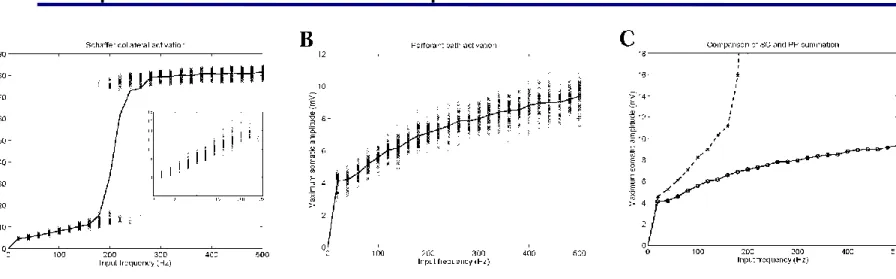
Temporal summation of inputs
Figure: Maximum somatic amplitude as a function of synaptic input frequency (for each simultaneously activated synapse)
Figure A: Synapses are activated through the Schaffer collaterals Figure B: Synapses are activated through the perforant path.
Figure C: Comparison of the SC and PP inputs. Thick line: perforant path inputs, dotted line: Schaffer collateral inputs.
The somatic response to distal dendritic inputs as a function of frequency also saturates below spike threshold.
Integration of PP and SC input is essentially linear
Figure: The amplitude of the somatic response is plotted as we vary both the number of simultaneously activated PP synapses (along the horizontal axis) and the number of SC synapses (also activated simultaneously and 5 ms after the PP input; represented by the different curves, which show results for 120, 100, 80, 60, 40, 20 and 0 SC synapses, respectively, from top to bottom). Crosses indicate individual examples, and curves denote averages.
Integration of PP and SC input is essentially linear
Figure: The amplitude of the average response to the activation of particular numbers of PP and SC synapses is plotted against the sum of the two responses obtained by activating the two pathways separately (crosses). For comparison, the same type of data are shown for summation within SC synapses (the response to the simultaneous activation of two groups of SC synapses vs. the sum of responses to the separate activation of the two groups; indicated by the circles). The inset shows a magnified view of the subthreshold range (the line indicating equality is drawn in for reference).
The modulation of the A-type K ion channel
K(A) can be modulated by several metabotropic neurotransmitter receptors, which shifts the voltage dependence of its activation. This greatly enhances the efficacy of distal inputs in the model. The K(A) channel is active near the resting potential, thus it inhibits the propagation of the depolarization caused by EPSPs. By shifting the activation curve of the K(A) channels to a more positive value this inhibitory effect is reduced.
Figure: Attenuation of signals in the dendritic tree with modulated A-type K channels.
The effect of dendritic Ca
2+spikes
By increasing the density of dendritic Ca(R) channels, dendritic Ca2+
spikes and somatic bursts become possible. This also enhances the potential impact of the perforant path input.
1. Distal dendrite with a dendritic calcium spike at 0.05-0.1 sec.
2. Membrane potential in an intermediate dendrite.
3. Somatic membrane potential.
The effect of dendritic Ca
2+spikes
Figure: Somatic response amplitude as a function of the number of synapses activated.
Calcium spikes (action potentials caused by the opening of voltage-activated channels with permeability to Ca2+) in the dendrites greatly enhance the
propagation efficiency of signals from the distal dendrites, thus the distal inputs have a comparable effect on the somatic membrane potential to the more
proximal inputs.
Integration of excitatory and inhibitory inputs (full bursting model)
Figure: The amplitude of the somatic response is plotted as we vary both the number of simultaneously activated
inhibitory synapses (along the horizontal axis) and the
number of PP inputs
(represented by the different curves, which show results for 1000, 900, …, 200, and 100 PP inputs, respectively, from top to bottom). Crosses indicate individual examples, and curves denote averages.
The model generates action potentials over a threshold, and large enough inhibition prevents somatic depolarization, causing no firing, even in the presence of strong excitatory input.
Simpler neuronal models
• Spiking models: They generate discrete all-or-none impulses. The output is a series of delta functions.
— reduced multicompartmental models (e.g., Pinsky-Rinzel)
— single compartment (e.g., integrate-and-fire, Izhikevich)
• Rate-based models: The output is a continuous firing rate.
• Abstract models (e.g., perceptron, stochastic binary unit)
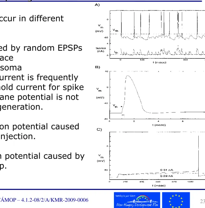
Voltage threshold for action potential generation
Statistical definition of the voltage threshold. A pyramidal cell model was
bombarded for 20 seconds with fast excitatory inputs, and the amplitude of the local maxima of the somatic membrane potential was histogrammed. The peak on the left accounts for the background noise, the middle peak comes from
EPSPs which could not elicit action potentials, and the voltages for right peak are action potentials. The rightmost value of the central hump is the action potential threshold (around -48mV).
Figure: Current-voltage curves in steady state. The somatic membrane potential was clamped and the steady-state current was recorded in pyramidal cells. The instantaneous current I0 (dashed line) was obtained by instantaneously changing the membrane potential from Vrest to Vm. Figure B: detail of Fig. A near the spike threshold. The amplitude of the steady-state current at the peak at -54mV represents the current threshold for spike initiation, and the location of crossing zero Amperes around -47mV represents the voltage threshold for spike generation.
Thresholds – Voltage curves
Thresholds – Spike generation
Spike generation can occur in different ways:
Figure A: Spikes caused by random EPSPs Top: somatic voltage trace
Bottom: current in the soma
Although the somatic current is frequently greater than the threshold current for spike generation, the membrane potential is not high enough for spike generation.
Figure B: A single action potential caused by a 0.2 msec current injection.
Figure C: Single action potential caused by a sustained current step.
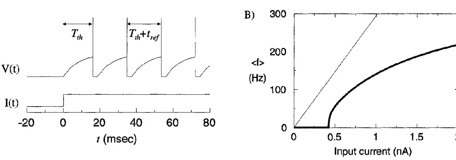
Integrate-and-fire models
Picture: Integrate-and fire models. Incoming inputs charge the capacitor and when the membrane potential reaches Vth, a spike is generated. After a spike, the unit is short-circuited (V=0) for tref duration, preventing spike generation for this time period (absolute refractory period).
Left: Perfect integrate-and-fire unit.
Right: Leaky integrate-and-fire unit. A resistor accounts for the decay of the membrane potential over time.
Integrate-and-fire models: Adapting integrate-and-fire model
An additional conductance is added for modeling firing-rate adaption during spike trains. The ga conductance increases by Ginc after every spike, and decreases exponentially between spikes:
Where is the time constant for decreasing the adaptation conductance.
Integrate-and-fire models
Figure A: Voltage trace of a leaky integrator.
Figure B:
Thick line: Firing rate as a function of the input current in a leaky integrator with refractory period (tref).
Thin line: The f-I curve of a perfect integrator without refractory period is linear.
For a leaky integrate-and-fire model, the time from rest to threshold can be calculated:
The firing rate of integrate-and-fire neurons
The firing rate of a perfect integrator is:
With refractory period:
Where
The firing rate is:
Adapting model vs compartmental model
Figure: Adapting integrate-and-fire unit compared with a biophysically detailed compartmental model (ISI = interspike interval).
Thin solid line: f-I curves of an adapting integrate-and-fire unit.
Thick dashed line: f-I curves of a detailed compartmental model.
The degree of matching between the two models is remarkable,
proving that well-designed simple models can mimic numerous aspects of the behavior of neurons.
Reduced compartmental models
Pinsky-Rinzel model of burst generation in hippocampal CA3 pyramidal cells:
Two-compartment model with burst generation: One soma-like compartment for Na-based action potentials and one dendrite-like compartment for calcium spikes.
Pinsky – Rinzel model for burst generation
The model can produce a wide variety of spiking behaviors
depending on input location, input strength and soma-dendrite
compartment coupling strength.
Left panel: somatic membrane potential.
Right panel: Calcium and slow calcium-dependent
hyperpolarization K channel
(responsible for slowing sustained calcium bursts; denoted by q)
activity curves.
Systematic reduction of compartmental models
Detailed multicompartmental model neurons
+ provide an accurate description of single cell behavior - are too complex to be used in network simulations Abstract model neurons used in network models
- either lack the distinctive features of individual cell types, or - are developed using ad hoc procedures
Goal: to develop a systematic procedure for finding simplified models which provide an optimal approximation of the behavior of complex compartmental model neurons.
(What aspects of behavior? Optimal in what sense?)
Methods
Two-step procedure:
1. Assign the compartments of the full model to clusters which then define the compartmental structure of the reduced model. This assignment also determines the appropriate placement of synapses.
The clusters may also be used in defining the target for the second phase.
2. Optimize the parameters of the reduced model so that some given aspects of its behavior are as close as possible to those of the full model.
Step I: Clustering
• Compartments were characterized by their voltage response to the activation of synapses at various locations — other characterizations (e.g., by the pattern of voltage response in the cell to synaptic activation in the compartment, or by the response to other types of input) are also possible
• The logarithm of the response was used in most cases to enable the algorithms to focus on global patterns
Algorithms used:
K-means clustering (iterative algorithm, maximizes the similarity within clusters and the differences between clusters) with various distance measures (Eucledian, i.e., norm l2, city block, i.e., norm l1, etc.).
Gaussian mixture model, fit using the expectation-maximization (EM) algorithm.
Hierarchical clustering (arranges compartments as the leaves of a binary tree according to pairwise similarity) — results in a series of possible clusterings.
If clustering works right, the geometry of the reduced model also becomes evident
Step II: Parameter Optimization
• Either current injections or synaptic inputs were used for stimulation
• The (arithmetic or geometric) mean responses of compartments of the full model in each cluster were calculated and used as a target for the internal dynamics of the simplified model
• A set of parameters (up to 20) in the reduced model was varied using a parameter search algorithm so that the responses of the reduced model match this average as closely as possible (amplitude, temporal features, or entire waveforms may be matched)
Algorithms used:
• Simulated annealing (with a simplex method implementation) over the "energy landscape" — noisy gradient descent with decreasing
"temperature"
• Genetic algorithm — "evolution" of a population of models
Results I: Clustering
• Clustering revealed a meaningful compartmentalization within the dendritic tree, partly corresponding to functional subregions.
• Different methods and distance measures gave somewhat different results with some conserved features.
• K-means and Gaussian mixture models worked best with logarithmic data
• The optimal number of clusters can be determined if the simulation cost per compartment is known
Figure A: Sum of clustering error and simulation cost at different simulation cost for compartments. Red line: zero simulation cost.
Figure B: Optimal number of compartments as a function of simulation cost.
K-means and Gaussian mixture clustering results
Figures: Clustering results. One horizontal line indicates one
compartment. Same-colored compartments belong to one cluster.
Results II: Parameter Optimization
• Passive characteristics of the reduced cell (dendritic dimensions, RM, CM) and the densities of active conductances (Na, K(A), I(h)) were optimized.
• Non-optimized parameters were set to their average values within the cluster
• We first fit a passive version of the model to the passive version of the full model to provide initial guesses for passive parameters
• The target was either
— (the geometric average of) the amplitude of the voltage response in the corresponding compartments to synaptic stimulation in various compartments
— or the voltage trace in all compartments in response to somatic and dendritic current injections
• Both simulated annealing and the genetic algorithm often found good solutions
• however, in repeated runs, solutions were rather variable, and both algorithms occasionally failed to find a good solution
• simulated annealing appeared to be the most reliable
• when signal attenuation between different parts of the cell was optimized, the behavior of the resulting model was quite similar to that of the original model in several other respects:
— response to step current injection to the soma
— summation of proximal (Schaffer collateral) and distal (perforant path) synaptic inputs
• but failed to reproduce other phenomena such as bursting
•The model could be optimized to reproduce bursting instead.
Results II: Parameter Optimization
Full model vs. Reduced model
(spatial summation in non-bursting models)
Figure A: The morphology of the full model with ~450 compartments.
Figure B: Schaffer collateral and perforant path activation effects on the soma in the full model.
Figure C: Same plots for the reduced model.
Figure D: The morphology of the reduced model consisting of 5 compartments.
Full model vs. Reduced model
(spiking response to somatic current injection)
Figure A: Filled arrows: measurement electrode locations, empty arrow:
current injection location.
Figure B: Membrane potential traces for current injection in the full model.
Figure C: Membrane potential traces for current injection in the reduced model.
Figure D: Voltage measurement electrode locations in the reduced model.
Reduced model, optimal spiking response (simulated annealing)
Figures: Parameter optimization results using the simulated annealing algorithm, with the goal of replicating somatic and dendritic membrane potential traces for the full model. Blue lines indicate traces from the full model, red lines from the reduced model.
Reduced model, optimal spiking response (genetic algorithm)
Figures: Parameter optimization results using a genetic algorithm.
Membrane potential traces for the full and reduced model. Blue lines indicate traces from the full model, red lines from the reduced model.
Summary
In this lesson we learned about:
• Biophysically realistic multicompartmental models: These models describe in detail the morphology of the dendritic tree and every segment (compartment) can contain multiple different ion channels.
• We used a detailed model of a CA1 pyramidal neuron to analyze the propagation and spatial and temporal summation of synaptic inputs.
• We find that the spatial and temporal summation of distal inputs are highly sublinear and saturate, rendering distal inputs almost
ineffective with respect to the somatic membrane potential.
• To enhance distal inputs we modulated A-type K channels and
allowed the generation of dendritic Ca spikes, thus making it possible for distal inputs to cause significant somatic depolarization.
• Next we described simple models for use in network simulations, and listed the pros and cons of such models.
• Finally we introduced methods to systematically reduce complex models to much simpler ones, and demonstrated how we can preserve important features during reduction.
Suggested reading
Books:
•Christof Koch: Biophysics of computation (Oxford University Press), chapter 14
•Jack, J.J.B, Noble, D., Tsien, R: Electric Current Flow in Excitable Cells.
Oxford University Press
•Tuckwell, H.C.: Introduction to Theoretical Neurobiology. Vol 2:
Nonlinear and Stochastic Theories. Cambridge University Press Articles:
•Szabolcs Káli, Tamás F. Freund (2005) Distinct properties of two major excitatory inputs to hippocampal pyramidal cells: a computational
study. European Journal of Neuroscience Vol. 22, pp. 2027-2048 (note:
the parts about the CA1 pyramidal cell model were based on this article)
•Pinsky PF, Rinzel J (1994) Intrinsic and network rhythmogenesis in a reduced Traub model for CA3 neurons. J Comput Neurosci 1:39-60