97
Quasi-Multitask Learning:
an Efficient Surrogate for Constructing Model Ensembles
Norbert Kis-Szab´o1and G´abor Berend1,2
1Institute of Informatics, University of Szeged
2SZTE-MTA Research Group on Artificial Intelligence {ksznorbi,berendg}@inf.u-szeged.hu
Abstract
We propose the technique of quasi-multitask learning (Q-MTL), a simple and easy to imple- ment modification of standard multitask learn- ing, in which the tasks to be modeled are iden- tical. With this easy modification of a standard neural classifier we can get benefits similar to an ensemble of classifiers with a fraction of the resources required. We illustrate it through a series of sequence labeling experiments over a diverse set of languages, that applying Q-MTL consistently increases the generalization abil- ity of the applied models. The proposed ar- chitecture can be regarded as a new regulariza- tion technique that encourages the model to de- velop an internal representation of the problem at hand which is beneficial to multiple output units of the classifier at the same time. Our experiments corroborate that by relying on the proposed algorithm, we can approximate the quality of an ensemble of classifiers at a frac- tion of computational resources required. Ad- ditionally, our results suggest that Q-MTL han- dles the presence of noisy training labels better than ensembles.
1 Introduction
Ensemble methods are frequently used in machine learning applications due to their tendency of in- creasing model performance. While the increase in the prediction performance is undoubtedly an important aspect when we train a model, it should not be forgotten that the increased performance of ensembling comes at the price of training multiple models for solving the same task.
The question that we tackle in this paper is the following:Can we enjoy the benefits of ensemble learning, while avoiding its overhead for training models from scratch multiple times?This question is highly relevant these days, since state-of-the- art neural models tend to be extremely resource- intensive on their own (Strubell et al.,2019), pro-
hibiting their inclusion in a traditional ensemble setting.
Our proposed architecture simultaneously offers the benefit of ensemble learning, while avoiding its drawback of training multiple models. The method introduced here employs a special form of mul- titask learning (MTL). Caruana (Caruana,1997) argues in his seminal work that MTL can be a use- ful source of introducing inductive bias into ma- chine learning models. Standard MTL have been shown to be fruitfully applicable in solving a se- ries of NLP tasks: Collobert and Weston (2008);
Plank et al.(2016);Rei(2017);Kiperwasser and Ballesteros(2018);Sanh et al.(2018),inter alia.
We introduce quasi-multitask learning (Q-MTL), where the goal is to simultaneously learn multi- ple neural models that solveidentical tasks, while relying on ashared representationlayer.
Besides the considerable speedup that comes with the proposed technique, we additionally ar- gue that by applying multiple output units on top of a shared parameter set is beneficial, as we can avoid converging to such degenerate internal repre- sentations that are highly tailored for a particular classification model. In that sense, Q-MTL can also be viewed as an implicit regularizer.
Our experiments with Q-MTL illustrate that the presence of multiple classifier layers for the same task affect each other positively – similar to ensem- ble learning – without the additional overhead of actually training multiple models.
A similar technique have already been de- rived from MTL called Pseudo-Task Augmenta- tion (Meyerson and Miikkulainen, 2018), which builds on the idea of common representation, but the management of these tasks differs. We con- ducted experiments comparing the two methods for a greater comprehension of the differences.
2 Applied models
We release all our source code used for our experiments athttps://github.com/N0rbi/
Quasi-Multitask-Learning/. Our models are based on the sequence classification framework from Plank et al.(2016) implemented in DyNet (Neubig et al., 2017). Figure 1 provides a vi- sual summary of the different architectures we implemented. Figure 1bhighlights that Q-MTL has the benefit of training multiple classification models over the same internal representation, as opposed to traditional ensemble model, which re- quires the training of multiple LSTM parameters as well (cf. Figure1c).
2.1 Baseline architecture
Our baseline classifier is a bidirectional LSTM (Hochreiter and Schmidhuber, 1997) incorporat- ing character and word level embeddings. We first compute the input embedding for the network at positionias
ei=wi⊕ −→ci ⊕ ←c−i,
where⊕is the concatenation operator,widenotes the word embedding,−→ci and←c−i refers to the left-to- right and right-to-left character-based embeddings, respectively. We subsequently feed ei into a bi- LSTM, which determines a hidden representation hi ∈Rmfor every token position ashi =−→hi⊕←h−i, i.e., the concatenation of the hidden states of the two LSTMs processing the input from its beginning to the end, and in reverse direction.
The final output of the network for token position igets computed as
yi=sof tmax(ReLU(hiV+bV)W+bW) (1) with V ∈ Rh×m and bV ∈ Rm denoting the weight matrix and the bias of a regular percep- tron layer withm outputs, whereasW ∈ Rm×c and bW ∈ Rc are the parameters of the neuron performing classification over thectarget classes.
2.2 Q-MTL architecture
The Q-MTL network behaves similarly to the model introduced in Section2.1, with the notable exception that it trainskdistinct classification mod- els, all of which operate over the same hidden repre- sentation as input obtained from a single bi-LSTM unit.
More concretely, we replace the single predic- tion of the standard single task learning (STL)
BiLSTM coffee
Verb ReLU BiLSTM coffee
Verb ReLU BiLSTM coffee
Noun ReLU
(a) Sequence of single task learners (STLs)
Σ
Noun
BiLSTM
Verb ReLU BiLSTM coffee
Noun
ReLU Noun
ReLU
(b) Quasi-Multitask Learning (Q-MTL)
Σ
Noun
BiLSTM coffee
Noun ReLU BiLSTM coffee
Verb ReLU BiLSTM coffee
Noun ReLU
(c) Ensemble
Figure 1: A schematic illustration of the different archi- tectures employed in our experiments. Quasi-Multitask Learning (Q-MTL) averages the predictions of multiple classification units similar to ensembling without the computational bottleneck of adjusting the parameters of multiple LSTM cells.
model from Eq.1 by a series of predictions for Q-MTL according to
yi,j =sof tmax(ReLU(hiV(j)+b(j)V)W(j)+b(j)W), (2) with j ∈ {1, . . . , k}. As argued before, this ap- proach behaves efficiently from a computational point of view, as it relies on a shared representation hifor all thekclassification units.
The loss of the network for token positioniand gold standard class labely∗i can be conveniently generalized as
lQ−M T L(i) =
k
X
j=1
CE(y∗i,yi,j),
whereCE denotes categorical cross entropy loss andkis the number of (identical) tasks in the Q- MTL model, with the special case ofk= 1result- ing in standard STL.
Losses from the different outputs can be effi- ciently aggregated for backpropagation, hence the shared LSTM cell benefit from multiple error sig- nals without the actual need of going through mul- tiple individual forward and backward passes.
Q-MTL outputskpredictions by all of its pre- diction units, however, we can as well derive a combined prediction from the distinct outputs of
Q-MTL according to
1 k
k
X
j=1
sof tmax(ReLU(hiV(j)+b(j)V)W(j)+b(j)W), (3) which is a weighted average according to the pre- dicted probabilities of the distinct models. As in- troducing averaging at the model-level would elim- inate diversity of the individual classifiers (Lee et al.,2015), this kind of averaging took place in a post-hoc manner, only when making predictions.
2.3 Traditional ensemble model
As an additional model, we also employ a tradi- tional ensemble of kindependently trained STL models. We define the prediction of the ensemble model by averaging the predictions ofkindepen- dent models as
1 k
k
X
j=1
sof tmax(ReLU(h(j)i V(j)+b(j)V)W(j)+b(j)W).
(4) The distinctive difference between Eq. 4and the Q-MTL model formulation in Eq.3is that ensem- bling relies on the hidden representations originat- ing fromkindependently trained LSTM models as denoted by the superscripts of the hidden states in h(j)i . Such an ensemble necessarily requires approximatelyk-times as much computational re- sources compared to Q-MTL, due to the LSTM models being trained in total isolation. For the above reason, ensembling is a strictly more expen- sive form of training a model, therefore we regard its performance as a glass ceiling for Q-MTL.
3 Experiments
Our model uses character embeddings of 100 di- mensions and the word representations get initial- ized by the 64-dimensional pre-trained polyglot word embeddings (Al-Rfou et al., 2013) as sug- gested byPlank and Agi´c(2018). We use the bi- LSTM introduced in the previous section. We re- fer to the hidden representation of the LSTM for readability ashi∈R200which stands for the con- catenation of −→
hi,←−
hi ∈ R100. Instead of directly applying a fully-connected layer to perform clas- sification based onhi, we first transformhiby an intermediate perceptron unit with ReLU activation – as shown in2. The perceptron transformshiinto 20 dimensions, that is, we haveV ∈R20×200. Our motivation with the extra non-linearity introduced
by ReLU is to encourage an increased diversity in the behavior of the different output units.
Upon training the LSTMs, we used the default ar- chitectural settings employed byPlank et al.(2016), i.e., we relied on a word dropout rate of 0.25 (Kiper- wasser and Goldberg,2016) and an additive Gaus- sian noise (withσ = 0.2) over the input embed- dings. We trained all our models for 20 epochs using stochastic gradient descent with a batch size of1. First, we assess the quality of Q-MTL towards POS tagging, then we evaluate it on named entity recognition as well.
When comparing the performance of different approaches, Q-MTL models are compared against the average performance ofkSTL models, where kdenotes the number of task in the case of Q-MTL.
ThekSTL models are also used to derive a single prediction by the ensemble model.
3.1 POS tagging experiments
We set our POS tagging related experiments on 10 treebanks from the Universal Dependencies dataset v2.2 (Nivre et al.,2018), namely the Greek- GDT (el), English-LinES (en), Basque-BDT (eu), Finnish-FTB (fi), Croatian-SET (hr), Hungarian- Szeged (hu), Indonesian-GSD (id), Dutch-Alpino (nl), Tamil-TTB (ta) and Turkish-IMST (tr) tree- banks. These treebanks not only cover a typolog- ically diverse set of languages, but they also vary substantially in the number of available training sequences between 400 (for Tamil) and 14980 (for Finnish).
3.1.1 Experiments with the number of tasks We first investigate how changing the value ofk, i.e., the number of simultaneously learned tasks, af- fects the performance of Q-MTL. We experimented withk ∈ {1,10,30}. Based on the results in Ta- ble1, we set the number of tasks to be employed ask= 10for all upcoming experiments. In order to choosekwithout overfitting to the training data, this experiment was conducted on the development set.
3.1.2 Comparing Q-MTL with STL
Following the recommendation in Dodge et al.
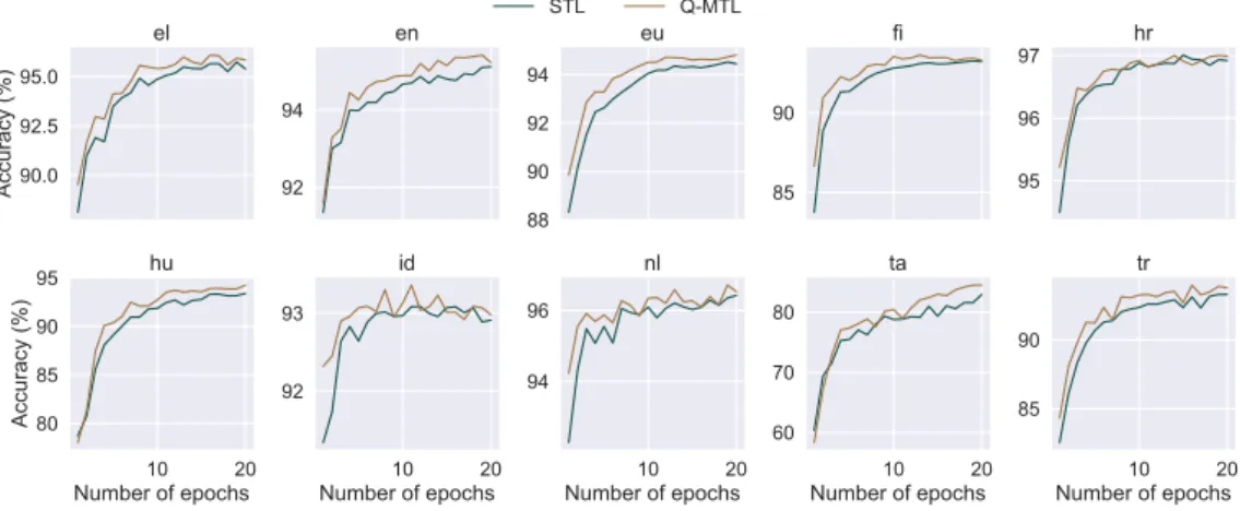
(2019), we report learning curves over the devel- opment set as a function of the number epochs in Figure2As a general observation, we can see that Q-MTL tends to perform consistently better than STL models right from the beginning of training.
$FFXUDF\
HO
HQ
HX
IL
KU
1XPEHURIHSRFKV
$FFXUDF\
KX
1XPEHURIHSRFKV
LG
1XPEHURIHSRFKV
QO
1XPEHURIHSRFKV
WD
1XPEHURIHSRFKV
WU 67/ 407/
Figure 2: The accuracy of the different model types over the training epochs on the dev set.
Table 1: Results of Q-MTL on the dev sets for varying number of tasks employed (k).
k el en eu fi hr hu id nl ta tr Avg.
1 95.61 94.99 94.49 93.19 96.84 93.95 93.05 96.05 82.74 93.61 93.45 10 95.84 95.23 94.81 93.30 96.99 94.25 92.98 96.53 84.48 93.78 93.82 30 95.86 95.21 94.59 93.09 96.93 93.79 93.25 96.27 83.85 93.46 93.63
Directly comparing the classifiers One benefit of Q-MTL is that it learnskdifferent classification models during training with only a marginal com- putational overhead compared to training a STL baseline, since all the tasks share a common inter- nal representation. As discussed earlier, we can combine the predictions from thekclassifiers from Q-MTL according to Eq.2. It is also possible, how- ever, to use thekdistinct predictions of Q-MTL. In what follows next, we compare the performance of thekSTL models we train to thekclassifiers that are incorporated within a Q-MTL model.
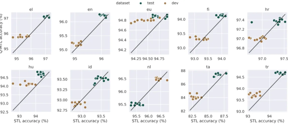
Upon comparing the performance of a Q-MTL classifier with a STL model, we made it sure that the overlapping parameters (matrices V andW) were initialized with the same values and that they receive the training instances in the exact same or- der. This way the performance achieved by theith output of Q-MTL is directly comparable with the ithSTL baseline. Comparison of the results of the individual outputs of Q-MTL and their correspond- ing STL counterpart are included in Figure3.
Training Q-MTL models withktasks simulta- neously is not only faster than trainingkdistinct STL models separately, but the individual Q-MTL models typically outperform their baseline counter- parts evaluated against both the development and the test data.
The regularizing effect of Q-MTL We have ar- gued earlier that Q-MTL has an implicit regular- izing effect. Among most recent techniques, such as dropout (Srivastava et al.,2014), weight decay (Krogh and Hertz,1992) is one of the most typical form of regularization for fostering the general- ization capability of the learned models. When employing weight decay, we add an extra term pe- nalizing the magnitude of the values learned by our model, which results in an overall shrinkage in the values of the model parameters.
Figure4illustrates that the effects of employing Q-MTL is similar to applying weight decay, as the Frobenius norm of the parameter matrices from the classifiers of Q-MTL are substantially smaller than those of the STL classifiers. This observation holds for both the of parameter setsV andW. Recall that the initial values for these matrices were identical for both Q-MTL and STL.
3.1.3 Comparison to an ensemble of classifiers
We next compared the Q-MTL technique with en- semble learning. Our comparison additionally as- sesses the sensitivity of the different approaches to- wards the presence of noisily labeled tokens during training. To do so, we conducted multiple experi- ments for each language, for which we randomly replaced the true class label of a token by some pre-
95 96 97 95
96 97
Q-MTL accuracy (%)
el
95 96
95.0 95.5 96.0
en
94.25 94.50 94.75 94.2
94.4 94.6 94.8
eu
93.0 93.5 94.0 93.0
93.5 94.0
fi
97.0 97.5
96.8 97.0 97.2 97.4
hr
93 94
STL accuracy (%) 92.5
93.0 93.5 94.0 94.5
Q-MTL accuracy (%)
hu
93.0 93.5 STL accuracy (%) 92.75
93.00 93.25 93.50
id
95.5 96.0 96.5 STL accuracy (%) 95.5
96.0 96.5
nl
82.5 85.0 87.5 STL accuracy (%) 82
84 86
88 ta
93 94
STL accuracy (%) 93.0
93.5 94.0 94.5
tr
dataset test dev
Figure 3: Scatter plot comparing the accuracy of the individual classifiers from Q-MTL (k= 10) and their corre- sponding STL counterpart. Each model that is above the diagonal line performs better after training in the Q-MTL setting.
0 25 k.kF
el en eu fi hr
STL Q-MTL 0
25 k.kF
hu
STL Q-MTL id
STL Q-MTL nl
STL Q-MTL ta
STL Q-MTL tr
V W
Figure 4: The average Frobenius norms of the learned parameter matrices V and W for the different ap- proaches and treebanks.
/DEHOQRLVH
$FFXUDF\
$YHUDJH
PHWKRG 67/
407/
HQVHPEOH
Figure 5: Model performances averaged over the 10 treebanks, when a varying amount of noisy training samples are introduced during training.
defined probabilityp ∈ {0,0.1,0.2,0.3}. During the random replacement of the class labels, we en- sured that the same tokens got randomly relabeled by the same label for the different approaches.
Figure5contains the performance of the three different models in conjunction with the different amounts of noisy labels introduced to the training set. We can observe from Figure5that Q-MTL out- performs STL irrespective to the amount of noisy tokens being present encountered during training.
Figure5further reveals that the performances of the ensemble models – which are based on the predic- tions of the STL classifiers – are dominantly better than the average performance of the individual STL models. When mislabeled tokens are not present in the training data at all, ensemble also has a slight advantage over Q-MTL, however, this advantage of the ensembling model gradually fades out as the proportion of noisy training labels increases.
Indeed, for the case when 30% of the training la- bels are randomly replaced, the performance of Q-MTL reaches that of the ensemble model. The proposed approach has the additional benefit over the ensemble model that it requires a fraction of computational resources as we will demonstrate it in Section3.1.5.
3.1.4 Comparison to Pseudo-Task Augmentation
Pseudo-Task Augmentation (PTA) architecture (Meyerson and Miikkulainen,2018) introduces a similar architecture to Q-MTL for leveraging a bet- ter representation of the task by fitting multiple outputs to the same task. PTA makes a series of predictions according to
yi,j =sof tmax(hiW(j)+b(j)W). (5) PTA introduces two special subroutines, named asDecInitandDecUpdate. These subroutines in- troduce various heuristics with the goal of encour- aging the different decoders to behave differently.
DecInit DecInitgets called right before the start of the training and can contain any of the following three methods. PTA-I means that the weight of the
$FFXUDF\
HO
HQ
HX
IL
KU
/DEHOQRLVH
$FFXUDF\
KX
/DEHOQRLVH
LG
/DEHOQRLVH
QO
/DEHOQRLVH
WD
/DEHOQRLVH
WU
/DEHOQRLVH
$YHUDJH
$9*#0/3 %(67#0/3 $9*#0/3 %(67#0/3
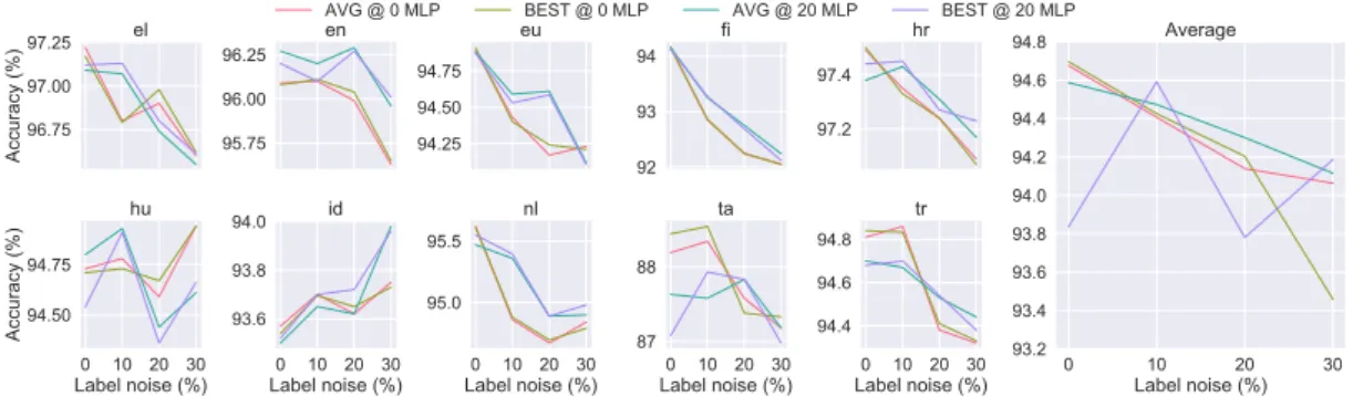
Figure 6: PTA and Q-MTL compared in an analogue manner. The model with the highest dev score (BEST) is compared to model averaging (AVG) and MLP (20 MLP) compared to linear classifier (0 MLP). From PTA (BEST
@ 0 MLP) to Q-MTL (AVG @ 20 MLP) we can see all combinations of these parameters.
tasks get different random initialization. PTA-F, which freezes all ktasks except for the first one.
Finally, PTA-D adds dropout independently to the tasks.
DecUpdate DecUpdateintroduces the so-called meta-iterationinto the learning process. Ameta- iterationis invoked afterMthgradient update. The methods used inDecUpdateall require a ranking of the tasks based on their dev dataset performance.
This makes performing an evaluation step neces- sary at the beginning of eachmeta-iteration. The goal of the ranking is to identify the best task (BT) with the highest dev set performance.
PTA introduces three methods for theDecUp- dateas well. PTA-P perturbs the weight matrix of the tasks excluding theBT. Hyperturb (PTA- H) modifies the tasks in the same manner, but in- stead of adding noise to the weight matrices, noise gets added to the hyperparameters of the tasks (in our case it is the dropout probability preceding the softmax layers). The remaining method is called greedy (PTA-G), which takes the parameters of BT and replaces the actual parameters for all the remainingk−1decoders besidesBT.
The most similar PTA method to Q-MTL is PTA- I, with the main difference that Q-MTL uses an extra transformation and a ReLU non-linearity over the hidden representation of the LSTM (cf. Eq.2 and Eq.5for Q-MTL and PTA-I, respectively).
Another key difference is that PTA uses model selection (BEST), whereas Q-MTL relies on model averaging (AV G). This means that PTA makes prediction for test instances during inference based on the model which achieves best performing dev set accuracy at the end of the training phase. Q- MTL, on the other hand, aggregates all the models according to Eq.3.
Figure6shows the effects of the different com- binations of inference strategies (BEST/AVG) and the usage of a Multi-Layered Perceptron (MLP) in the model (0M LP/20M LP). In these experi- ments the 0 MLP means we do not add the extra layer before the output. Note, that theAV Ginfer- ence strategy used in conjunction with the0M LP architecture is essentially equivalent to the PTA-I architecture.
Figure6 demonstrates that the Q-MTL model with its MLP layer can facilitate the use of model averaging shown in Eq.3as it outperforms the Q- MTL using model selection (BEST @ 20 MLP).
On the other hand it is indeed discouraged to use the AV G model when no MLP is applied, as BEST often outperformsAV Gin case of 0 MLP.
Interestingly, when the train set contains high label noise, the later observation seems to pivot towards the ensemble of linear classifiers. Additionally, we can see that the MLP layer improves the tolerance of the models to the increasing label noise, as it outperforms 7 out of 10 treebanks the model not employing extra ReLU non-linearity.
As an interesting note, the Q-MTL has an im- proved performance for Indonesian as the amount of noisy training labels increases. A possible ex- planation for this is that corrupting the class labels of the training data can be viewed as an alterna- tive form of label smoothing (Szegedy et al.,2016), which is known to increase the generalization abil- ity of neural models.
After the detailed differentiation between PTA-I and Q-MTL we also compare Q-MTL to the more complex PTA variants that were introduced inMey- erson and Miikkulainen (2018). We conducted these experiments for English only because of the computational overhead introduced by the meta-
Table 2: Comparison of Q-MTL to the different types of PTA. This table shows the performance (%) of Q- MTL and the different PTA models on the en POS tag- ging dataset.
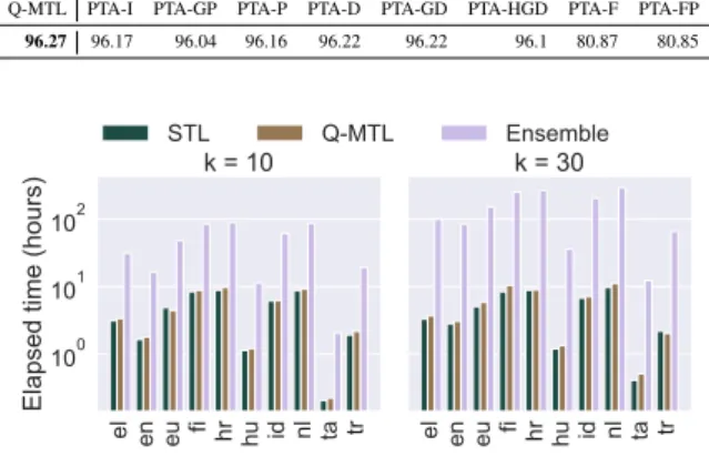
Q-MTL PTA-I PTA-GP PTA-P PTA-D PTA-GD PTA-HGD PTA-F PTA-FP 96.27 96.17 96.04 96.16 96.22 96.22 96.1 80.87 80.85
HO HQ HX IL KU KX LG QO WD WU
(ODSVHGWLPHKRXUV
N
HO HQ HX IL KU KX LG QO WD WU
N 67/ 407/ (QVHPEOH
Figure 7: Training times of the different approaches for the different languages.
iterations being part of the PTA approach. In cases when there are more than one letter after the prefix of the keyword, it refers to a combination of multi- ple approaches (eg. PTA-HGD: hyperturb, greedy, dropout).
Table2shows that while most PTA architectures slightly underperform the Q-MTL, two variants of PTA – namely freeze (F) and freeze combined with perturb (FP) – had a substantially inferior perfor- mance.
These experiments have also shown that the meta-iterations of PTA are responsible for the non- gradient based updates create a considerable com- putational overhead – as noted above – compared to the traditional SGD without external heuristics.
We usedM = 100for our POS tagging classifiers.
This means, that 100 training samples are followed by an evaluation on the dev set, making the training phase 5 and a half hours on average for the different PTA models, while our method took slightly less than 2 hours to finish training. We do not report the performance of all eight methods due to the limitation by this training time overhead.
3.1.5 Comparison of training times
One of the main benefits of Q-MTL resides in its training efficiency compared to traditional en- semble models as also demonstrated by Figure7, which includes the training times for the different approaches. We plot the training times on the loga- rithmic scale for better readability for bothk= 10 andk= 30. We can see that the training times for
STL and Q-MTL practically concur, whereas the overall costs of ensembling exceeds the training time of STL and Q-MTL models by a factor ofk.
The training times reported in Figure 7 were obtained without GPU acceleration – on an Intel Xeon E7-4820 CPU – in order to simulate a set- ting with limited computational resources. We also repeated training on a TITAN Xp GPU. The GPU- based training was 3 to 10 times quicker depending on the languages, but the relative performance be- tween the different approaches remained the same, i.e., STL and Q-MTL training times did not dif- fer substantially, whereas the ensemble model took k-times as much time to be created.
This training overhead is due to the number of excess parameters in the ensemble and Q-MTL models. Given we have ak = 5English model, the ensemble has5times the parameter numbers of STL while the Q-MTL has only1.003times the number of STL parameters.
3.2 Evaluation on Named Entity Recognition We also conducted experiments on the CoNLL 2002/2003 shared task data on named entity recog- nition (NER) in English, Spanish and Dutch (Tjong Kim Sang,2002;Tjong Kim Sang and De Meulder, 2003). For these experiments, we report perfor- mance in terms of overall F1 scores calculated by the official scorer of the shared task. We trained models withk = 10and compared the average performance of the individual STL models to the performance of the Q-MTL and ensemble models.
Table 3a shows the results for NER over the different languages, corroborating our previous ob- servation that Q-MTL is capable of closing the gap between the performance of STL models and the much more resource-intensive ensemble model derived fromkindependent models.
In our POS tagging experiment, we trained models on treebanks of radically differing sizes, whereas during our NER experiments, we had ac- cess to training data sets of comparable sizes (rang- ing between 218K and 273K tokens). In order to simulate the effects of having access to limited training data on NER as well, we artificially relied on only 10% of the available training sets.
These results for the limited training data setting are included in Table3b, from which we can see that Q-MTL manages to preserve more of its origi- nal performance, i.e., 87.5% on average as opposed to the ensemble and STL models, which preserved
Table 3: F1 performance scores for the NER experi- ments.
(a) 100% training data used
Avg. STL Q-MTL Ensemble
en 86.68 86.88 87.86
es 82.28 82.35 83.76
nl 81.84 83.15 83.61
Avg. 83.60 84.13 85.07
(b) 10% training data used
Avg. STL Q-MTL Ensemble
en 77.54 80.24 78.52
es 70.71 71.57 72.56
nl 68.47 69.16 70.33
Avg. 72.42 73.66 73.80
only 86.7% and 86.4% of their original F-scores.
4 Related work
Caruana(1997) showed that neural networks can be trained for multiple tasks, leveraging cross domain information. More recently,Søgaard and Goldberg (2016);Sanh et al.(2018) argues that solving low- level NLP tasks can improve the performance of high level tasks. Additionally,Plank et al.(2016);
Bingel and Søgaard (2017) show that better per- forming models can be trained by introducing mul- tiple auxiliary tasks.Rei(2017) proposes an auxil- iary task for NLP sequence labeling tasks, where the auxiliary tasks is to predict the previous and next word in the sequence. Our results complement these findings by showing that this generalization property holds even if the tasks are the same.
Meyerson and Miikkulainen(2018) introduced Pseudo-Task Augmentation a similar architecture that aims to build a robust internal representation from multiple classifier units optimized for the same task in the same network. Section 3.1.4 describes the similarities and differences to our method. PTA architecture is evaluated on multitask as well, while our work only considers single tasks at the moment.
Ruder and Plank (2018) has shown that self- learning and tri-training can be adapted to deep neural nets in the semi-supervised regime. Their tri-training architecture resembles our approach in that they were utilizing multiple classifier units that
were built on top of a common representation layer for providing labels to previously unlabeled data.
Cross-view training (CVT) (Clark et al.,2018) resembles Q-MTL in that it also employs a shared bi-LSTM layer used by multiple output layers. The main difference between CVT and Q-MTL is that we are utilizing an bi-LSTM to solve the same task multiple times in a supervised setting, whereas Clark et al. used it to solve different tasks in a semi-supervised scenario.
A series of studies have made use of ensemble learning in the context of deep learning (Hansen and Salamon, 1990; Krogh and Vedelsby, 1995;
Lee et al., 2015; Huang et al., 2017). Our pro- posed model is also related to the line of research on mixture of experts proposed by Jacobs et al.
(1991), which has already been applied success- fully in NLP before (Le et al.,2016). The main difference in our proposed architecture is that the internal LSTM representation is shared across the classifiers, hence a more efficient training could be achieved as opposed to training multiple indepen- dent expert models as it was done inShazeer et al.
(2017).
Model distillation (Hinton et al., 2015) is an alternative approach for making computationally demanding models more effective during inference, however, the approach still requires training of a
“cumbersome” model first.
5 Conclusions
We proposed quasi-multitask learning (Q-MTL), which can be viewed as an efficiently trainable al- ternative of traditional ensembles. We additionally demonstrated that it acts as an implicit form of reg- ularization as well. In our experiments, Q-MTL consistently outperformed the single task learning (STL) baseline for both POS tagging and NER. We have also illustrated that Q-MTL generalizes better on smaller and noisy datasets compared to both STL and ensemble models.
The computational overhead for the additional classification units in Q-MTL is infinitesimal due to the effective aggregation of the losses and the shared recurrent unit between the identical tasks.
Although we evaluated Q-MTL over an LSTM, the idea can be applied for more resource-heavy ar- chitectures, like transformer (Vaswani et al.,2017) based models where training an ensemble would be too expensive. This is the future direction of our research.
Acknowledgements
This research was supported by the European Union and co-funded by the European Social Fund through the project ”Integrated program for train- ing new generation of scientists in the fields of computer science” (EFOP-3.6.3-VEKOP-16-2017- 0002) and by the National Research, Development and Innovation Office of Hungary through the Ar- tificial Intelligence National Excellence Program (2018-1.2.1-NKP-2018-00008).
References
Rami Al-Rfou, Bryan Perozzi, and Steven Skiena.
2013. Polyglot: Distributed word representations for multilingual nlp. In Proceedings of the Seven- teenth Conference on Computational Natural Lan- guage Learning, pages 183–192. Association for Computational Linguistics.
Joachim Bingel and Anders Søgaard. 2017. Identify- ing beneficial task relations for multi-task learning in deep neural networks. InProceedings of the 15th Conference of the European Chapter of the Associa- tion for Computational Linguistics: Volume 2, Short Papers, pages 164–169. Association for Computa- tional Linguistics.
Rich Caruana. 1997. Multitask learning. Machine Learning, 28(1):41–75.
Kevin Clark, Minh-Thang Luong, Christopher D. Man- ning, and Quoc Le. 2018. Semi-supervised se- quence modeling with cross-view training. InPro- ceedings of the 2018 Conference on Empirical Meth- ods in Natural Language Processing, pages 1914–
1925. Association for Computational Linguistics.
Ronan Collobert and Jason Weston. 2008. A unified architecture for natural language processing: Deep neural networks with multitask learning. In Pro- ceedings of the 25th International Conference on Machine Learning, ICML ’08, pages 160–167, New York, NY, USA. ACM.
Jesse Dodge, Suchin Gururangan, Dallas Card, Roy Schwartz, and Noah A. Smith. 2019. Show your work: Improved reporting of experimental results.
CoRR, abs/1909.03004.
Lars Kai Hansen and Peter Salamon. 1990. Neural network ensembles. IEEE Transactions on Pattern Analysis & Machine Intelligence, (10):993–1001.
Geoffrey Hinton, Oriol Vinyals, and Jeffrey Dean.
2015. Distilling the knowledge in a neural network.
In NIPS Deep Learning and Representation Learn- ing Workshop.
Sepp Hochreiter and J¨urgen Schmidhuber. 1997. Long short-term memory. Neural computation, 9:1735–
80.
Gao Huang, Yixuan Li, Geoff Pleiss, Zhuang Liu, John E. Hopcroft, and Kilian Q. Weinberger. 2017.
Snapshot ensembles: Train 1, get M for free. CoRR, abs/1704.00109.
Robert A. Jacobs, Michael I. Jordan, Steven J. Nowlan, and Geoffrey E. Hinton. 1991. Adaptive mixtures of local experts.Neural Comput., 3(1):79–87.
Eliyahu Kiperwasser and Miguel Ballesteros. 2018.
Scheduled multi-task learning: From syntax to trans- lation. Transactions of the Association for Computa- tional Linguistics, 6:225–240.
Eliyahu Kiperwasser and Yoav Goldberg. 2016. Sim- ple and accurate dependency parsing using bidirec- tional lstm feature representations. Transactions of the Association for Computational Linguistics, 4:313–327.
Anders Krogh and John A. Hertz. 1992. A simple weight decay can improve generalization. In J. E.
Moody, S. J. Hanson, and R. P. Lippmann, editors, Advances in Neural Information Processing Systems 4, pages 950–957. Morgan-Kaufmann.
Anders Krogh and Jesper Vedelsby. 1995. Neural net- work ensembles, cross validation, and active learn- ing. InAdvances in neural information processing systems, pages 231–238.
Phong Le, Marc Dymetman, and Jean-Michel Ren- ders. 2016. Lstm-based mixture-of-experts for knowledge-aware dialogues. InProceedings of the 1st Workshop on Representation Learning for NLP, pages 94–99. Association for Computational Lin- guistics.
Stefan Lee, Senthil Purushwalkam, Michael Cogswell, David J. Crandall, and Dhruv Batra. 2015. Why M heads are better than one: Training a diverse ensem- ble of deep networks.CoRR, abs/1511.06314.
Elliot Meyerson and Risto Miikkulainen. 2018.
Pseudo-task augmentation: From deep multitask learning to intratask sharing—and back.
Graham Neubig, Chris Dyer, Yoav Goldberg, Austin Matthews, Waleed Ammar, Antonios Anastasopou- los, Miguel Ballesteros, David Chiang, Daniel Cloth- iaux, Trevor Cohn, Kevin Duh, Manaal Faruqui, Cynthia Gan, Dan Garrette, Yangfeng Ji, Lingpeng Kong, Adhiguna Kuncoro, Gaurav Kumar, Chai- tanya Malaviya, Paul Michel, Yusuke Oda, Matthew Richardson, Naomi Saphra, Swabha Swayamdipta, and Pengcheng Yin. 2017. Dynet: The dy- namic neural network toolkit. arXiv preprint arXiv:1701.03980.
Joakim Nivre, Mitchell Abrams, and et al. 2018. Uni- versal dependencies 2.2. LINDAT/CLARIN digi- tal library at the Institute of Formal and Applied Linguistics ( ´UFAL), Faculty of Mathematics and Physics, Charles University.
Barbara Plank and ˇZeljko Agi´c. 2018. Distant super- vision from disparate sources for low-resource part- of-speech tagging. InProceedings of the 2018 Con- ference on Empirical Methods in Natural Language Processing, pages 614–620. Association for Compu- tational Linguistics.
Barbara Plank, Anders Søgaard, and Yoav Goldberg.
2016.Multilingual part-of-speech tagging with bidi- rectional long short-term memory models and auxil- iary loss. InProceedings of the 54th Annual Meet- ing of the Association for Computational Linguistics (Volume 2: Short Papers), pages 412–418. Associa- tion for Computational Linguistics.
Marek Rei. 2017. Semi-supervised multitask learn- ing for sequence labeling. In Proceedings of the 55th Annual Meeting of the Association for Compu- tational Linguistics (Volume 1: Long Papers), pages 2121–2130. Association for Computational Linguis- tics.
Sebastian Ruder and Barbara Plank. 2018.Strong base- lines for neural semi-supervised learning under do- main shift. InProceedings of the 56th Annual Meet- ing of the Association for Computational Linguistics (Volume 1: Long Papers), pages 1044–1054. Associ- ation for Computational Linguistics.
Victor Sanh, Thomas Wolf, and Sebastian Ruder. 2018.
A hierarchical multi-task approach for learning em- beddings from semantic tasks.
Noam Shazeer, Azalia Mirhoseini, Krzysztof Maziarz, Andy Davis, Quoc Le, Geoffrey Hinton, and Jeff Dean. 2017. Outrageously large neural networks:
The sparsely-gated mixture-of-experts layer.
Anders Søgaard and Yoav Goldberg. 2016. Deep multi- task learning with low level tasks supervised at lower layers. In Proceedings of the 54th Annual Meet- ing of the Association for Computational Linguistics (Volume 2: Short Papers), pages 231–235. Associa- tion for Computational Linguistics.
Nitish Srivastava, Geoffrey Hinton, Alex Krizhevsky, Ilya Sutskever, and Ruslan Salakhutdinov. 2014.
Dropout: A simple way to prevent neural networks from overfitting. Journal of Machine Learning Re- search, 15:1929–1958.
Emma Strubell, Ananya Ganesh, and Andrew McCal- lum. 2019. Energy and policy considerations for deep learning in NLP. InProceedings of the 57th Annual Meeting of the Association for Computa- tional Linguistics, pages 3645–3650, Florence, Italy.
Association for Computational Linguistics.
Christian Szegedy, Vincent Vanhoucke, Sergey Ioffe, Jonathon Shlens, and Zbigniew Wojna. 2016. Re- thinking the inception architecture for computer vi- sion. InCVPR, pages 2818–2826. IEEE Computer Society.
Erik F. Tjong Kim Sang. 2002. Introduction to the CoNLL-2002 shared task: Language-independent named entity recognition. InProceedings of CoNLL- 2002, pages 155–158. Taipei, Taiwan.
Erik F. Tjong Kim Sang and Fien De Meulder.
2003. Introduction to the CoNLL-2003 shared task:
Language-independent named entity recognition. In Proceedings of the Seventh Conference on Natural Language Learning at HLT-NAACL 2003 - Volume 4, CONLL ’03, pages 142–147, Stroudsburg, PA, USA.
Association for Computational Linguistics.
Ashish Vaswani, Noam Shazeer, Niki Parmar, Jakob Uszkoreit, Llion Jones, Aidan N. Gomez, Lukasz Kaiser, and Illia Polosukhin. 2017. Attention is all you need.CoRR, abs/1706.03762.