Theory of Computing

(1)

Theory of Computing

Tamás Herendi

(2)

Theory of Computing

Tamás Herendi Publication date 2014.

(3)

List of Figures

3.1. Figure 1 ... 9

3.2. Figure 2. ... 10

3.3. Figure 3 ... 10

4.1. The model of Turing machine ... 17

4.2. Parity bit addition to the input word ... 21

4.3. Initial configuration: ... 21

4.4. ... 21

4.5. ... 21

4.6. ... 21

4.7. ... 21

4.8. ... 21

4.9. ... 22

4.10. ... 22

4.11. ... 22

4.12. ... 22

4.13. ... 22

4.14. ... 22

4.15. ... 22

4.16. ... 22

4.17. The computation of the Turing machine on the input word ... 22

4.18. Parity check ... 23

4.19. Initial configuration: ... 23

4.20. ... 24

4.21. ... 24

4.22. ... 24

4.23. ... 24

4.24. ... 24

4.25. ... 24

4.26. ... 24

4.27. ... 24

4.28. ... 24

4.29. ... 25

4.30. ... 25

4.31. ... 25

4.32. ... 25

4.33. ... 25

4.34. ... 25

4.35. The computation of the Turing machine on the input word ... 25

4.36. The composition of and ... 30

4.37. Conditional composition of , and ... 32

4.38. Iteration of ... 34

4.39. Multi tape Turing machine ... 36

(5)

4.40. Simulation of a two-tape Turing machine ... 40

(6)

List of Examples

3.1. Example 1. ... 9 3.2. Example 2. ... 9 3.3. Example 3 ... 10

(7)

Chapter 1. Preface

The present note is based on and made for the Theory of Computing course held at the University of Debrecen.

The the fundamental aim of the course - and therefore of the lecture note - to give an adequate background knowledge for the students of the basics in computability and complexity theory.

The structure of the book is the following:

Chapter 2 describes the necessary concepts and results in formal language theory, related to the general algorithmic problems and definition of the Turing machine.

Chapter 3 contains definitions and properties on the order of growth of functions which are frequently appears in complexity theory.

Chapter 4 discusses the definitions and the related basic properties of Turing machines. The computation of Turing machines, the Church-Turing thesis, the composition of Turing machines and the definition of multi-tape Turing machines and simulation theorems are described here.

In Chapter 5 one can read about the theory of computability, where recursivity, recursively enumerability and their relations are observed. At the end of the chapter some decidability problems are discussed.

Chapter 6 provides definitions and fundamentals on the properties of non-deterministic Turing machines and deals with their Turing equivalence.

In Chapter 7 the time, space and program complexity, the complexity classes defined by them and their relationship are regarded.

Chapter 8 discusses the results related to the class . Among others the witness theorem and - completeness are detailed.

(8)

Chapter 2. Formal languages

As in the case of programs such algorithms are typically created for solving not a particular task, but a group of tasks. The input, output and other related objects - e.g. the algorithm itself - should be defined and used in some general way. To do this we need some basic concepts and results in the theory of formal languages.

We start with some definitions related to functions.

Definition 2.1.

Let and be two arbitrary non-empty sets.

The Cartesian product of the two sets is the set containing pairs from the base sets.

If , then we may use the notation .

Let . The set is called a relation defined on . If for some and we have , then we say that

and are in relation by .

Let be a relation. If and the property implies , then is called

a (partial) function and is denoted by . If , then we use the traditional notation .

If such that , then it is called a total function.

Let be a total function. If such that , then is called a surjective function.

If implies , then is called an

injektive or one-to-one function.

If is both surjective and injective then it is called bijektive.

Remark 2.2.

The traditional notation for the relation is , as we are used with e.g. the relations and .

If and are two function, then the union of them can be defined as the union of relations. This, however, is not necessarily a function. If we assume, that , then is

a function and .

Since in the following parts we want to prove that the mathematical concept of algorithm we construct can be precisely specified, thus the detailed definition of the alphabet, word and language are necessary. There is a particular need to find place of the empty symbol in the structure.

Definition 2.3.

The finite, non-empty set is called an alphabet.

The elements of are called letters (somtemies characters or symbols).

If , then we assume for that . (The symbol is called the empty character.)

(9)

Definition 2.4.

Let be a nonepty set and let be a map.

Assume that

1. ;

2. sympols such that ;

3. and implies if

and only if and ;

4. and ,

such that ;

5. (Induction) Let a statement on the elements of .

If , holds and implies ,

then holds, too;

6. If , then .

Then is called the set of finite words over the alphabet and is called the empty word.

As it is usual, we will use the notation and .

Remark 2.5.

1. Let . The map can be viewed as a transformation, which extends the word by the symbol .

2. One can define a natural embedding between and ,

by .

Thus the elements of can be regarded as finite sequences of elements of .

3. By 6. of Definition 2.4 , which means that and are different, but they are corresponding to each other in the two sets.

4. By 6. of Definition 2.4 the 3. can be extended to the cases és .

5. The 5. pf Definition 2.4 means that every word can be created from the empty word by adding symbols to it.

Thus, if , where ,

then we may denote the word by its traditional notation

.

6. By point 3. the above represenatation is unique.

7. The previous statement can be extended to the empty symbol with

the property .

Definition 2.6.

Let be a function with properties:

1. ;

2. , and .

Then is called the length of the word .

(10)

Formal languages

Theorem 2.7.

the length is well defined.

Proof

By definition, the length of a word means the number of steps the map applied on the empty word to get . Since number and the order of the extension steps are fixed for the creation of , the length is unique. ✓ Remark 2.8.

If a word is regarded as a finite sequence of symbols, then the length is equal to the number of symbols in it.

Definition 2.9.

Let be a binary operation on , i.e. ⋅: with the properties:

1. let ;

2. and implies .

Then the operation is called the concatenation.

Traditionally we use the simpler notation instead of .

The operation of concatenation has the following property.

Theorem 2.10.

if and ,

then .

Proof

The proof is by induction on .

a.) By definition, if , then , which means that the statement holds.

b.) Assume that for a given for all words if , then the statement holds.

Let be a word of length . If the is the last letter of , then for some , where .

By the inductive assumption . Applying the definition of the concatenation,

which means that the statement holds for , too.

Form a.) and b.) by induction the theorem follows. ✓ Theorem 2.11.

(11)

with the binary operation of concatenation is a monoid (semigroup with a unit element).

Proof

The proof is again by induction.

1. The concatenation is associative:

a.)By definition .

b.) Assume, that for a given for all words , if , then the associativity holds. Let

is such that . Then and satisfying and . By the inductive

assumption, for all words the equality holds. Hence

,

which means that the statement is true for , too.

From a.) and b.) by induction the associativity follows.

2. is a unit element.

By definition for all .

The equality can be proven by induction.

a.) By the definition .

b.) Assume for all that if , then . Let be a word of length . Then and , such that and . By the inductive assumption

,

which means that the statement holds for , too.

From a.) and b.) by induction follows.

With this, the proof is complete. ✓ Theorem 2.12.

The operation of concatenation satisfies the simplification rule, i.e.

the eqality implies . Similarly, the equality implies . Proof

(12)

Formal languages

As before, the proof can be done by induction. In the firs case the induction is on , while in then second case the induction is on and , simultaneously. ✓

The following definitions are useful for the description of the structure of word.

Definition 2.13.

Let be such that .

Then is called a prefix, while is called a postfix of . Remark 2.14.

A word is a so called trivial pre- and postfix of itself.

The empty word is a trivial pre- and postfix of any word.

One may define transformations in the form on the set of finite words. These transformation can have some good properties. Some of the most important ones are given in the following.

A transformation is called length preserving,

if the equality holds.

Remark 2.16.

Length preserving transformation e.g. the mirror image, permutation of characters, cyclic permutation, e.t.c.

A transformation is called prefix preserving,

if words , such that .

Remark 2.18.

In the examples of Remark 2.16, the mirror image and cyclic permutation is not, but the character permutation is prefix preserving transformation.

Prefix preserving, but not length preserving, however, the following transformation:

. (Repetition.)

Using the concept of words, we arrive to the definition of an important object of the theory of algorithms.

Let be a finite alphabet. The set is called a (formal) language over .

It is natural idea to define the usual set operations on languages. E.g. if, are two languages, then and are languages, too. The language is called the complement of .

Other important operations on languages are the following.

(13)

Let be two languages. The language is called the concatenation of the languages and denoted by .

Remark 2.21.

Concatenating by itself, we may use the following simplified notation

és , ha .

Let be a language. The language is called the iteration - or the closure for the concatenation - of .

Remark 2.23.

The name closure comes from the fact, that is exactly the smallest language, such that

is a subset of it and closed under concatenation.

Let be a class of languages.

Then the class .

Here denites the complement of . Remark 2.25.

The class is in general not the complement of . Actually is not necessarily empty.

If e.g. is the class of all languages,

then .

Theorem 2.26.

Let and be two class of languages over the same alphabet.

Then

1. ;

2. ;

3. ;

4. if and omly if .

Proof

We apply the usual set theoretic proofs for equalities.

1.We may write the following chain of equivalences

or or .

2. Similarly, we may write the following chain of equivalences:

(14)

Formal languages

and and .

3. In this case we may write:

.

4. By definition if and only if and if and only if . Again by definition if and only if implies . This, however, stands exactly when implies . ✓

(15)

Chapter 3. Order of growth rate

In latter chapters - in particular at complexity observations - one needs the possibility to express the growth rate order (i.e. the asymptotic behaviour) of functions in a unified way. We define a relation for this, with which one can extract the most important, the steepest growing component of functions.

Definition 3.1.

Let be a monotone increasing function.

The set

is called the class of functions, in the order of growth of . If , we say that " is a big O " function.

Remark 3.2.

To make the definition clear, the the best if we assume that is a monotone increasing function.

However, it is not necessary. If we don't do so, many of the observations would became unexpectedly complicate.

Instead of the notation , often the traditional is used.

The most obvious example for the definition if a function bounds an other by above. But this is not necessary to be so. In the following we will demonstrate through some particular example what does the growth rate expresses at first view.

Example 3.1. Example 1.

Assume that . Then the conditions of the definition are fulfilled with the choice , .

Figure 3.1. Figure 1

Example 3.2. Example 2.

(16)

Order of growth rate

Assume that , if . We don' care the relation of the functions for small 's.

Figure 3.2. Figure 2.

Example 3.3. Example 3

Assume , but the function multiplied by a constant is not below .

Figure 3.3. Figure 3

Properties 3.3.

1. (reflexivity)

2. for all .

3. Let and . Then (transitivity)

Proof

(17)

1. Let and . Since for all , thus for all .

2. Let and .Then , i.e. , for all . ✓

3. Let and such that , if and assume that with and the relation

holds if . Then with the choice and , we get ,

if and , i.e. .

Remark 3.4.

1. A transitivity exresses our expectations that if a function grows faster than , then it grows faster than any other, which has slower growth than .

2. The definition of the order of growth rate, can be extended to nonmonotone functions, but

this case is not really important for our purposes.

3. The relation of growth rates are neither symmetric, nor antisymmetric.

A counterexample for the symmetry

( ) is the pair and ,

while a counterexample for the antisymmetry

( ) is the pair and

.

Further properties 3.5.

4. Let and .

Then .

5. Let and .

Then .

6. Let be a monotone increasing function,

whith and .

Then .

Proof

3. Assume that with , , and the relations and are

true. Let and let . Then

.

4. Similarly as before, assume that with , , and the relations and

are true. Let and . Then

.

5. Assume that and are such that holds. Without loss of generality, we may assume

further, that . Since the function is strictly increasing, thus

. Since ,thus .

(18)

Let . By the monotonicity of we have and

✓ Corollaries 3.6.

1. Let .

Then if and only if .

2. Let .

Then if and only if . 3. Let k > 0.

Then and .

4. Let .

Then .

Proof

Corollaries 1, 2, 3 and 4 can be derived from Properties 4, 5 and 6 by simple considerations. ✓ In the following we give the definition of a sequence and a related extremely fast growing function.

Definition 3.7.

Let , be a sequence

of functions with the recurrence relation 1.

2.

3.

The first few members of the sequence are the well known mathematical operations.

1. is the successor, 2. is the addition, i.e.

3. is the multiplication, i.e.

4. is the exponentiation, i.e.

.

The above definition is actually the extension of the usual ones:

1. is defined by the consecutive incrementation of by , times;

2. the multiplication is defined by the consecutive addition of by itself times;

3. the exponentiation is the consecutive multiplication of by itself times, etc..

(19)

With this construction, we obtain a sequence of faster and faster growing functions. By this sequence we can define a function, which grows faster than any of its member:

.

One can, however, define a function, closely related to the above, without the given sequence.

Definition 3.8.

Ackermann function:

Let be a function with the following relation:

1.

2.

3.

The function is called the Ackermann function.

The function is approximately the same as (but somewhat less than it). The firs few values of are the following:

, where k is a number with decimal digits.

Clearly, this value exceeds all imaginable or even exactly describable limits. (It is much more, than the number atomic particles in the universe, by our best knowledge.) And the function grows faster and faster.

To express the order of growth more precisely, other concepts are used, too. Some of them with results on their properties are given below.

Definition 3.9.

Let be a (monotone increasing) function. The set

is called the class of functions in the order of growth of .

Properties 3.10.

1. Let be two functions.

Then if and only if . 2. Let be two functions.

Then if and only if and Proof

1. Let and such that , for all and let and . Then, by

the first inequality,

(20)

, for all ha and by the second inequality

, for all . By definition, this is the same as in the statement of the theorem.

2. By the relations and one find that , , and such that

, if and , if .

Let and . The two inequalities above implies , if

. ✓

Let be a function. The set

is called the class of functions with order of growth less than .

If , we say that " is a small o ".

Properties 3.12.

1. Let be two function.

Then if and oxly if

.

2. Let be a function.

Then .

3. Let be a function.

Then .

Proof

1. Let the constants and be such that , if . Then , if , i.e. for

arbitrary small there exists a bound such that for all greater than the inequality holds. By the definition of limits, this means that . Conversely, means that such that for all . Hence, by a multiplication by we get the statement of our objective.

2. By the definitions, clear that and . Let .

Hence, and such that , if and such that if

.

(21)

Let . With this the inequality holds, for all , which is exactly the statement we wanted to proof.

3. Indirectly, assume that . Then .

With this we find that and such that if and such that

, if .

Let . With this we have and , if , which is a

contradiction. ✓

(22)

Chapter 4. Turing machines

Everyone, who has some relation with informatics has an idea about the concept of algorithms. In the most case we can decide whether the thing under observation is an algorithm or not. At leas in the everyday case. Many of the people think on a computer program in connection with an algorithm, not without any reason. It is not clear, however, if a medical treatment or the walking are algorithms..

If we try to make the concept more exact, we reach some limitations. We have the following obvious expectations:

The algorithm should solve a well defined task or group of tasks.

The algorithm should stand of separable steps and the number of (different) steps are finite.

We want the solution in limited time.

Every step of the algorithm should be well defined.

The algorithm need some input data for determining the particular task of the group of tasks.

The amount of data should be finite, in any sense.

The algorithm should reply to the input. The answer should be finite and reasonable.

Clearly, if one wants to determine the concept of algorithm in a general manner, then some points will be not properly defined. The most critical part is the concept of "step". What does it mean "well defined"? If we give a precise definition, we would reduce our possibilities.

The precise determination of the concept of algorithms are was a subject of many mathematician in the first half of the last century. As a result, many different approach of the subject have arised, e.g. functions, recursive functions, Markov algorithm and Turing machine. Since these are well defined models, we have the feeling that they cannot be completely suitable for the substitution of the concept of the algorithm.

One can prove that the above models are equivalent, which means that every task which can be solved in one of the models, can be solved in all the others.

For the replacement of the concept of algorithm there are still no more general model than the listed ones. In the present lecture notes we will focus on the model of the Turing machine, since this is one of the most clear, easy to understand and expressive enough. Even if it is not so suitable for modeling the modern computer architectures.

With the help of Turing machines one can easily express the concept of computability, i.e. the algorithmic solvability and a precise measure can be introduced for describing the complexity of algorithms and problems.

If one wants to define with mathematical tools the concept of algorithms, the class of possible tasks should be reduced. One should exclude the mechanical operations on physical objects. This does not mean that, physical problems cannot be solved by some algorithmic way, but one have to model it first with some mathematical representation and then the result can be applied to the original problem through some interface.

We assume that the task and its parameters and input data can be represented in a finite way. Accordingly, we will give the input of an algorithm as a finite word over a finite alphabet and we expect the answer in the same way. Thus an algorithm can be regarded as a transformation, which maps words to words. Some of the algorithms have no reply on some input. These represents, so called, partial functions. One can find algorithms, which have only finitely many different answer on their infinitely many different inputs. These are the typical acceptor or decision machines.

Definition 4.1.

Let be an alphabet, be a language, be a word and be a transformation.

We will call algorithmic task (or simple task) the following:

(23)

1. Determine if the relation holds!

2. Determine the value of !

The first kind of tasks are called decision problems, while the second are called transformation problems.

Later we will see that the above easy looking decision problem in general is not easy at all. We will prove that there are problems such that one cannot even decide whether they are solvable or not.

Figure 4.1. The model of Turing machine

1. The definition of the Turing machine

Definition 4.2.

The five tuple is called Turing machine, if : is a finite nonempty set; set of states

: is a finite set with at least elements and ; tape alphabet

; initial state

, nonempty set; final states

; transition function

The above formal definition needs a proper translation. One may think of the following "physical" model.

The Turing machine has three main parts:

1. a tape, infinite in both direction, divided into equal sized cells, containing symbols from the alphabet ; the tape may contain only finitely many characters different from and they should be consecutive;

2. a register, containing values from , which determines the actual behaviour of the Turing machine;

3. a read-write head, pointing always to a particular cell, this connects a tape and the register.

One step of the Turing machine stands of reading the cell under the read-write head and depending on its value, executes some operation, determined by :

- writes back a symbol to the cell under the read-write head and changes it state or - moves the read-write head to the neighbor cells and changes it state.

(24)

Turing machines

Usually the alternative definitions of the Turing machine sets the movement and write in the same step, but separating them makes some definitions much simpler.

The above semantics needs, however, a mathematically well defined "operation".

Definition 4.3.

A configuration of the Turing machine is the four tuple

(= state of the regiser + tape content together with the position of the read-write head)

Remark 4.4.

A Turing machine has a configuration in the form

if or .

Definition 4.5.

We say that the Turing machine reach the configuration from in one step - or directly - (notation ), if

and exactly one of the following holds:

1) , where , and .d

--- overwrite operation

2) , where , and .

--- right movement operation

3) , where , and .

--- left movement operation Remark 4.6.

1. Since is uniquely defined for all and , thus for all proper configuration either there exists a uniquely given direct accessible configuration or there are no any at all.

2. By the definition of the configuration and the remark

after the definition if and ,

then the Turing machine can execute a further step,

if or .

3. By the properties of the symbol , if and , then in the transition the

configuration .

Similarly, if and , then in

the transition the configuration . Definition 4.7.

A computation of a Turing machine is a sequence of configurations such that

1. , where ;

2. , if there exists a directly reachable configuration from (and because of uniqueness,

(25)

it is );

3. , if there are no directly reachable configuration from .

The word is called the input of .

If is such that , then

we say that the computation is finite and the Turing machine terminates in the final state . Then the word is called the output of . Notation: .

If for a word the Turing machine has an infinite computation, then it has no output.

Notation: . (Do not mix it up with the output .)

Remark 4.8.

A Turing machine may have infinite computation on an input word in two ways:

1. there exist a directly reachable configuration ; 2. such that from there are no directly reachable configuration and the state corresponding to is not a final state. (The Turing machine is "frozen" in the configuration .)

2. Acceptor Turing machines

Definition 4.9.

Let be a Turing machine,

and . Then is called an acceptor Turing machine and the states of are called accepting states.

Let be an acceptor Turing machine and let be the accepting states of .

We say that accepts the word , if the computation of on is finite and at termination the Turing machine is in a state from .

Let be an acceptor Turing machine.

Then is

called the language recognized by . Lemma 4.12.

(26)

Turing machines

Let be an acceptor Turing machine and let . Then transformator Turing machine such that

if and only if . Proof

The new Turing machine can be defined using . The states of and the transition function can be redefined on the way, that the Turing machine does not finish the computation there, but erase the tape and writes a 1 instead. ✓

The above Lemma implies that acceptor Turing machines basically do not differ from transformation Turing machines. They computes the characteristic function of the recognised language.

3. Representation of Turing machines

The specification of a Turing machine means to give a description of five tuple in the general definition. For the objects and it is not a great adventure but for the transition function requires a bit more efforts. Since it is a function defined on a finite domain with values from a finite set, fortunately there are no big difficulties to manage.

The different representations are explained on two particular Turing machines.

The first Turing machine executes a parity bit encoding on words over the alphabet . This is a typical transformation task. Prefix preserving, but not length preserving mapping. The essence of the encoding is that one have to count the number of symbol 's in the input word and extend it by a new symbol such that the number of 's in the output should be even. This transformation is one of the most simple but most efficient, widely applied error detection encoding.

Examples: (Parity bit addition)

In: Out:

At the real life application equal word length is assumed, but here we simply don't care about this restriction.

The second Turing machine checks whether the input word satisfies the parity property or not, i.e. if there are even number of 's in it. If the answer is yes, then we accept the word, if no, then we reject it.

3.1. Look up table representation:

With look up table representation, the transition function can be given in several ways. In one of them the columns of the table are related to the different states, while the rows are related to the possible input symbols, read by the read-write head. The values in the table are the function values at the corresponding arguments.

If the transition function is not everywhere defined (partial function), the table contains gaps.

Example: Parity bit addition

One possible solution for the task is the following Turing machine:

where ,

, and

:

(27)

Figure 4.2. Parity bit addition to the input word

Here is the final state, is the initial state and in the same time it has the notion, that the processed part contains even number of 's. Furthermore, has the notion, that the processed part contains odd number of 's.

The states and are for moving the read-write head and remembering to the parity.

The Turing machine executes the following computation on a given input:

In:

Figure 4.3. Initial configuration:

Figure 4.4.

Figure 4.5.

Figure 4.6.

Figure 4.7.

Figure 4.8.

(28)

Turing machines

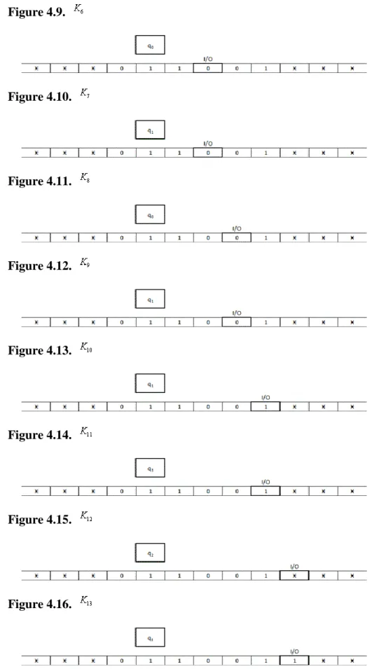
Figure 4.9.

Figure 4.10.

Figure 4.11.

Figure 4.12.

Figure 4.13.

Figure 4.14.

Figure 4.15.

Figure 4.16.

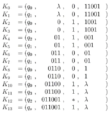
One may recognize, that the description of a computation in the above way is rather uncomfortable, but expressive. Describing the configurations in the form of their definition is much more efficient.

Figure 4.17. The computation of the Turing machine on the input word

(29)

Example: Parity check

One possible solution for the task is the following Turing machine:

where ,

, and :

Figure 4.18. Parity check

Here is an accepting, while is a rejecting state, i.e. and . Furthermore, is the initial state and in the same time it has the notion, that the processed part contains even number of 's. The state has the notion, that the processed part contains odd number of 's and the states and are for moving the read-write head and remembering to the parity.

The Turing machine executes the following computation on a given input:

In:

Figure 4.19. Initial configuration:

(30)

Turing machines

Figure 4.20.

Figure 4.21.

Figure 4.22.

Figure 4.23.

Figure 4.24.

Figure 4.25.

Figure 4.26.

Figure 4.27.

Figure 4.28.

(31)

Figure 4.29.

Figure 4.30.

Figure 4.31.

Figure 4.32.

Figure 4.33.

Figure 4.34.

The description of the computation by the configurations in the form of their definition:

Figure 4.35. The computation of the Turing machine on the input word

(32)

Turing machines

3.2. Graph representation:

3.3. Representing Turing machines by enumeration:

The transition function can be given by the enumeration of its values on its possible arguments.

The transition function of Turing machine for parity bit generation:

(33)

The transition function of Turing machine for parity check:

3.4. Examples

1. Turing machine for mirroring the input word: . 2. Turing machine for mirroring the input word:: .

3. Turing machine which increase the input word - regarded as a binary number: , where .

3.5. Problems

1. Give the description of a Turing machine, which writes the word to its tape!

(34)

Turing machines

2. Give the description of a Turing machine, which writes the word to its tape!

3. Give the description of a Turing machine, which inverts its input word, i.e. exchanges every to a and every to a !

4. Give the description of a Turing machine, which swaps the symbols pairwise of the input word!

e.g..

5. Give the description of a Turing machine, for deciding which symbols are more frequent in the input word! If there are more 's, then it terminates in the state , if there are more 's, then it terminates in the state and if the are equal then it terminates in the state .

4. Church-Turing thesis

As we have discussed at the beginning of the chapter, an algorithm can be regarded as a function on words. The input word is called the task and the output word is called the solution.

By the definitions above, Turing machines represents similar functions.

The question arises naturally, which tasks can be solved by a Turing machine. The following statement approaches this question.

Church-Turing thesis 4.13.

Let be an algorithm transforming words to words,

i.e. .

Then there exists a Turing machine such

that .

Remark 4.14.

1. If does not terminate on a given input , then is undefined and hence we should assume that does not terminate, too.

2. The Church-Turing thesis can be applied both on the transformationa and decision tasks.

In the latter case the output of the algorithm is not a word, but a decision. (e.g. yes or no.)

Observing the Church-Turing thesis one may find that the concept of algorithms has no mathematical definition.

It implies that the statement has no mathematical proof, although it has a truth value. It is rather unusual, but only disproof may exist - if the thesis is wrong. To do this, it is enough to find a task, which can be solved by some method - regarded as an algorithm - and can be proven to be unsolvable by a Turing machine.

The first appearance of the thesis is around the years 1930. Since then, there are no disproof, although many people tried to find one. A standard method for this, is to define a new algorithm model and try to find a task which can be solved by it, but not with a Turing machine. However, until now, all model was proven to be not stronger than the model of the Turing machine. If the class of solvable tasks for the observed model is the same as in the case of Turing machines, it is called Turing equivalent.

Some of the most well known Turing equivalent algorithm models:

(35)

• calculus

• RAM machine

• Markov algorithm

• Recursive functions

• Cellular automaton

• Neural network model

• Genetic algorithms

5. Composition of Turing machines

In many cases the Turing machine solution for a given task is not obvious. One may define, however, some general operation on Turing machines, with which more complex Turing machines can be constructed from simpler ones. Using these operations many of the proofs became easier. It extends the possibilities to apply our standard approach for programming, while the mathematical accuracy is preserved.

Definition (composition of Turing machines) 4.15.

Let and

be two Turing machines and assume that .

The Turing machine (or ) is defined by the following:

, where , , ,

and . Here

where

, for all and , and

for all and .

Remark 4.16.

The union of the functions is defined on the way given in Chapter 2 as the union of relations.

Theorem 4.17.

The Turing machine defined above has

the property ,

i.e. can be regarded as the consecutive execution of and .

Proof

(36)

Turing machines

Let be a word of arbitrary length .

The computation of on the input word is , while the computation of on the input word

is .

If terminates on the input word , let and the let computation of on the input word be .

By definition, since , thus .

Again, by definition, if , then , i.e. while we have .

Hence, if does not terminate on , then does not terminate, neither.

If , where , then terminates. In this case , i.e. the content of its tape is .

By definition, continues computing according to , i.e. it goes to the configuration and then it moves the read-write head back to the beginning if the tape. When it reaches the first symbol, it transits to the configuration - here -, but this is equal to the configuration . Since , if , thus for the next steps, i.e., if does not terminate on , then does not terminate, neither.

Otherwise .

Figure 4.36. The composition of and

✓

Using acceptor Turing machines, the conditional execution can be defined, too.

Definition (conditional execution) 4.18.

Let ,

and be three Turing machines.

Assume that

, , ,

and .

We define the Turing machine

by the following:

, where

(37)

, ,

,

and . Here

, where

for all and , for all and , for all and furthermore

, where .

Remark 4.19.

Multiple conditional execution can be

defined by splitting to more than 2 parts and assigning to each part a new Turing machine.

Theorem 4.20.

Let and and denote the answer of by , if it terminates in a state from

on the input and denote the answer by , if it terminates in a state from on the input .

The above defined Turing machine has:

, if the answer of on the input word is or

, if the answer of on the input word is .

Proof

Let be a word of arbitrary length . The computation of on the input word is , while the computation of

on the input word is . If terminates on , let and the computation of on is , while the computation of on is .

Again by definition, if , then , i.e. while , we have .

Hence, if does not terminate on , then does not terminate, too.

(38)

Turing machines

If , where , then terminates. In this case , i.e. the content of the tape is .

By definition, continues computing according to .

a.) If , then first it goes to the configuration and then it moves the read-write head back to the beginning if the tape. When it reaches the first symbol, it transits to the configuration

- here -, but this is equal to the configuration .

Since , if , thus for the next steps, i.e., if does not terminate on , then does not terminate, neither.

Otherwise

b.) If , then first it goes to the configuration and then it moves the read-write head back to the beginning if the tape. When it reaches the first symbol, it transits to the configuration

- here - , but this is equal to the configuration .

Since , if , thus , for the next steps, i.e., if does not terminate on , then does not terminate, neither.

Otherwise .

Figure 4.37. Conditional composition of , and

✓

If one would like to execute a Turing machine repeatedly in a given number of times, then a slight modification of the definition is required, since we assumed that the set of states of the Turing machines to compose are disjoint.

Definition (fixed iteration loop) 4.21.

Let be a Turing machine.

The Turing machine is

defined such that the corresponding components of is replaced by a proper one with a sign.

With this notation let

(39)

. In general:

Let and , if . Remark 4.22.

By Theorem 4.17. .

Iteratively applying, we have , where the depth of embedding is .

(The notation of is just the same as it is usual at composition of functions.)

The Turing machine denoted by can be regarded as the consecutive execution of repeated times.

There is one tool missing already from the usual programming possibilities, the conditional (infinite) loop.

Definition (iteration) 4.23.

Let and

, .

The Turing machine

is defined by:

, where ,

, ,

and . Here , where

for all and , , and

. Remark 4.24.

If , then does not terminate on any input (= infinite loop).

Theorem 4.25.

,

i.e. can be regarded as the iterative execution of .

Proof

(40)

Turing machines

Let be a word of arbitrary length .

The computation of on the input word is , while the computation of on the input word

is .

If terminates on the input word .

Again, by definition, if , then , i.e. while we have By this, if does not terminate on , then does not terminate, neither.

If , where , then terminates. In this case , i.e. the content of its tape is .

By definition, if continues computing according to , if it terminates.

If , then it goes to the configuration and then it moves the read-write head back to the beginning if the tape. When it reaches the first symbol, it transits to the configuration - here -, but this is equal to the initial configuration of with the input word .

Then , i.e. it behaves as it would start on the input .

Figure 4.38. Iteration of

✓

Remark 4.26.

One may eliminate the returning of the read-write head to the beginning of the tape. Then the execution of the next Turing machine continues at the tape position where the previous one has finished its computation. In most of the cases this definition is more suitable, but then it would not behave as the usual function composition.

Using these composition rules, we may construct more complex Turing machines from simpler ones.

(41)

Some of the simpler Turing machines can be the following:

• moves the read-write head position to the right

• observes cell on the tape, the answer is "yes" or "no"

• moves the read-write head to the first or last position of the tape

• writes a fixed symbol to the tape

• copies the content of cell to the next (left or right) cell

• ...

Composite Turing machines

• writes a symbol behind or before the input word

• deletes a symbol from the end or the beginning of the input word

• duplicates the input word

• mirrors the input word

• decide whether the length of the input word is even or odd

• compares the length of two input words

• exchanges representation between different number systems

• sums two words (= numbers) Example

Let be the set of possible input words and let the following Turing machines be given:

1. : observes the symbol under the read-write head; if it is a ,then the answer is "yes" otherwise the answer is "no"

4. : moves the read-write head one to the left 5. : moves the read-write head one to the right 6. : writes a symbol on the tape

7. : writes a symbol on the tape 8. : writes a symbol on the tape

Applying composition operations, construct a Turing machine which duplicates the input word, i.e. it maps to

!

First we create a Turing machine for moving the read-write head to the rightmost position:

(42)

Turing machines

.

The leftmost movement can be solved similarly:

The Turing machine which search for the first to the right is the following:

.

The Turing machine which search for the first to the left is the following:

.

6. Multi tape Turing machines, simulation

One can introduce the concept of multi tape Turing machine as the generalisation of the previous model. Here the state register of the Turing machine has connection with more than one tape and every tapes has its own independent read-write head.

Figure 4.39. Multi tape Turing machine

Definition (multi tape Turing machine) 4.27.

Let be an integer. The tuple is called a -tape Turing machine, if ha

is a finite, nonempty set; set of states is a finite, nonempty set; ; tape alphabet

; initial state

, nonempty; final states

; transition function

Similarly to the simple (single tape) Turing machines, one may define the concept of configuration, step and computation.

(43)

Let be -tape Turing machine and .

is called the set of possible configurations of , while its elements are called the possible configurations of .

Then is the set of possible description of one tape of .

Let be a -tape Turing machine and let be two configurations of it.

Assume that

where , ,

, and

, where . We say that the Turing machine

reach the configuration from in

one step - or directly - (notation ), if for all exactly one of the following holds:

1) and

, where .

--- overwrite operation

2) ,

and

.

--- right movement operation

3) ,

and

.

--- left movement operation Remark 4.30.

The multitape Turnig machines execute operations independently - but determined together by its transition function - on its tapes.

Let be a -tape Turing machine.

A computation of the Turing machine on the input word of length

is a sequence of

configurations such that

1. , where and

, if ;

(44)

Turing machines

2. , if there exists a directly reachable configuration from (and because of uniqueness, it is );

3. , if there are no directly reachable configuration from .

If is such that ,

then we say that the computation is finite and the Turing machine terminates in the final state .

If , then the word

is called the output of . Notation: .

If for a word the Turing machine has an infinite computation, then it has no output.

Notation: . (Do not mix it up with the output .)

Remark 4.32.

It is assumed in the definition of the multitape Turing machines, that the input and output are on the first tape.

This is a general convention, but of course in particular cases the input or output tapes can be elsewhere.

Obviously, the multi tape Turing machine model is at least as strong as the original, single tape model, since every single tape Turing machine can be extended by arbitrary number of tapes, which are not used during computations. These single and multi tape Turing machines are identical from operational point of view.

To observe the strength of the different models, we need a precise definition to describe the relation of models.

Let and be two Turing machines.

We say that simulates , if

and the equality holds.

Remark 4.34.

By Definition 4.34., arbitrary input of is a possible input of , too.

Furthermore, means that if terminates on the input word and it computes the output word , then terminates and

gives the output , too. If does not terminate on the input , then not terminate, neither.

It is possible, that can compute many more,

(45)

than , but it can reproduce the computation of .

Theorem 4.35.

Let be a -tape Turing machine.

Then there exist a -tape Turing machine, which simulates .

Proof

The complete proof would yield the elaboration of many technical details, thus only a rough proof is explained.

The proof is constructive, which means that define a suitable Turing machine here and prove that it is the right one.

The basic idea of simulation is that we execute the steps of the original Turing machine step by step.

For this purpose, the simulating Turing machine continuously stores the simulated one's actual configurations.

In general, one may observe, that a Turing machine can store information in two ways: by the states and on the tapes. Since there are only finitely many states and the number of configurations are infinite, it is natural to store the necessary data on the tape. Since the simulating Turing machine has only a single tape, thus all information should be stored there. There are many possibilities to do so, but we will choose the one, which divides the tape into tracks and uses them to store the tapes and position of the read-write heads of the original Turing machine. In this case the symbols of the new Turing machine are -component vectors of the original symbols extended by a - component vector of 's for the positions of read-write heads.

The definition of then:

Let be the Turing machine which simulates , where

and

is the transition function, described below:

As it is explained at the beginning of the proof, we will store on the tape of all information of the original Turing machine. In the meantime the state of stores among others, the actual state of .

Initially, we will assign the configuration of for the configuration of by the following way:

The components of are ,

, where if and , or otherwise, furthermore

(46)

Turing machines

, where (i.e. the length of is longer by one, than the longest word on the tapes of ),

for all , where (if , then let ) and

, if or otherwise (i.e. the read-write head is over the th position of tape ), for all

and .

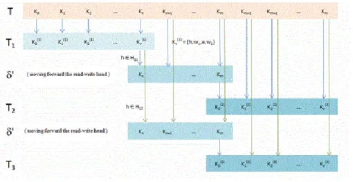
In a particular -tape case it looks like:

Figure 4.40. Simulation of a two-tape Turing machine

The Turing machine executes the following computational phases from an above given initial state:

Phase 1. Reading

Scan the tape and where it finds at a read-write position, the corresponding symbol is stored in the corresponding component of the state.

In the example above, until the fourth step, is unchanged. Afterward, it takes the value . After the fifth step it changes again to the value .

If it read the last nonempty cell on the tape, it steps to the next phase.

In the example, the state of does not change further in this phase, since there are no more read-write head stored on the tape.

Phase 2. The execution of the step .

In this phase it does only one thing: if , then it goes to the state ,

where

Actually, it computes and stores in its state the simulated Turing machine's transition (state change, tape write and movement).

Then it continues with phase tree.

Phase 3. Writing back.

Theory of Computing

Theory of Computing

Tamás Herendi

Theory of Computing

Table of Contents

List of Figures

List of Examples

Chapter 1. Preface

Chapter 2. Formal languages

Chapter 3. Order of growth rate

Example 3.1. Example 1.

Figure 3.1. Figure 1

Example 3.2. Example 2.

Figure 3.2. Figure 2.

Example 3.3. Example 3

Figure 3.3. Figure 3

Chapter 4. Turing machines

Figure 4.1. The model of Turing machine

1. The definition of the Turing machine

2. Acceptor Turing machines

3. Representation of Turing machines

3.1. Look up table representation:

Figure 4.2. Parity bit addition to the input word

Figure 4.3. Initial configuration:

Figure 4.4.

Figure 4.5.

Figure 4.6.

Figure 4.7.

Figure 4.8.

Figure 4.9.

Figure 4.10.

Figure 4.11.

Figure 4.12.

Figure 4.13.

Figure 4.14.

Figure 4.15.

Figure 4.16.

Figure 4.17. The computation of the Turing machine on the input word

Figure 4.18. Parity check

Figure 4.19. Initial configuration:

Figure 4.20.

Figure 4.21.

Figure 4.22.

Figure 4.23.

Figure 4.24.

Figure 4.25.

Figure 4.26.

Figure 4.27.

Figure 4.28.

Figure 4.29.

Figure 4.30.

Figure 4.31.

Figure 4.32.

Figure 4.33.

Figure 4.34.

Figure 4.35. The computation of the Turing machine on the input word

3.2. Graph representation:

3.3. Representing Turing machines by enumeration:

3.4. Examples

3.5. Problems

4. Church-Turing thesis

5. Composition of Turing machines

Figure 4.36. The composition of and

Figure 4.37. Conditional composition of , and

Figure 4.38. Iteration of

6. Multi tape Turing machines, simulation

Figure 4.39. Multi tape Turing machine

Figure 4.40. Simulation of a two-tape Turing machine