ApparentconvergenceofPad´eapproximantsforthecrossoverlineinfinitedensityQCD PHYSICALREVIEWD 103, 034511(2021)

(1)

Apparent convergence of Pad´e approximants for the crossover line in finite density QCD

Attila Pásztor ,^1,*Zsolt Sz´ep ,^2,† and Gergely Markó ^3,‡

1ELTE Eötvös Loránd University, Institute for Theoretical Physics, Pázmány P. s. 1/A, H-1117 Budapest, Hungary

2MTA-ELTE Theoretical Physics Research Group, Pázmány P. s. 1/A, H-1117 Budapest, Hungary

3Fakultät für Physik, Universität Bielefeld, D-33615 Bielefeld, Germany

(Received 1 October 2020; accepted 19 January 2021; published 25 February 2021) We propose a novel Bayesian method to analytically continue observables to real baryochemical potentialμBin finite density QCD. Taylor coefficients atμB¼0and data at imaginary chemical potential μÎBare treated on equal footing. We consider two different constructions for the Padé approximants, the classical multipoint Padé approximation and a mixed approximation that is a slight generalization of a recent idea in Padé approximation theory. Approximants with spurious poles are excluded from the analysis. As an application, we perform a joint analysis of the available continuum extrapolated lattice data for both pseudocritical temperature T_c at μÎB from the Wuppertal-Budapest Collaboration and Taylor coefficientsκ2andκ4from the HotQCD Collaboration. An apparent convergence of½p=pand½p=pþ1 sequences of rational functions is observed with increasing p. We present our extrapolation up to μB≈600MeV.

DOI:10.1103/PhysRevD.103.034511

I. INTRODUCTION

Despite considerable effort invested so far, the phase diagram of QCD in the temperature(T)-baryon chemical potential(μB) plane still awaits determination from first principles. At the moment, the only solid information available is the curvature of the crossover temperature [1–3], together with some upper bound on the absolute value of the next Taylor coefficient of order Oðμ⁴_BÞ [2,3].

These results come either from the evaluation of Taylor coefficients with lattice simulations performed atμB ¼0or via simulations performed at imaginaryμB, where the sign problem is absent, with the Taylor coefficients obtained from a subsequent fit.

Whether the input data are the Taylor coefficients or the values of a function at several values of the imaginary chemical potential, fact is that the numerical analytic continuation needed to extrapolate the crossover to real μBis a mathematically ill-posed problem[4,5]. This means that although the analytic continuation of a function

sampled inside some domain D is uniquely determined by the approximant used, the extension of a function differing on D by no matter how small an amount can lead to arbitrarily different values at points outsideD. That is to say: analytic continuation is unique, but is not a continuous function of the data. For such ill-posed prob- lems, the only way to achieve convergence in the results is to use some kind of regularization. This makes sure that the noise in the data is not overemphasized by the analytic continuation. As the noise is reduced, the regularizing term is made weaker. This leads to a kind of double limit when the regularization and the noise are taken to zero together.

The simplest kind of regularization for analytic continuation is the use of some ansatz, which is assumed to describe the physics both in the range where data is available, and in the range where one tries to extrapolate.

The conservative view is to use for analytic continuation few-parameter approximants, which all fit the data well, and perform the continuation only in a range where they do not deviate much from each other, assessing the systematic error of the continuation from this deviation. Here we pursue a more adventurous approach, by considering a sequence of approximants of increasing functional com- plexity, and trying to observe whether they converge or not.

In the absence of physically motivated ansatz, a good guess is to study the½p=p(diagonal) and½p=pþ1(subdiagonal) Pad´e sequences, as these are only slightly more complicated to work with than polynomials, but have far superior convergence properties. Ordinary Pad´e approximants

*apasztor@bodri.elte.hu

†szepzs@achilles.elte.hu

‡gmarko@physik.uni-bielefeld.de

Published by the American Physical Society under the terms of the Creative Commons Attribution 4.0 International license.

Further distribution of this work must maintain attribution to the author(s) and the published article’s title, journal citation, and DOI. Funded by SCOAP³.

(2)

(i.e., rational functions constructed using approximation- through-order conditions to match the Taylor expansion of a function at a given point) are known to converge uniformly on the entire cut plane for functions of Stieltjes type[6](which have a cut on the negative real axis). For this class of functions the subdiagonal sequence of multipoint (or N-point) Pad´e approximants [7], also know as the Schlessinger point method in the context of scattering theory [8], is also convergent (see[9]and references therein). For a meromor- phic function, on the other hand, Pad´e approximants are known to converge in measure[10,11], i.e., almost every- where on the complex plane, in stark contrast to polynomial approximations, which stop converging at the first pole of such a function.

While the convergence properties of Pad´e approximants in exact arithmetic are often very good, even in cases where the mathematical reason for the convergence is not fully understood yet, these approximations tend to be very fragile in the presence of noise. This often manifests itself in spurious poles, whose residue goes to zero as the noise level is decreased, as well as spurious zero-pole pairs (called Froissart doublets[12]). The distance between the zero and the pole goes to zero as the noise decreases, eventually leading to the annihilation disappearance of the doublet. There is a large body of mathematical literature devoted to the removal of these spurious poles. Procedures which do so typically involve some further regularization, like in Ref. [13], where this is based on singular value decomposition, or monitoring the existence of Froissart doublets for later removal, like in Ref.[14]. In cases where the noise level on the data cannot be arbitrarily decreased,¹ the exclusion of spurious poles is mandatory if one wants to go to higher order approximants in the analysis.

When dealing with numerical analytic continuation, we need to select the approximant from a class of possible functions (i.e., a model) and a method to take into account the data (i.e., a fitting method). For the former we use two types of rational approximants, the classical multipoint Pad´e approximants recently used for analytic continuation in Refs. [15–17] and a slight generalization of the Pad´e- type approximant introduced and studied recently in[18].

The parameters of the multipoint Padé approximant are determined solely in terms of the interpolating points and information on Taylor coefficients, if it exists, can be taken into account in the second, data fitting step. In contrast, the Padé-type approximant allows for a joint use of interpolating points and Taylor coefficients in determining the parameters of the approximant. Although the focus in [18] was on the diagonal sequence ½p=p of Padé-type approximants, the method can be easily generalized to

construct the subdiagonal sequence as well. For the data fitting step we use a Bayesian analysis. The likelihood function ensures that approximants are close to both the data on the Taylor coefficients atμB¼0 and the data at purely imaginary μB, while a Bayesian prior makes sure that spurious poles are excluded from the extrapolation.

Considering two different types of Pad´e approximants is a nontrivial consistency check, mainly because the exact form of the prior distribution will be different for the two cases, as the number of interpolation point where the function values will be restricted is different.

We note that while Bayesian methods—especially var- iations of the maximum entropy method with different entropy functionals—for the analytical continuation to real time are quite commonly used in lattice QCD[19–26], as far as we are aware, such methods have not been applied to the analytic continuation problem inμB so far. The only related example we are aware of is Ref. [27], where a Bayesian method is used to extract high order derivatives of the pressure aroundμB¼0from data at imaginaryμB. One must note however, that the mathematical problem in that paper is that of numerical differentiation, which is distinct from the analytic continuation problem discussed here.

This paper, therefore, is the first attempt of using this class of mathematical techniques to the analytic continuation problem in finite density QCD.

The above mentioned fragility of the Padé approximation method when applied to noisy data is the main reason that most of the previous applications to finite density QCD employ low order approximants. Padé approximants were used in this context to analytically continue to real values of μBthe pseudocritical temperature values obtained at imaginary chemical potential for various number of flavors and colors[28–31]. The convergence of a Padé sequence was seemingly not in the focus of these investigations, with the exception of[28]. A related problem in finite density QCD, where Padé approximants have also been considered, is the calculation of the equation of state at finite chemical potential. An early work that uses a high order Taylor expansion in an effective model is Ref.[32]. Two recent examples in lattice QCD are Refs.[33,34]. The low order Padé approximants used in the above studies are not yet expected to take advantage of the superior convergence properties of the Padé series. This is in sharp contrast to the case in statistical physics, where in Ising-like models the Taylor coefficients are known exactly to high orders[35– 37]. However, even a low order Padé approximant represents a resummation of the Taylor series, which is exploited when applied outside the radius of convergence of the Taylor series. The main advantage of the Bayesian approach presented here is the ability to go to considerably higher orders, at the cost of what we believe are physically reasonable extra assumptions.

The paper is organized as follows. In Sec.IIwe introduce the mathematic tools used for our analysis. First we treat the

1E.g., if the noise is only coming from machine precision in floating point arithmetic, the Froissart doublets can often be removed by simply using multiple precision arithmetic for the

“naive” algorithm.

(3)

novel Pad´e-type approximants in the absence of noise.

Since the traditional multipoint Padé approximants are quite well known, they are relegated to AppendixA. Next, we discuss the Bayesian analysis in the presence of noise in a general manner that includes both the multipoint Padé and the mixed Padé approximant case. In Sec. III we turn to physical applications. We first demonstrate the effective- ness of Padé approximants in a chiral effective model.

Finally, we perform a joint analysis of the continuum extrapolated lattice data on the Taylor coefficients atμB¼0 and the crossover line at imaginary μB. Appendix B summarizes the formulas relating our notational conven- tions on the Taylor coefficients to those found elsewhere in the literature.

II. NUMERICAL METHOD FOR ANALYTIC CONTINUATION

A. Pad´e-type rational approximants in the absence of noise

Using the notation of[18]the mathematical formulation of analytic continuation is as follows. Assuming the existence of a continuous real function f∶R→R, we would like to know its value for t >0given that:

(i) at a number of interpolating points τi<0, i¼ 1;…; l, the valuesf_i≔fðτiÞare known,

(ii) a number of coefficientsc_i,i¼0;…; kin the Taylor expansion

fðtÞ ¼c₀þc₁tþ þc_kt^k ð1Þ around t¼0 are known.

A widely used method to tackle the problem is to fit a rational fraction²

½n=m≡Rⁿ_mðtÞ≡N_nðtÞ D_mðtÞ≔

P_n

i¼0a_itⁱ P_m

i¼0b_itⁱ; ð2Þ to the set of function values and/or available derivatives.

When only derivatives at t¼0are used, one obtains the ordinary Pad´e approximant in which the coefficients of both the denominator and the numerator are fully determined by the Taylor coefficients by imposing the approximation-through-order conditions³ Rⁿ_mðtÞ ¼fðtÞþ Oðt^mþnþ1Þ. This condition implies that the Taylor expansion of the Pad´e approximant aroundt¼0agrees with the Taylor expansion of the function up to and including the order of the highest Taylor coefficient known.

When only the set of function values at the interpolating points are used, one obtains the so-calledmultipoint Pad´e

approximant, which is particularly useful in numerics in its continuous fraction formulation because the coefficients can be determined easily from recursion relations. For odd number of points N¼2kþ1, k≥0, one obtains the approximant ½k=k, while for even number of points N¼2k, k≥1, one obtains the approximant ½kþ1=k.

More details can be found in Appendix A, where the construction of the multipoint approximant C_N is summarized.

As mentioned in Ref. [38] (see p. 16), an obvious modification of the multipoint Pad´e approximation can be given if any number of successive derivatives exists at the points where the value of the function is known.

Recently such a modification, called Pad´e-type rational approximantwithn¼m¼kwas constructed in[18], with k being the degree up to (and including) which the expansion of the approximant matches the Taylor expansion of the function. The denominator of this ½k=k approximant is fixed by function values at arbitrarily chosen interpolating points and the coefficients of the numerator are obtained by imposing the approximation- through-order conditions.

It is easy to generalize the construction used in [18]to obtain Pad´e-type approximants for whichl≠k. Withkþ1 coefficients of the Taylor expansion (including the value of the function at zero) one can construct many Pad´e-type approximants of this type, one just has to satisfy the relation nþm¼kþl. In this case kþ1 coefficients of the numeratorN_nðtÞ are determined from the approximation- through-order conditions, meaning that strictly speaking Rⁿ_m satisfies by constructionn≥k, and the remainingnþ m−k¼l coefficients are fixed by function values at l number of interpolating points via f_iD_mðτiÞ ¼N_nðτiÞ;

i¼1;…; l.

In what follows we shall use Pad´e-type approximants of the formR^p_p andR^p_pþ1, with p≥1, satisfying2p¼kþl and2pþ1¼kþl, respectively. To construct for example R³₄ðtÞusingc₀,c₁, andc₂, one equates(1)with(2)and after cross multiplication one matches the coefficients oft⁰,t¹, and t². This gives a₀¼c₀, a₁¼c₁þb₁c₀, and a₂¼ c₂þb₁c₁þb₂c₀, which are common for all approximants withn≥2. Using these expressions for a₀, a₁, and a₂ in N₃ðtÞ, one sees that the five conditions f_iD₄ðτiÞ ¼ N₃ðτiÞ; i¼1;…;5represents a system of linear equations for the five unknowna₃,b₁,b₂,b₃,b₄, which can be easily solved numerically with some standard linear algebra algorithm. As for theR¹₂ðtÞapproximant, this is constructed very similarly to the original Pad´e approximant, only the condition on the third derivative (unknown in our case) is replaced byR¹₂ðτ₁Þ ¼f₁, whereτ₁is an interpolating point.

B. Bayesian approach

The Bayesian approach [39] that considers the data sample fixed and the model parameters as random variables

2One can choose b₀¼1 without loss of generality, having nþmþ1 independent coefficients.

3One equates the expansion offðtÞwithRⁿ_mðtÞ, cross multiply and then equates the coefficients of t on both sides of the equation.

(4)

gives a perspective on the curve fitting problem which is particularly suited for a meta-analysis of data with noise.

We do not include Pad´e approximants of different order in one large meta-analysis, rather we perform a separate Bayesian analysis of the different order approximants, in order to study their convergence properties as the order of the approximation is increased. For an½n=mPad´e approximant, the model parameters are the coefficients a⃗ ¼ ða₀; a₁;…; a_nÞand⃗b¼ ðb₁; b₂;…; b_mÞ, with a total ofnþ mþ1 coefficients to be determined. The posterior prob- ability can be written as:

Pð⃗a;bjdataÞ ¼⃗ 1

ZPðdataja;⃗ ⃗bÞP_priorð⃗a;bÞ;⃗ ð3Þ where assuming Gaussian errors around the correct model parameters, the likelihood is given by:

Pðdataja;⃗ bÞ ¼⃗ exp

−1 2χ²

; χ²¼χ²_Taylorþχ²_Imμ_B;

χ²_Taylor¼X^T

i¼1

c_i−^∂ⁱ^Rⁿ^m_∂ðμ^ðμ2^B^;⃗a;^bÞ^⃗ BÞⁱ j_μ_B_¼0

₂ σ²ci

;

χ²_Imμ_B ¼X^L

j¼1

f_j−Rⁿ_mðiμ^I_B;j;a;⃗ bÞ⃗ ₂

σ²_f_j ; ð4Þ

withT being the number of derivatives known at μB¼0 and L being the number of function values known for μ²_B <0. Z is a normalization constant. The Taylor coefficients atμB¼0 are clearly correlated, but their correla- tion matrix was not given in Ref. [2] so we ignore the correlations. If the correlations between the Taylor coefficients are known, including them in our method is completely straightforward. The data at different values of imaginaryμBcome from different Monte Carlo runs, and are thus uncorrelated.

The variables that the Bayesian analysis code uses for the construction of the Padé approximants are not the coefficients of the polynomial themselves. For the multipoint Padé approximants we use a number of interpolated values at fixed node points inμˆ²B≔μ²B=T². For the case of Padé- type approximants we use a smaller number of interpolated values at node points and a number of derivatives at μB ¼0. These are of course in a one-to-one correspon- dence with the polynomial coefficients, once the restriction b₀¼1 has been made in Eq. (2). Details of the implementation will be discussed in Sec.III B.

An important part of our procedure is that we do not work with the space of all Pad´e approximants of order

½n=m, rather, the allowed approximants are restricted by the prior, which always contains a factor that excludes

spurious poles both in the interpolated and the extrapolated range. Due to this factor of the prior, the method is only applicable when no physical poles are expected in the aforementioned ranges.

The prior also contains a further factor—the exact form of which for the two different Pad´e approximants will be discussed in Sec.III B—which prevents extra oscillations of the interpolants in the μ²B<0 range, which are not warranted by the data. This is enforced by using a prior distribution of the interpolated values at the node points at fixedμ²_B=T²range. We have checked that our results are not sensitive to the choice of the node points. This is also expected on mathematical grounds, since unlike polynomial interpolants, rational interpolants are not extremely sensitive to the choice of the node points used for the interpolation[40].

Putting all the above information together, the prior can be given as an implicit condition on the model parametersa⃗ andb⃗ in the following form

Ppriorða;⃗ bÞ⃗

∝ Q

i

FðjRⁿ_mðiμ^I_B;i;a;⃗ bÞ⃗ −T¯_cðμˆ²_B;iÞj; w_iÞ; ∄pole∈I;

0; ∃pole∈I;

ð5Þ

where Fðx; wÞ is either expð−x²=ð2w²ÞÞ or θðw−xÞ (Heaviside step function), corresponding, respectively, to Method 1 and Method 2 used in Sec. III B 1 and I represents a range of μˆ²B for which the absence of poles of the Pad´e approximants is required (we useI ¼ ½−π²; 60π²). The index “i” goes over the interpolating (node) points, which are different from the data pointsj¼1;…; L used in(4). InMethod 1the temperature valuesRⁿ_mðiμ^I_B;i;

⃗

a;bÞ⃗ ≡Tⁱ_c at the node points are generated with a normal distribution whose standard deviation w_i is chosen to be substantially larger than the errorσf_j of the lattice data, in which case the result of the analytic continuation is not sensitive to the actual value of w_i. In Method 2 the temperature values at the node points are generated using importance sampling and theθ-function is only needed for a technical reason, as explained at the end of Sec.III B 1. The node points, as well asw_i≡w_Tⁱ_c andT¯_cðμˆ²_B;iÞ, are given in Fig.3.T¯_cðˆμ²_B;iÞis obtained by interpolating the mean value of the lattice data points available at imaginaryμB.

Our numerical results will be based on the posterior distribution. For a fixed value of μB=T, we study the posterior distribution of the crossover temperature T_c ¼ Rⁿ_mðμˆ²BÞ and chemical potential μB ¼ ffiffiffiffiffi

ˆ μ²B

p T_c. The center point will in both cases be the median, while the asym- metric error bars represent the central 68% of the posterior distribution of both quantities. We will call thesepercentile based errors. We shall see that the asymmetry of the

(5)

posterior distribution increases as μˆ²B increases in the extrapolation range (real values of μB) and is the largest for the [2/2] Pad´e approximant. In practice, the integration over the prior distribution is carried out with simple Monte Carlo algorithms. The statistics needed is such that the posterior distribution of the studied observables does not change anymore, which we explicitly checked to be the case in our analysis.

III. ANALYTIC CONTINUATION OF T_cðμ^IBÞ A. Convergence of Pad´e approximants

in a chiral effective model

Before applying the method described in Sec.IIto the actual QCD data, we study the analytic continuation within the chiral limit of the two flavor (N_f¼2) constituent quark-meson (CQM) model. We show that in this model both the diagonal and the subdiagonal sequences constructed from T_cðμ^I_BÞ exhibit apparent convergence to the exact T_cðμBÞ curve.

We also show that the Pad´e approximant knows nothing about the location of the tricritical point (TCP), as this information is not encoded inT_cðμBÞ. Finally, we investigate the effect of the error on the analytical continuation.

1. Convergence in the absence of noise

In Ref. [41], using leading order large-N techniques resulting in an ideal gas approximation for the constituent quarks, the coefficients of the Landau-Ginzburg type effective potential V_eff ¼^m₂²^effΦ²þ^λ^eff₄ Φ⁴þ for the chiral order parameterΦwere determined in the chiral limit to be⁴: m²_eff ¼m²þ

λ 72þg²

12N_c

T²þg²N_c

36π²μ²_B; ð6aÞ λeff ¼λ

6−g⁴N_c 8π²

Ψ

1 2þiμˆB

6π

þΨ 1

2−iμˆB

6π

þ2þ2ln4πT M₀

: ð6bÞ

In the expressions above ΨðxÞ is the digamma function, ˆ

μB ¼μB=T,N_cis the number of colors,g¼m_q=Φ0(with m_q¼m_N=3 and Φ₀¼f_π=2) is the Yukawa coupling between the pion and sigma mesons and the constituent quarks, andm²andλare the renormalized mass and the self- coupling in theOðNÞsymmetric mesonic sector of the CQM model, which at the value M₀¼886MeV of the re- normalization scale take the valuesm²¼−326054MeV² andλ¼400.

For μB≥0 the model exhibits a second order chiral phase transition line in theμB−Tplane, which is obtained from the condition m²_eff¼0. This line of second order points ends in a tricritical point with coordinates determined bym²_eff ¼λeff ¼0. For μB>μ^TCP_B the chiral phase transition is of first order andm²_eff¼0gives the location of the first spinodal down to T ¼0. The merit of the expressions in (6a) and (6b) is that the line of second order phase transitions, which is actually an ellipse in the μB−Tplane, can be determined analytically together with the location of the TCP. This makes the analytic continuation very simple, as we just have to changeμˆ²B →−μˆ²B in the expression

T_cðμˆ²BÞ ¼

ffiffiffiffiffiffiffiffiffiffiffiffiffiffiffiffiffiffiffiffiffiffiffiffiffiffiffiffiffiffiffiffiffiffiffiffiffiffiffiffiffiffiffiffiffiffiffiffiffiffi

−72m²

λþ6g²N_cð1þμˆ²B=ð3π²ÞÞ s

; ð7Þ

obtained from(6), to go from real to imaginary chemical potentials.

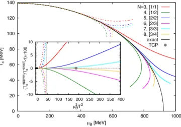
We can sample T_c at imaginary values of μˆB and fit multipoint Pad´e approximants to the sampled data (see AppendixA). Then, we can evaluate the Pad´e approximant at real values of μˆB and compare the value of analytic continuedT_c with the exact values obtained from(7). This comparison is presented in Fig.1, where the inset shows the percentage difference between C_Nðμˆ²_BÞ and T_cðˆμ²_BÞ using the same interpolating points as those shown in Fig. 3in the case of the QCD data. The main figure shows that the diagonal sequence converges from above, while the

0 20 40 60 80 100 120 140

0 200 400 600 800 1000

Tc [MeV]

PB [MeV]

N=3, [1/1]

4, [1/2]

5, [2/2]

6, [2/3]

7, [3/3]

8, [3/4]

exact TCP

-10 -5 0 5 10

0 50 100 150 200 250 300 350 400 (Tc approx/Tc exact-1)u100

PB 2/T²

FIG. 1. Apparent convergence of the multipoint Padé approx- imantsC_N (solid lines) determined fromT_c values atμÎB in the CQM model in comparison to the Taylor expansion of orderN−1 around μB¼0 (dashed lines). In the main plot the parametric curves for the Padé approximants are obtained asð ffiffiffiffiffi

ˆ μ²B

p C_Nðμˆ²BÞ;

C_Nðμˆ²BÞÞ. The bivaluedness of the subdiagonal approximants (and the curves of the odd-order Taylor expansion) reflects thatffiffiffiffiffi μB≔

ˆ μ²B

p C_Nðμˆ²BÞ has a maximum. The inset shows the percentage difference between the approximated and exact values ofT_c, with the vertical dotted line indicating the radius of converges of the Taylor expansion.

4These expressions corresponds to Eqs. (13) and (14) of[41], just that we used the relation _∂n^∂ðLi_nð−e^zÞ þLi_nð−e^−zÞj_n¼0¼

−γ−lnð2πÞ−½Ψðð1þiz=πÞ=2Þ þΨðð1−iz=πÞ=2Þ=2, which can be proven by comparing the high temperature expansion used there with the one given in[42].

(6)

subdiagonal sequence converges from below to the line m²_eff ¼0, which forμB<μ^TCBB is the line of critical points and for μB >μ^TCB_B is the first spinodal. Given that the sampling range is μˆ²B∈ð−7.35;0, the accuracy of the

½3=4Pad´e approximant around the location of the TCP is remarkable, even thoughT_cðμˆ²BÞis a rather simple function, as it represents an ellipse. This is even more so when one compares to the radius of convergence of the Taylor expansion around μB¼0 which is μˆ²_B≈44.2, as given by the pole in(7). We only refer to the TCP becauseμB(or

ˆ

μ²_B) is rather large there; the Pad´e approximant does not know about the existence of the TCP, as this is encoded in the quartic part of the tree-level potential and the second derivative ofhqqi=¯ Φ(qis the constituent quark field) with respect toΦ, which jointly determine λeff.

2. Effect of the error

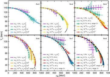
Next, we investigate what happens when analytic continuation is performed in the presence of noise. As a reference point we start by generating Tⁱ_c configurations with a normal distribution characterized by mean calculated from (7) and standard deviation corresponding to the relative errorw_Tⁱ_c=Tⁱ_c ¼1%and investigate to what extent should we decrease the relative error in order to get close to the curves obtained in Fig.1in the absence of noise. Note thatw_Tⁱ_cis by a factor of two larger than the average error of the QCD data at imaginary chemical potential.

We determine the coefficients of the multipoint Pad´e approximant for each generated configuration, evaluate the approximant for positive μˆ²B and, using the Bayesian method presented in Sec. II B, calculate χ² including or omitting information on the Taylor coefficients, and then study the posterior distribution of these values. The method is applied to the QCD data in the next subsection, where it is referred to as Method 1. The control points used to calculate χ² have μˆ²_B corresponding to the QCD data at imaginary chemical potential andT_cobtained from(7). We use a unique relative error of T_c at all interpolating and control points, whose value is indicated in the key of Fig.2 (w_Tⁱ_c used to generate Tⁱ_c instances is twice the indicated value). When Taylor coefficientsc₁andc₂are also used in the calculation of χ², their values c₁¼−1.575 andc₂¼ 0.0267is determined from the Taylor expansion of(7), as for the reference value of their error, indicated in the key of Fig. 2, we use the error of the QCD data obtained from Ref. [2], namely σ⁰c₁ ¼0.626and σ⁰c₂¼0.627. The sampling points in the range μˆ²B∈ð−7.35;0 are those used previously to obtain Fig.1. We also investigate the effect of changing the sampling range for fixed value of the error by increasing the lower bound of the interval by the factor indicated in the keys of Fig.2. In the modified range the interpolating points are equidistant from each other.

Worth noticing in Fig.2is that in the presence of noise the bands forT_cðμBÞcan deviate above some value ofμBfrom

the curves of Fig.1by more than the estimated statistical error. This reflects the ill-posedness of the analytic continuation problem. However, even with the largest error used, the Pad´e sequence converges up toμB≈600MeV.

For the mathematically curious, we also show the effect of increasing the range of the interpolation points. As expected, convergence is accelerated by the increase of the sampling range. This is of course not directly relevant for QCD, as the Roberge-Weiss transition puts a limit on the available range for the interpolation points.

B. Analytic continuation of QCD data

We apply he method presented in Sec. II to the continuation of the critical line of the QCD in the T− μBplane. Our main focus is the study of the convergence of Pad´e series of the form½p=p and½p=pþ1 constructed:

(1) based only on interpolating points (multipoint Pad´e approximants), or

(2) using interpolating points and the expansionfðtÞ≈ c₀þc₁tþc₂t² around t¼0, as explained in Sec.III A (Pad´e-type approximant).

We use the continuum extrapolated values ofT_c recently determined on the lattice atμB ¼0 and seven imaginary values ofμˆB¼μB=T, namely

ˆ

μBðjÞ ¼ijπ

8 ; j¼0;2;3;4;5;6;6.5;7; ð8Þ given in Table II of[3]and the Taylor coefficientsκ₂andκ₄, appearing in the parametrization

T_cðμBÞ ¼T_cð0Þ½1−κ₂ðμB=T_cð0ÞÞ²−κ₄ðμB=T_cð0ÞÞ⁴; ð9Þ also extrapolated to the continuum limit in[2].

40 60 80 100 120 140

160 _N=3

PB [MeV]

w_Tci: 1.0%, V_ci=V_ci⁰ w_Tci: 0.1%, V_ci=V_ci⁰ w_Tcⁱ: 0.1%, V_ci=V_ci⁰/10 w_Tci: 0.01%, V_ci=V_ci⁰/10²

N=4

w_Tci: 1.0%, V_ci=V_ci⁰ w_Tci: 0.1%, V_ci=V_ci⁰/10 w_Tcⁱ: 10^-3%, V_ci=V_ci⁰/10³ w_Tci: 10^-4%, V_ci=V_ci⁰/10²

N=5

w_Tci: 1.0%, V_ci=V_ci⁰ w_Tci: 0.1%, no ci w_Tci: 0.1%, no ci, range: 2u w_Tci: 10^-3%, V_ci=V_ci⁰/10³ w_Tci: 10^-4%, V_ci=V_ci⁰/10⁴ w_Tci: 10^-5%, V_ci=V_ci⁰/10⁵

20 40 60 80 100 120 140

0 200 400 600 800 1000 N=6

w_Tci: 1.0%, V_ci=V_ci⁰ w_Tci: 0.1%, V_ci=V_ci⁰ w_Tcⁱ: 10^-3%, V_ci=V_ci⁰/10³ w_Tci: 10^-4%, V_ci=V_ci⁰/10⁴ w_Tci: 10^-5%, V_ci=V_ci⁰/10⁵, range: 3u

200 400 600 800 1000 N=7

w_Tcⁱ: 1.0%, V_ci=V_ci⁰ w_Tci: 0.1%, no c_i w_Tci: 10^-5%, no ci w_Tci: 10^-5%, no ci, range: 2u w_Tci: 10^-7%, no c_i w_Tcⁱ: 10^-7%, no ci, range: 2u

200 400 600 800 1000 T [MeV]c N=8

w_Tcⁱ: 1.0%, V_ci=V_ci⁰ w_Tci: 0.1%, V_ci=V_ci⁰/10 w_Tci: 10^-3%, V_ci=V_ci⁰/10³ w_Tci: 10^-5%, V_ci=V_ci⁰/10⁵ w_Tci: 10^-6%, V_ci=V_ci⁰/10⁶, range: 3u w_Tcⁱ: 10^-7%, no ci, range: 2u

FIG. 2. Result of a mock analysis showing the effect of the error of the data and of the sampling range on the quality of the analytic continuation obtained via multipoint Pad´e approximants of various order and by including or omitting information (the latter is denoted by“noc_i”in the key) on the error of the Taylor coefficients in the evaluation ofχ². For additional information see the main text.

(7)

With the notation of Sec.II, the (assumed) functionfðtÞ, which corresponds to T_cðμˆ²BÞ, is known at seven points τj¼μˆ²_BðjÞ<0, corresponding toj≠0in the list given in (8), and we also know c₀¼T_cðˆμBðj¼0ÞÞ, as well as c₁ andc₂in terms ofκ2andκ4. The values ofκ2,κ4andT_cð0Þ reported in[2]give through the explicit relations given in Appendix B c₁¼−1.878 and c₂¼0.0451 with errors σc₁ ¼0.626andσc₂ ¼0.627.

1. Numerical implementation of the Bayesian approach In order to use the method presented in Sec.III A, we need to generate fTⁱ_cg instances at chosen interpolating points (also values ofc₁andc₂in the case of the Pad´e-type approximant) and then evaluateχ², defined in(4), using the actual lattice data as control points. The interpolating points

ˆ

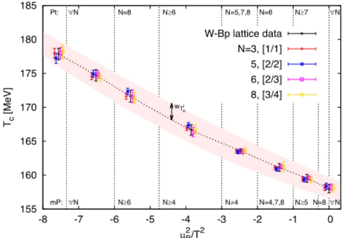
μ²B;iused for the two types of Pad´e approximants mentioned above are indicated in Fig. 3. The idea behind our choice was that each interpolating point of any of the used approximant fall in between two nearby lattice data points and be more or less equally distributed in the sampling range. The actual choice of the interpolating points is not important, however, in order to maximize the sampling range, one interpolating point is chosen close to the lattice data point with μˆ²_Bðj¼7Þ and, since we are interested in

analytic continuation through μB¼0, we also choose ˆ

μ²Bðj¼0Þ ¼0as an interpolating point.

We use two methods to generate input for the Padé approximants. In the first method (Method 1) we simply generateTⁱ_c from normal distribution with mean obtained by interpolating the mean of the lattice data and with the standard deviation (SD) indicated in Fig.3. In this casec₁ andc₂, used in the Padé-type approximant, are generated from a normal distribution with mean and SD given by Eqs.(B2)and(B3), respectively. As a result,c₁andc₂are taken into account in the calculation ofχ²only when using the multipoint Padé approximant. According to our prior, we only accept those configurations for which the corresponding Padé approximant is free of spurious poles in the wide rangeμˆ²B∈½−π²;60π². When using this method we calculateT_cat some value ofμˆ²_BasT_c¼Rⁿ_mðμˆ²_BÞand the value of the real chemical potential as μB ¼ ffiffiffiffiffi

ˆ μ²B

p T_c and determine their percentile based error using the weighte^−χ²⁼². The second method (Method 2) for generating input for the Padé approximants is the importance sampling using the Metropolis algorithm with“action”χ²=2. The proposed value of Tⁱ_c in the Markov chain is generated using a normal distribution for the noise with vanishing mean and SD of Oð1ÞMeV. In the case of the Padé-type approximant we use normal distribution with standard deviationσci; i¼1, 2 to generate the noise for the Taylor coefficients c_i. Configurations for which the corresponding Padé approximant has spurious poles in the range given above are excluded by assigning to them the value χ²¼∞. For the remaining configurationsχ² is calculated using all the available lattice data according to the formulas in(4). The average and percentile based error ofT_c ¼Rⁿ_mðˆμ²BÞandμBfor the Padé approximants were calculated in the standard way with the configurations provided by the Metropolis algorithm.

There are some peculiarities when doing importance sampling in this context. These are related to the spurious poles of the Pad´e approximants, which appear as“walls”of infinite action in the Metropolis update. Configurations with spurious poles are not guaranteed to be isolated points in the space of all configurations, rather, there can be regions in configurations space where all approximants have a pole.

One can easily stumble on an accepted configuration that is surrounded in most directions by configurations with a pole, thereby trapping the algorithm. To avoid this problem it is a good idea to mark out a temperature range sampled by the algorithm during the random walk and assign infinite value for the action if a proposedTⁱ_clies outside this range. I.e., even in the case ofMethod 2a prior, like that in Fig.3is used. An other reason to introduce this band is to exclude the Pad´e approximants from having features in the interpolated range not present in the data, even if such an approximant has no pole and fits the data points acceptably. This is also a possibility, since Pad´e approximants are rather flexible. In practice a two times wider band than the one shown in Fig.3proved sufficient.

155 160 165 170 175 180 185

-8 -7 -6 -5 -4 -3 -2 -1 0

Tc [MeV]

PB 2/T²

W-Bp lattice data N=3, [1/1]

5, [2/2]

6, [2/3]

8, [3/4]

mP:

Pt:

wT_cⁱ

N Nt6 Nt4 Nz4 N=4,7,8 Nt5 N=8 N

N N=8 Nt6 N=5,7,8 N=6 Nt7 N

FIG. 3. Choice of the interpolating (node) points, whose position is indicated by the vertical dotted line, in comparison to the actual lattice data. The labels indicate the use of the interpolating point in the multipoint Padé approximant (bottom) and the Padé-type approximant (top) of a given order, characterized by the number of independent parametersN. At the value ofμˆ²Bcorresponding to the lattice data points we show the mean and the error of the T_c computed from the multipoint Padé approximants generated with importance sampling (for the sake of the presentation the abscissa is shifted). The band indicates the standard deviation of the normal distribution used inMethod 1to generatefTⁱ_cg instances, i.e., it indicates the prior distribution, excluding the factor that removes the spurious poles. The values

¯

T_cðμˆ²B;iÞat the node pointsμˆ²B;iused in the expression(5)of the prior are from the dotted curve in the band, which interpolates the mean values of the lattice data.

(8)

Another observation is that in some cases it was very hard to thermalize the system by updating the value ofT_c only at one interpolating point at a time. It proved more useful to propose in the Metropolis algorithm an updated array of T_c values, as this procedure also substantially reduced the autocorrelation time.

2. Results for the analytic continuation

The first thing worth checking is the distribution ofT_c calculated from the Padé approximants atμˆ²B values corresponding to the actual lattice data points. For the majority of the approximants and lattice data points, the distribution is very close to a normal one with standard deviation com- patible with that of the lattice data. The latter can be seen in Fig. 3 in the case of the multipoint Padé approximant, meaning that the selection of theT_cinstances based onχ² works as expected. However, different low order approximants seem to select, within the error, different ranges in the distribution ofT_c(andc_iwhen the Padé-type approximant is used). This is most visible in the case of the [2/2] approximant where the points posses a structure unseen in the lattice data. The multipoint Padé approximant [1/1] is the most constrained by the likelihood, the error of T_c being smaller than the lattice one, while the [3/4] approximant is the least constrained, matching closely the lattice error at all lattice points, and showing a wider range of the computedc₁ andc₂coefficients. This loss of constraint is also reflected by theχ²histogram whose pick moves to higher values when the number of parameters of the approximant increases.

Now we turn our attention to the extrapolation. Since both Method 1andMethod 2used to generate input for both the multipoint Padé and Padé-type approximants resulted in very similar results for the analytically continuedT_cðμBÞcurve, we only present those obtained with Method 2 (importance sampling) in the case of the Padé-type approximant constructed using the first and second derivative ofT_cðμBÞ at μB ¼0. The fact that withMethod 1the analytic continuation does not depend on the approximant used, means that it makes no difference whether we take into account the Taylor coefficients only in the approximant or only in the calculation ofχ². We remind that when importance sampling is used the Taylor coefficients are taken into account in the calculation of χ²irrespective of the type of approximant, since otherwise the range in which c₁ and c₂ varies during the random walk would not be constrained.

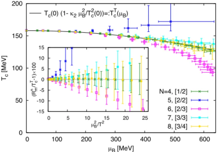
Our main result on the analytic continuation is presented in Fig.4in comparison with a simple parametrization of the crossover line based on the Taylor coefficientκ₂. One sees that with the exception of the [2/2] type, the Pad´e approximants tend to give smallerT_c with increasingμB. Also, the behavior of the diagonal an subdiagonal sequences follow different patterns, similar to that observed in the model study in Fig. 1. Apparently, the Pad´e sequences converge, as, although [3/3] and [3/4] have overlapping error bars of similar size, the latter moves toward the band

laid out by the [2/3] approximant. It remains to be seen if this pattern survives the possible addition of new lattice data points, which will further constrain the fit, and/or an increase in the precision of the lattice data.

IV. CONCLUSIONS AND OUTLOOK We presented a method for the numerical analytic continuation of data available at imaginary chemical potential that uses also the Taylor coefficients of an expansion around μB¼0. Using lattice data that became available recently, we have investigated the continuation to realμBof the crossover line with a sequence of Pad´e approximants, looking for apparent convergence as the number of independent coefficients increases. Such an analysis would have been less conclusive using the smaller data set available at imaginaryμB in[31] and without taking into account the lattice data for the Taylor coefficients.

Our largest order Pad´e approximants is very close to the simplest quadratic curve obtained with just theκ₂coefficient.

This means that if the observed apparent convergence is genuine, such a quadratic approximation might be applicable in a rather large range ofμB. We would like to stress that, as discussed in the case of an effective model in Sec.III A, our results on the analytic continuation tell nothing on the possible existence and location of the critical end point (CEP). It is also not possible to clearly determine the value ofμBup to which the analytic continuation could be trusted.

The Taylor and imaginary chemical potential methods are usually considered to be competitors in the study of finite density QCD. This is somewhat unfortunate, as the two methods tend to provide complimentary information.

With the Taylor method, lower order coefficients tend to be more precise, while data at imaginaryμB tends to restrict higher order coefficients better, without giving a very

0 50 100 150 200

0 100 200 300 400 500 600

T_c(0) (1- N2P²B/T_c²(0))=:T_c^T(PB)

Tc [MeV]

PB [MeV]

N=4, [1/2]

5, [2/2]

6, [2/3]

7, [3/3]

8, [3/4]

-15 -10 -5 0 5 10 15

0 5 10 15 20 25

(Rmn /TcT-1)u100

PB 2/T²

FIG. 4. Result of the analytic continuation via the diagonal and subdiagonal sequences of Pad´e-type approximants constructed based onfTⁱ_cginstances generated using importance sampling.

The inset shows the percentage difference with respect to the T_cð0Þð1−κ2μ²B=T²_cð0ÞÞ curve plotted in the main figure, for which we usedT_cð0Þ ¼158.01MeV andκ2¼0.012.

(9)

precise value for the lower orders. For the case of baryon number fluctuations, this can clearly be seen by comparing Fig. 3 of Ref.[27], where the signal forχ^B₆ andχ^B₈ is better, with Fig. 1 of Ref. [43], whereχ^B₄ is much more precise.

This means that joint analysis of such data might be a good idea also for the equation of state, where there are some indications—both from an explicit calculation on coarser lattices[44–46]and phenomenological arguments[47–49]

—that the radius of convergence for temperatures close to the crossover is of the order μB=T≈2, making a Taylor ansatz unusable beyond that point. This makes it mandatory to try different ansatze, or resummations of the Taylor expansion, and one possible choice could be the Pad´e approximation method used here.

ACKNOWLEDGMENTS

We would like to thank Sz. Borsányi, M. Giordano, S. Katz and Z. Rácz for illuminating discussions on the subject and J. Günther for providing the raw lattice data of [31]in an early stage of the project. This work was partially supported by the Hungarian National Research, Development and Innovation Office—NKFIH Grants No. KKP126769 and No. PD_16 121064, as well as by the DFG (Emmy Noether Program EN 1064/2-1). A. P. is supported by the János Bolyai Research Scholarship of the Hungarian Academy of Sciences and by the ÚNKP-20-5 New National Excellence Program of the Ministry of Innovation and Technology. In an early stage this research was also supported by the Munich Institute for Astro- and Particle Physics (MIAPP) of the DFG cluster of excellence

“Origin and Structure of the Universe”.

APPENDIX A: THE MULTIPOINT PADÉ APPROXIMATION METHOD

Following Refs. [38,50], we briefly summarize the construction of the multipoint Pad´e approximant used to analytically continue functions known only at a finite number of points of the complex plane. In our case the continuation is done along the real axis, from negative to positive values.

When one knows the function at N points f_i¼fðz_iÞ;

i¼0…N−1, the rational function approximating fðzÞ is most conveniently given as a truncated continued fraction

C_NðzÞ ¼ A₀ 1þ

A₁ðz−z₀Þ

1þ A_N−1ðz−z_N−2Þ

1 ; ðA1Þ

where we used the notation _1þ¹ x≡_1þx¹ . The task is to determine the N coefficients A_i from the conditions C_Nðz_iÞ ¼f_i, i¼0…N−1. Note that only N−1 values of z_i appear in (A1), z_N−1 appears in the condition C_Nðz_N−1Þ ¼f_N−1. The coefficients can be obtained effi- ciently as A_i¼g_iðz_iÞ, i¼0…N−1, with the functions g_iðzÞdefined by the recursion

g_pðzÞ ¼g_p−1ðz_p−1Þ−g_p−1ðzÞ

ðz−z_p−1Þg_p−1ðzÞ ; 1≤p≤N−1; ðA2Þ with initial conditiong₀ðzÞ ¼fðzÞ, which meansg₀ðz_iÞ ¼ f_i, when the function is known only in some discrete points. Working out explicitly the conditionA_i¼g_iðziÞfor a few values ofi, one sees that one needs to construct an upper triangular matrix t_i;j using the recursion t_i;j¼ ðt_i−1;i−1=t_i−1;j−1Þ=ðzj−z_i−1Þ, for j¼1;…; N−1 and i¼1;…; j, starting from its first row t_0;j¼f_j, j¼0;…; N−1. The diagonal elements are the coefficients ofC_N: A_i¼t_i;i. The relation of C_N with the Pad´e sequence is as follows: ifN≥1is odd, thenC_N ¼ ½p=p withp¼ ðN−1Þ=2, while whenN ≥1is even, thenC_N ¼

½p=pþ1 withp¼−1þN=2.

Writing C_NðzÞ in the form C_NðzÞ ¼NðzÞ=DðzÞ, the numerator and denominator (at a given value ofz) can be easily determined from the coefficients of the truncated continued fraction via the following three-term recurrence relation

X_nþ1¼X_nþ ðz−z_nÞA_nþ1X_n−1; ðA3Þ where for the numerator (X¼N) one hasX₁¼0,X₀¼A₀ and for the denominator (X¼D) one has X₁¼X₀¼1, and the iteration goes from n¼0 up to and including n¼N−2. The coefficients a_i (b_i) of the numerator (denominator) can be easily obtained by calling the above recursion(A3)at a finite number of pointszand solving a system of linear equations.

APPENDIX B: RELATING c_1;2 WITH κ2;4

In order to relate the coefficientsc₁andc₂of the Taylor expansion T_cðtÞ ¼c₀þc₁tþc₂t², with t¼μˆ²_B, with the coefficientsκ₂andκ₄used by the HotQCD Collaboration, the expansion(9)has to be rewritten in terms ofμˆ²B∶

T_cðμBÞ

T_cð0Þ ¼1−κ2T²_cðμBÞ

T²_cð0Þ μˆ²B−κ4T⁴_cðμBÞ

T⁴_cð0Þ μˆ⁴B: ðB1Þ Then, using that T²_cðμBÞ=T²cð0Þ≈1–2κ2μˆ²B and T⁴_cðμBÞ=

T⁴_cð0Þ ¼1þOðμˆ²_BÞ, we obtain

c₁¼−κ₂T_cð0Þ and c₂¼ ðκ₄−2κ²₂ÞT_cð0Þ: ðB2Þ Ignoring the covariance between κ₂ andκ₄, which is not known to us, the error associated to these Taylor coefficients are

σc₁ ¼ ½T²_cð0Þσ²_κ₂þκ²₂σ²_T_c_ð0Þ¹²;

σc₂ ¼ ½T²cð0Þðσ²κ4þ16κ²₂σ²κ2Þ þ ðκ²₄þ4κ⁴₂Þσ²_T_c_ð0Þ¹²: ðB3Þ Inc₁andc₂and their errors we use the data of the HotQCD Collaboration also forT_cð0Þ.