hjic.mk.uni-pannon.hu DOI: 10.33927/hjic-2020-03
THEORETICAL BACKGROUND AND APPLICATION OF MULTIPLE GOAL PURSUIT TRAJECTORY FOLLOWER
ERN ˝OHORVÁTH*1,2, CLAUDIUPOZNA3, PÉTERKORÖS˝ 2, CSABAHAJDU2,ANDÁRONBALLAGI2
1Department of Computer Engineering, Széchenyi István University, Egyetem tér 1, H-9026 Gy ˝or, HUNGARY
2Research Center of Vehicle Industry, Széchenyi István University, Egyetem tér 1, H-9026 Gy ˝or, HUNGARY
3Faculty of Electrical Engineering and Computer Science, Transilvania University of Brasov, B-dul Eroilor nr.
29, 500036 Brasov, ROMANIA
Autonomous and self-driving technology is a rapidly emerging field among automotive-related companies and academic research institutes. The main challenges include sensory perception, prediction, trajectory planning and trajectory execu- tion. The current paper introduces a design strategy and the mathematical background of the optimization problem with regard to the multiple goal pure pursuit algorithm. The aim of the algorithm is to provide a low degree of computational complexity and, therefore, a fast trajectory-tracking approach. Finally, in terms of our approach, not only the theoretical questions but the application challenges will be described as well.
Keywords: autonomous, self-driving, algorithm, trajectory-tracking
1. Introduction
The current paper deals with the design strategies, the- oretical background and application of trajectory track- ing. The trajectory-follower approach that is discussed is called the multiple goal pure pursuit algorithm, in partic- ular the windowed version. In mobile robots or vehicles, the trajectory design strategy seeks to identify the best possible trajectory which approximates a desired trajec- tory based on waypoints. This also assumes that the tra- jectory design phase has already created the desired tra- jectory.
This paper is organized as follows. The first section introduces the general problem and summarizes the state- of-the art and most relevant results. The second section deals with the design strategy of trajectory tracking and defines the problem precisely. The third section defines the optimization problem and possible solutions, while the fourth section summarizes the results. Finally, the last section includes a summary and conclusions.
The current state-of-the-art results The essence of pure pursuit is to choose a look-ahead point from the de- sired trajectory in front of the vehicle and steer accord- ing to it. This simple idea can be realized in many differ- ent ways, e.g., the classical pure pursuit algorithm uses a fixed look-ahead distance. This means that on the given track, a look-ahead point can be determined as a subset
*Correspondence:herno@ga.sze.hu
of waypoints, which are a fixed distance from the vehi- cle. Choosing a look-ahead distance is a tradeoff between control overshoots and precision. If the look-ahead dis- tance is small, the overshoot will appear because the cho- sen point is so close that the vehicle cannot react instanta- neously, thus continuously exceeds its target. In this case, the absolute distance (error) is smaller but the vehicle will oscillate. In contrast, if the chosen point is too far away, the vehicle will follow the point after the following corner so cuts off the bend. This behavior can be eliminated if the look-ahead distance is adjustable or changeable. One of the most obvious ways to modify the look-ahead dis- tance is to scale the speed of the vehicle accordingly [1].
The other method of modifying the look-ahead distance involves a fuzzy controller that automatically adjusts the look-ahead distance based on path characteristics, veloc- ity and tracking errors [2,3]. Similarly to the fuzzy ap- proach [4], it was shown that an autonomous vehicle can drive at a velocity of approximately80 km/h along ex- plicit paths using differential GPS data. To improve the classical pure pursuit algorithm and eliminate steering latency, CF-Pursuit [3] replaced the circles employed in pure pursuit with a clothoid curve to reduce fitting errors.
Although many papers have examined this domain, the available source code is rather rare. A few of the most notable versions are Autoware [5], Python [6] and Rap- tor Unmanned Ground Vehicle (UGV) [7]. Our research group also introduced a pure pursuit method based on multiple look-ahead points [8], in this paper its updated
version will be presented.
2. The design strategy
The motivation of our research was to construct a simple but flexible kinematic trajectory tracking approach. In ad- dition, the implementation of amore human-like thinking was sought, in other words, to track and follow more goal points on a road simultaneously. Drivers also take mul- tiple considerations into account, e.g., not only is lane- keeping an important task but a cyclist in the same lane also influences planning. In our previous work the multi- ple goal pursuit algorithm can be viewed as a supplement to the pure pursuit algorithm. The most significant change was the calculation of curvature. Assuming the reference trajectory is given with a set of geometric pointsT, posi- tionP, steering angleγand orientationθof the vehicle, G⊆T is defined as the set of selected goal points with a preset lengthN =|G|:
G={G1, G2, . . . , GN|Gk,(l+o)≤k <(l+o+N)}
(1) An angle αf from a domain of possible angles [αmin, αmax] is assumed (presumably the wheel angle limits). A sequence of curvatures can be calculated each with a radius pf = −2/αand a centre pointCf. A goal pointGkfrom setGto anyCfdetermines a line segment:
the normalized difference between the length of this seg- ment and radiuspfis the distanced ∈R+from the cur- vature. The metric for selecting a good angle is the sum of this difference for each goal point.
dsum=
N
X
k=0
−−−→CfGk
−ρf
. (2) Heredsumdenotes the total distance for goal point setG.
The aim is to minimize this distance.
This paper introduces a new approach to the multiple goal pure pursuit algorithm, which is based onwindow- ing. This algorithm is not regarded as a classical trajec- tory tracker since it slightly redesigns the original trajec- tory. With this method, a trajectory similar to the origi- nal one is created, but slight modifications render it more suitable for our vehicle to track. The design strategy con- sists of identifying the optimum trajectory which approx- imates a desired trajectory defined by a set of chosen points. This means that the aforementioned set is initial data and a minimum problem must be defined.
From the multitude of possibilities, the minimum problem will be defined starting with the following hy- pothesis:
1. During the approximation, the steering angle γ is constant;
2. Changing the steering angle γ is an instantaneous process.
If the previous hypotheses are correlated, it can be con- cluded that the initial set of points is approximated by a
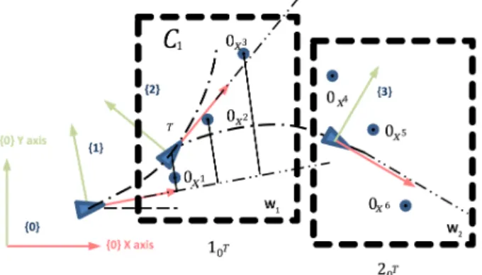
Figure 1:The windowed goal pursuit strategy
trajectory composed from arcs of a circle. The transition from one arc to another is instantaneous. For a particular arc of the circle, a subset (referred to here as theworking set) is selected from the initial set.
The following decisions are subjects of debate:
• The number of points included in the working set;
• The number of commune points which belong to dif- ferent working sets;
• The position of the car when the next working set is defined.
The aforementioned observations are shown in Fig. 1, where a possible strategy is illustrated. The figure con- tains two referential systems. The first, 0, is the global (stationary) referential system; the second,1,2,3, is the mobile referential system attached to the vehicle. The blue triangles denote the abstraction of the vehicle. Two windows are labelled as w1,2. Each of them contains a working setof three points.
The trajectory is a composition of two arcs of a circle, C1andC2. The first (C1) is defined in referential frame 1using the windoww1, i.e., the points0x1,0x2and 0x3. The second (C2) is defined in referential frame2 using the windoww2, i.e. the points0x4,0x5 and 0x6. Each of the mentioned points is defined in referential frame0.
3. The optimization problem
Using m windows and n points for each window, the mathematical definition of the problem is
Rj = arg min
m
X
i=1
ei
!
, (3)
whereRjdenotes the radius of arcCj,eistands for the distance from pointito arcCj,j represents the current window numberj = 1, . . . , m, andiis the current point number which belongs to windowj.
The distance from point xi toCj is also debatable.
Fig. 2illustrates two possibilities: the first (Fig. 2a) only considers one coordinate of the current point. In contrast, inFig. 2bthe shortest distance is considered.
Figure 2: Possible ways of computing the distances
For the first choice:
ei=yi−Cj(xi), (4) where
jxi
jyi 1
=j0T0xi=
cθ −sθ 0 sθ cθ 0
0 0 1
xi yi 1
0xi; (5) θdenotes the orientation of the referential systemj; and xj, yj represent the coordinates of the origin of referen- tial systemj.
If this definition is assumed, it is evident that this is a quadratic regression problem with the analytical solution
1
R =κ= XtX−1 XtY
, (6)
where
X=
x21+y21 . . . x2n+yn2
(7)
Y=
2y1
. . . 2yn
(8) For the second choice:
ei=
R−
xi
yi−R
=
R− q
x2i + (yi−R)2 (9) which has a numerical solution.
3.1 Algorithm flowchart
InFig. 3, a flowchart is presented in order to understand the approach more comprehensively.
The algorithm uses the vehicle parameters, pose, tra- jectory points and input parameters as inputs. The vehicle parameters are wheelbaseb, steering angleγand its po- sition. Also, the points:0xk are part of the initial data.
The algorithm parameters are: working setn, skylined and curvature limit. This limit decides whether the loco- motion is based on a linear or circular trajectory window.
For every iteration, a new window is calculated.
4. Discussion 4.1 Simulation
The simulation uses the previous algorithm for a kine- matic model which is in accordance with the starting hy-
Figure 3: Algorithm flowchart
xu X(k)
X(k+ 1)
xu+1 X(k+ 2)
xu+2 xu+3 e(k)
Figure 4: The definition of lateral deviation
pothesis, i.e., the steering is instantaneous. In the first simulation, the following kinematic bicycle model
˙
x=vcos (θ)
˙
y=vsin (θ) θ˙= v
Ltan (γ) γ=ct
(10)
was used. To analyze the results, the lateral approxima- tion error was defined:
• The lateral deviation error of the current position e(k)is the distance between this position and the current segment of the desired trajectory (Fig. 4);
• The total deviation erroreT is the sum of the error throughout the simulation from1toN;
• The relative deviation erroreris the ratio of the total error to the total number of simulated points.
e(k) = distance
x(k),0xu0xu+1
=
=
x(k)xu+1−x\uxu+1
x(k)xu+1·xuxu+1 (11) eT =
N
X
k=1
e(k) (12)
er=eT
N (13)
These errors are dependent on the number of points in- cluded in the working set (n) referred to as the skyline and the position of the decision point (d). For the desired trajectory, a study relative to this dependency was con- ducted and the relative errors for each case were obtained (n, d).
The non-instantaneous steering was also simulated (Fig. 5). In this case, the kinematic bicycle model can be modified as follows:
˙
x=vcos(θ)
˙
y=vsin(θ) θ˙= v
Ltan(γ) γ=γ0+ ˙γt
˙ γ=ct
(14)
The steering angle is a linear function where the steer- ing velocity is constant during the steering process. The
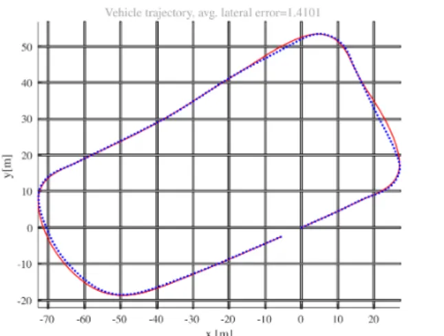
Figure 5: Simulation result: the blue dots denote the way- points, the red line represents the trajectory generated by our model
trajectory of the robot is no longer an arc of a circle but a combination of two curves. The first of which is a clothoid (also referred to as an Euler spiral) when γ = γ0+ ˙γt and an arc of a circle when γ = ct. In this case, the simulation result shows a lower quality of approximation. Given this phenomenon, the robot orien- tation angle error is defined as the difference between the orientation angle in the hypothesis where the steering is instantaneously modified to the final value and the orien- tation angle in the hypothesis where the steering angle is continuously modified from the initial to the final value.
eθ= v
L tan (γf) ∆t− Z ∆t
0
tan(γ0+ ˙γτ)dτ
!
=
= v
˙ γL
tan (γf) ∆γ−log
cos(γ0) cos(γf)
(15) where γ0 denotes the initial steering angle, γf = arctan(Lκrepresents the final steering angle, γ˙ stands for the steering angle velocity, and∆tis the steering time.
It is observed that Eq. 12is in accordance with our intuitions: if the steering angle velocity increases the ori- entation error angle will decrease; in contrast, the velocity is proportional to the error.
A strategy where a maximum orientation erroreθmax is allowed can now be contemplated and since the maxi- mum steering velocityγ˙ is an actuator parameter (which is constant), the following function for the vehicle veloc- ity is proposed:
vnew =eθmax eθ
vold. (16)
In conclusion, the algorithm must be improved in order to yield better results. The following possibilities are sug- gested (Fig. 6):
• Refine the input set of points: interpolate new points;
• Change the vehicle velocity during locomotion (Eq.
16);
Figure 6: The proposed new strategy
• Define the new windows by including the points which succeed the decision point in the new working set.
With regard to an examined sample trajectory, a 3D graph (Fig. 7) is provided which shows the relative dependency obtained in terms of the relative error value in each case (n, d). InFig. 7, thexaxis denotes the skyline (n), the
Figure 7: The relative error depends on the skyline (n) and decision point (d)
Figure 8: Typical behaviors of the examined approaches
y axis represents the decision point (d), and thez axis stands for the relative error.
4.2 Experiments
Firstly, the behavior of the algorithm in its own simu- lation environments was tested; the two presented ap- proaches (the plain multiple goal pursuit and the win- dowed multiple goal version) were developed in paral- lel in Python and MATLAB. These simulations also used real-world trajectories and the vehicle model was first a kinematic, and later a dynamic one. Subsequently, it became necessary to even test the algorithms in Open Source Robotics Foundation’s (OSRF) Gazebo for two reasons. Firstly, implementation of the algorithm as a Robot Operating System (ROS) node was sought and sec- ondly, a more precise dynamic model of the vehicle al- ready existed in Gazebo. Gazebo also facilitated the inte- gration of the useful software as well as agile migration between development and target.
For these purposes, the algorithm had to be recreated in C++ not only because of the ROS compatibility but computational resources as well. Simulation-based exe- cution yielded no significant deviation from the simulated tests. In Fig. 8, some of our results are shown regard- ing the examined trajectories. Thex andy axes are in meters. This simulation is based on real-world measure- ments taken at the ZalaZone Automotive Test Track in Zalaegerszeg and the GPS coordinates are assigned us- ing Universal Transverse Mercator (UTM) because of the minimal degree of distortion involved. The Follow the Carrot and speed ratio-based pure pursuit algorithms had to be implemented in order to experiment with them in the same environment.
In another experiment, autonomous functionalities were installed in an electric vehicle (Nissan Leaf).Fig.
9represents the vehicle in operation. The operational do- main of this vehicle was limited to the ZalaZone Auto-
Figure 9: The vehicle used in our experiments
motive Test Track and the university campus, moreover, it was required to reach a relatively slow speed of25km/h.
The vehicle has front-wheel drive, with a wheelbase of 2.70meters and a track width of1.77meters. To ensure instantaneous localization of the vehicle, two highly ac- curate Real Time Kinematic (RTK)-capable GPSs were used. One was KVH’s Fiber Optic Gyro 3D Inertial Nav- igation System (GEO-FOG 3D INS), the other was Swift Navigation’s Duro Inertial RTK. These sensors were also used to capture reference trajectories.
Our software was based on OSRF’s ROS [9]. Our computing platform first features the NVIDIA Jetson TX2, later the NVIDIA Jetson AGX Xavier. Low-level control is realized by using a National Instruments’ Com- pactRIO Controller, namely cRIO-9039, as the Real-time and FPGA modules - the NI-9853 CAN, NI-9403 DI, NI- 9205 Voltage Input and NI-9264 Voltage Output Modules to be exact.
After the algorithm exhibited satisfactory behavior in the simulation environment, it was tested in a real- world scenario. During the experiment, the NVIDIA Jet- son TX2 was used in the Nissan Leaf. The NVIDIA Jet- son TX2 is a7.5-watt embedded controller in which the Ubuntu 18.04 LTS Bionic Beaver along with the ROS Melodic Morenia were used. The embedded controller had a memory capacity of8GB and memory bandwidth of 59.7 GB/s as well as NVIDIA’s Denver2, quad-core ARM Cortex-A57 CPU and integrated256-core Pascal GPU installed. During our experiments, only the KVH’s GEO-FOG 3D INS sensor was used as the source of lo- calization, the wheel angle reference signal in addition to the speed reference via CAN were provided, and the wheel angle and speed were measured back in the same protocol. Nevertheless, during acquisition of the data, all the sensory information was logged by two of Velodyne’s 16-channel LIDARs, Sick’s 1-channel Laser Measure- ment Sensor LMS111 and the camera stream into ROS bag files. The following chart (Fig. 10) shows an example of how the algorithm generated reference trajectories for two bends on the routine track, moreover, the measured wheel angle is shown.
The waypoints for the algorithm were provided by driving through a predetermined path then saving as well as filtering the position and speed data via the way- point_saver node.
In this experiment, only the multiple goal pursuit al-
-4 -2 0 2 4 6 8 10 12 14
0.00 2.00 4.00 6.00 8.00 10.00 12.00 14.00 16.00 18.00 20.00
angle (deg)
time (s) Wheel angle measurements
Wheel angle reference Wheel angle
Figure 10: Changes in the wheel angle around two bends
gorithm with one parameter set was used. This set is better compared to Autoware’s pure pursuit algorithm in terms of lateral deviation, but the speed ratio-based ver- sion worked even better. As a result, the multiple goal pursuit algorithm was able to control the vehicle with the aforementioned embedded controller at slow speeds of approximately25km/h. The algorithm is able to per- form smooth and continuous movements along a pre- defined trajectory, even maneuvering around bends and along edges.
5. Conclusion
The current paper described the development of a trajectory-tracking approach, namely the multiple goal pursuit, and summarized the mathematical and theoret- ical background needed to understand its working prin- ciples. Enhancements to and variations in the basic ap- proach are also described with regard to their benefits and weaknesses. Furthermore, a brief insight into the devel- opment process is given. Firstly, an initial version was developed in our own simulation environment, later the code became an ROS node and the simulation environ- ment was replaced by Gazebo. Finally, real-world tests showed the viability of the new algorithm, which was tested by an autonomously guided vehicle in a closed but real-world traffic environment.
One of the benefits of this algorithm is that it can be tuned more precisely around bends, moreover, it in- volves more human-like thinking, that is, tracks and fol- lows more waypoints on the road simultaneously. Fur- thermore, this approach provides quick and reliable refer- ence signals for car-like robot kinematics, thus can follow the trajectory with relatively small errors.
The discussed algorithm was implemented in MATLAB and C++ as a Robot Operating System node and our measurements were based on debug data generated by this node. This implementation is currently publicly available on GitHub in ad- dition to other measurements, videos, results and source codes: https://github.com/szenergy/
szenergy-public-resources.
Acknowledgements
The research was carried out as part of the “Autonomous Vehicle Systems Research related to the Autonomous Vehicle Proving Ground of Zalaegerszeg (EFOP-3.6.2- 16-2017-00002)" project in the framework of the New Széchenyi Plan. The completion of this project is funded by the European Union and co-financed by the European Social Fund.
REFERENCES
[1] Paden, B.; ˇCáp, M.; Yong, S. Z.; Yershov, D.;
Frazzoli, E.: A survey of motion planning and control techniques for self-driving urban vehicles, IEEE Trans. Intell. Veh., 2016, 1(1), 33–35 DOI:
10.1109/TIV.2016.2578706
[2] Ollero, A.; García-Cerezo, A.; Martinez, J.: Fuzzy supervisory path tracking of mobile reports,Control Eng. Practice, 1994,2(2), 313–319DOI: 10.1016/0967- 0661(94)90213-5
[3] Samuel, M.; Hussein, M.; Mohamad, M. B.: A re- view of some pure-pursuit based path tracking tech- niques for control of autonomous vehicle, Int. J.
Computer Applications 2016, 135(1) 35–38 DOI:
10.5120/ijca2016908314
[4] Rodríguez-Castaño, A.; Heredia, G.; Ollero, A.:
Analysis of a GPS-based fuzzy supervised path tracking system for large unmanned vehicles,IFAC
Proceedings Volumes, 2000, 33(25) 125–130 DOI:
10.1016/S1474-6670(17)39327-8
[5] Kato, S.; Tokunaga, S.; Maruyama, Y.; Maeda, S.; Hirabayashi, M.; Kitsukawa, Y.; Monrroy, A.;
Ando, T.; Fujii, Y.; Azumi, T.: Autoware on board:
Enabling autonomous vehicles with embedded sys- tems, in Proceedings of the 9th ACM/IEEE Inter- national Conference on Cyber-Physical Systems, 2018, 287–296DOI: 10.1109/ICCPS.2018.00035
[6] Sakai, A.; Ingram, D.; Dinius, J.; Chawla, K.;
Raffin, A.; Paques, A.: PythonRobotics: a Python code collection of robotics algorithms, 2018,arXiv:
1808.10703
[7] Giesbrecht, J.; Mackay, D.; Collier, J.; Verret, S.:
Path tracking for unmanned ground vehicle naviga- tion: Implementation and adaptation of the pure pur- suit algorithm, Defence Research and Development Canada (DRDC), Suffield, Alberta, Canada, 2005.
https://apps.dtic.mil/sti/pdfs/ADA599492.pdf
[8] Horváth, E.; Hajdu, Cs.; K˝orös, P.: Novel pure- pursuit trajectory following approaches and their practical, in 10th IEEE International Conference on Infocommunications (CogInfoCom), Naples, Italy, 2019.
[9] Quigley, M.; Conley, K.; Gerkey, B.; Faust, J.;
Foote, T.; Leibs, J.; Wheeler, R.; Ng, A. Y.: ROS: an open-source Robot Operating System, ICRA Work- shop on Open Source Software, 20093(2)