Financial time series
Gerencsér, László
Vágó, Zsuzsanna
Gerencsér, Balázs
Financial time series
írta Gerencsér, László, Vágó, Zsuzsanna, és Gerencsér, Balázs Publication date 2013
Szerzői jog © 2013 Gerencsér László, Vágó Zsuzsanna, Gerencsér Balázs
Tartalom
Financial time series ... 1
1. Preface ... 1
2. 1 Basic concepts ... 3
2.1. 1.1 Wide sense stationary processes ... 3
2.2. 1.2 Orthogonal processes and their transformations ... 7
2.3. 1.3 Prediction ... 11
3. 2 Prediction, innovation and the Wold decomposition ... 13
3.1. 2.1 Prediction using the infinite past ... 14
3.2. 2.2 Singular processes ... 15
3.3. 2.3 Wold decomposition ... 17
4. 3 Spectral theory, I. ... 20
4.1. 3.1 The need for a spectral theory ... 20
4.2. 3.2 Fourier methods for w.s.st. processes ... 22
4.3. 3.3 Herglotzs theorem ... 24
4.4. 3.4 Effect of linear filters ... 25
5. 4 Spectral theory, II. ... 27
5.1. 4.1 First construction of the spectral representation measure ... 27
5.2. 4.2 Random orthogonal measures. Integration ... 29
5.3. 4.3 Representation of a wide sense stationary process ... 30
5.4. 4.4 Change of measure ... 32
5.5. 4.5 Linear filters ... 33
6. 5 AR, MA and ARMA processes ... 34
6.1. 5.1 Autoregressive processes ... 34
6.2. 5.2 A classic result: the Yule-Walker equations ... 37
6.3. 5.3 The AR process ... 38
6.4. 5.4 Stable AR systems ... 40
6.5. 5.5 MA processes ... 41
6.6. 5.6 ARMA processes ... 43
6.7. 5.7 Prediction ... 45
6.8. 5.8 ARMA processes with unstable zeros ... 48
7. 6 Multivariate time series ... 51
7.1. 6.1 Vector valued wide sense stationary processes ... 51
7.2. 6.2 Prediction and the innovation process ... 53
7.3. 6.3 Spectral theory ... 54
7.4. 6.4 Filtering ... 58
7.5. 6.5 Multivariate random orthogonal measures ... 59
7.6. 6.6 The spectral representation theorem ... 62
7.7. 6.7 Linear filters ... 62
7.8. 6.8 Proof of the spectral representation theorem ... 63
8. 7 State-space representation ... 65
8.1. 7.1 From multivariate AR( ) to state-space equations ... 65
8.2. 7.2 Auto-covariances and the Lyapunov-equation ... 67
8.3. 7.3 State space representation of ARMA processes ... 70
9. 8 Kalman filtering ... 71
9.1. 8.1 The filtering problem ... 71
9.2. 8.2 The Kalman-gain matrix ... 74
10. 9 Identification of AR processes ... 76
10.1. 9.1 Least Squares estimate of an AR process ... 76
10.2. 9.2 The asymptotic covariance matrix of the LSQ estimate ... 79
10.3. 9.3 The recursive LSQ method ... 83
11. 10 Identification of MA and ARMA models ... 86
11.1. 10.1 Identification of MA models ... 86
11.2. 10.2 The asymptotic covariance matrix of ... 89
11.3. 10.3 Identification of ARMA models ... 91
12. 11 Non-stationary models ... 96
12.1. 11.1 Integrated models ... 96
12.2. 11.2 Co-integrated models ... 99
12.3. 11.3 Long memory models ... 99
13. 12 Stochastic volatility: ARCH and GARCH models ... 100
13.1. 12.1 Some stylized facts of asset returns ... 100
13.2. 12.2 Stochastic volatility models ... 102
13.3. 12.3 ARCH and GARCH models ... 104
13.4. 12.4 State space representation ... 107
13.5. 12.5 Existence of a strictly stationary solution ... 110
14. 13 High-frequency data. Poisson processes ... 113
14.1. 13.1 Motivation ... 113
14.2. 13.2 Basic properties of the Poisson distribution ... 113
14.3. 13.3 Poisson point processes on a general state space ... 116
14.4. 13.4 Construction of Poisson processes ... 118
14.5. 13.5 Sums and integrals over Poisson processes ... 119
15. 14 High-frequency data. Lévy Processes ... 123
15.1. 14.1 Motivation and basic properties ... 123
15.2. 14.2 Lévy processes in finance ... 125
15.3. 14.3 The empirical characteristic function method ... 128
15.4. 14.4 Appendix: the gamma process ... 132
16. References ... 133
Financial time series
1. Preface
Over the last few decades financial mathematics has become an area that attracted mathematicians, economists, econometricians, physicists, psychologists and many more. The main reason for this is the emergence of new technical ideas that may help people to understand the delicate nature of risk more fully, and to to find ways to reduce it.
Understanding and reducing risk has been a major motivation for such classical studies as the Markowitz-model in portfolio theory that captures the trade-off between returns and risk, see Markowitz [23]. Another classic example is the the Capital Asset Pricing Model (CAPM) of Sharp [30], that quantifies the relationship between the return and the risk of a financial instrument under certain ideal market conditions.
A major breakthrough in finance was the emergence of so-called derivative instruments that are defined in terms of fundamentals, such as the future price of wheat, or the future exchange rate between the US Dollar and the Euros. Writing a contract for having the option to buy say 10,000 US Dollar at a fixed exchange rate one year from now is an excellent mean of reducing the risk of the buyer. Trading in derivatives today makes up a significant fraction of the overall trade on stock exchanges, with options on foreign currencies making up as much as 90% plus of all the trade. Pricing of derivative instruments, such as buy options, has become the prime area of research in financial mathematics, prompted by the seminal papers of Black and Scholes [3] and Merton [24].
Modelling risk calls for modelling the dynamics of financial data, such as returns of share prices, foreign exchange rates and stock indices etc. A variety of models have been proposed, starting with the simplest classic model of Louis Bachelier, the founding father of modern financial mathematics. He thought that price movements over any fixed equidistant subdivision of time are independent and identically distributed (i.i.d.).
This hypothesis lead him to model the price process by a so-called Wiener-process with drift:
A Wiener-process is a mathematical model of diffusion, with denoting the random position of a particle at time . Its main characteristics are that the increments are stochastically independent of the prehistory of prior to time , moreover these increments have Gaussian distribution with
mean and variance
Unfortunately, this model would imply that at some time we may have negative prices. A better model has been proposed by Paul Samuelson in which the assumed that the returns, rather that the increments, are considered i.i.d. This lead him to modelling the price of an asset as a geometric Brownian motion with drift:
where is the fixed, guaranteed log-return, while the Brownian motion takes care of uncertainty.
Although widely accepted in option pricing, this model fails to capture some basic features of log-price processes obtained from data collected on financial markets. These so-called stylized facts include among others the phenomenon of so-called volatility clustering, heavy-tailed distributions, skewness of distributions and sudden price movements. Therefore we are going to present a variety of alternative models that are constructed by mathematical speculations so as to have the potential to exhibit some of these stylized facts.
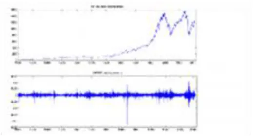
The complexity of financial time series is exhibited on the figures below. On the first figure we present historic data of the prices of an individual stock, namely IBM stock prices in the period of 1991-2011.
In the second figure we present historic data of the prices of an index, representing the overall dynamics of a collection of stock prices, namely the NASDAQ index values in the period of 1991-2011:
These models are called technical models, as opposed to fundamental models in which the minute details of the market, in particular the behavior of the agents, are described. The advantage of using technical models is that they lead to tractable mathematical problems. In addition, simulation results show, that financial data generated using an assumed micro-structure of the market, can be superbly described, in a statistical sense, by an appropriately fitted technical model.
An early powerful alternative to the random walk model is the so-called linear model, in which the dynamics of the market with its millions of small feedback effects is reflected in the fact that we the model has a a non-zero, (but fading) memory. Linear models are quite acceptable for preprocessed data, having non-zero means, linear trends or periodic cycles removed by appropriate methods. Linear models also have a highly developed and sophisticated theory thanks to their multiple relevance in circuit theory, communication and systems and control theory, with major contribution by the R. Kalman.
Linear models are quite acceptable for preprocessed data, having non-zero means, linear trends or periodic cycles removed by appropriate methods. A neuralgic point in using a linear model is that it is completely specified by second order statistics, and finer properties of the return processes may not be reflected. In particular, within the class of linear models all second order stationary orthogonal processes (often called white noise precesses) are statistically equivalent, or indistinguishable.
To model the phenomenon of volatility clustering we would need a to consider a finer model structure in which todays returns influence tomorrows conditional volatility. On the other hand we wold like to get a model which is mathematically tractable. A breakthrough in dealing with the above problem was provided by the classical paper of Engle [14], in which the so-called ARCH (autoregressive conditional heteroscedasticity) model was introduced. The proposed application area in that paper was the analysis of macroeconomic data. Standard generalizations of ARCH models are the so-called GARCH (generalized ARCH) models, introduced by Bollerslev [4]. It turned out that GARCH models are excellent candidates for modelling financial data with exhibiting stochastic volatility.
The extraordinary attention paid to these models in the academic community is due to the fact that this a technical model defined via a relatively simple dynamics, yet leading to a variety of interesting theoretical problems, and at the same time it is versatile enough when fitting to real data. Robert Engle is the the winner of the 2003 Nobel Memorial Prize in Economic Sciences, sharing the award with Clive Granger, "for methods of analyzing economic time series with time-varying volatility (ARCH)".
Another important development in modeling financial time is the construction of high frequency (continuous time) model classes allowing to model shocks or jumps in the price process. Thus we come to model classes using so-called Lévy processes. A rough idea of the latter can be given as follows: take the limit of a so-called compound Poisson process which has a finite number of jumps in a finite interval at times the number of which follows a Poisson distribution. There are a number of models using Lévy processes to model financial time series, such as the Variance Gamma or the CGMY model. The special feature of these models is that the characteristic function rather than the distribution function of the price is known explicitly, possibly modulo a few unknown constants.
In this course we discuss selected topics of the theory of stochastic processes with special attention to areas used in modelling financial time series, as discussed above. The basic question in connection with financial time series is very simple: predict future values of financial instruments as accurately as possible to support a decision to buy or sell. While there are powerful model-free methods for prediction based on the patterns of past ups and downs, prediction theory and practice is still dominated by model-based approaches. In this setting we first try to understand the mechanism by which our data has been generated.
First we need to construct potential classes of models that may be appropriate for modeling. Finally, the properties of these models have to be understood and a theory of prediction has to be developed. Then we have to derive methods to describe real data by a single element of the proposed model class. This last step is called estimation in the mathematical statistics literature, while the terminology identification is accepted in the engineering literature.
As for the selection of the course material we should note that the development of the theory of stochastic processes was significantly inspired by telecommunication and later by systems and control theory, and the interaction between engineering and finance is not over yet.
The course is suitable for students with a solid basic training in basic probability theory and introductory functional analysis. To assist the learning process many of the smaller mathematical facts are formulated as exercises. Some of these are marked with a * to indicate that their solution may require a bit more than straightforward, one-minute application of known facts.
The solutions to these exercises are available at
http://digitus.itk.ppke.hu/~vago/Financial_Time_Series_pdf/
Moreover, course material is supplemented with a number of sophisticated interactive simulation programs available at
http://digitus.itk.ppke.hu/~vago/Financial_Time_Series/
It is hoped that experimenting with these programs will help the student to develop a feeling for the variety of behaviors of data generated by our models.
Finally, a pdf version of the course material, allowing for future corrections and updates will be available at http://digitus.itk.ppke.hu/~vago/Financial_Time_Series_pdf/
2. 1 Basic concepts
2.1. 1.1 Wide sense stationary processes
A discrete time stochastic process is simply a sequence of random variables over a fixed probability space . The subscript indicates time, the range of which is assumed to be typically for the sake of mathematical convenience. When we speak about a random variable we assume that it is real valued, unless explicitly stated otherwise. Complex valued random variables will indeed play an eminent role in our discussions. Depending on the application area a stochastic process may be called a time series (economics) or a random signal (telecommunication and control).
A key property of a stochastic process is the dependence structure between the random variables . Dependence is what makes prediction possible. Another key property of a stochastic process is a kind of statistical homogenity in time, which again makes prediction possible.
The simplest measure of dependence is covariance or correlation. Thus in most part of the course we will restrict ourselves to processes such as that
Equivalently, we have for all . Here stands for the Hilbert space of equivalence classes of real valued random variables with . In this course we will identify a class of a.e. identical random variables with a representative of its class.
To model statistical homogenity first we will assume that for some
A good measure of dependence is the covariance
Statistical time-homogenity then would mean that the above covariance is independent of . Thus we arrive at the following concept:
Definition 1.1. A real valued stochastic process , is called wide sense stationary, w.s.st. for short, if for all , and for some
and
is independent of . The function is called the autocovariance function.
Three examples of so-called AR processes (see Chapter 5) are shown below:
An alternative terminology is that is a second order stationary process or weakly stationary process.
A standard assumption will be in this course that the expectation of is for all , i.e.
Then the autocovariance function is defined as
Remark. The assumption is not restrictive. If we have a general w.s.st. process , then the process defined by will be a zero mean w.s.st. process.
Note, that the autocovariance function is symmetric, or even:
and that
If we allow to be complex valued then the above definition, restricted to the case of zero mean processes, is modified by requiring that for all , and, assuming ,
and
is independent of , where denotes the complex conjugate. For complex w.s.st. processes we have
The condition will also be expressed by saying that , the Hilbert space of complex valued random variable with . Here again we will consider identical r.v.-s which are identical a.e.
The autocovariance function of an AR -process is fairly trivial. The closest non-trivial example is the autocovariance function of a so-called AR process, two examples for which are given below:
Exercise 1.1.Let be a wide sense stationary process and let us define
Show that is also a wide sense stationary process.
Let us compute . We have
Define the matrix by
and the vector
Then we can write
The matrix is obviously symmetric and positive semi-definite. In addition, its elements are constant along any sub-diagonal:
Such a matrix is called a Toeplitz matrix.
Exercise 1.2.Set
Prove that the matrix defined under (1) can also be written as .
Exercise 1.3.Using the representation prove that is symmetric and positive semidefinite.
To sum up our findings we have:
Proposition 1.2. The matrix defined under (1) is a symmetric, positive semi-definite Toeplitz matrix.
For complex-valued processes we have a similar result:
Exercise 1.4.Let be a complex-valued w.s.st. process with auto-covariance function . Show that the matrix defined by
is a Hermitian, positive semi-definite Toeplitz matrix.
2.2. 1.2 Orthogonal processes and their transformations
How do we get a wide sense stationary process? Let us start with the simplest possible w.s.st. process called w.s.st. orthogonal process. This is a w.s.st. process characterized by
Below we plot the graph of an orthogonal process:
The last condition can be expressed in the geometry of Hilbert spaces by saying that the random variables and are orthogonal for . This explains the terminology. In terms of the autocovariance function we may say that
To summarize:
Definition 1.3. A w.s.st. process satisfying (3) is called a w.s.st. orthogonal process.
An alternative terminology is that is a white noise process.
As a practical example we mention that an often used assumption in modeling financial time series is that the return processes are identically and independently distributed, in short, they are i.i.d. They can also be assumed to have zero mean after discounting. If, in addition, they have finite second moments, then they form a w.s.st.
orthogonal process. Although it should be mentioned, that the price dynamics based on the assumption of i.i.d.
returns fails to reproduce some basic features of a real price process. In fact, daily return data from the past, called also historical data, exhibit a small correlation. In addition, the assumption on i.i.d. returns would lead to a price process the variance of which is unbounded, contradicting basic theoretical speculations. This contradiction is particularly obvious with agricultural products, the prices of which are tied to meteorological data, which are inherently bounded.
Now let us consider a practical example from engineering for a mechanism through which more general w.s.st.
processes are generated from w.s.st. orthogonal processes. Let us think of as the vertical displacement of a road surface properly normalized by its mean, measured at equidistant points not too close to each other. Then we may rightly assume that the -s are uncorrelated. Now if a car rolls along this road then the unevenness of the road surface causes the body of the car (via a damping device) to vibrate. An exact description of this effect is given in the literature on so-called half-car models. Denoting the vertical displacement of the body of the car by properly normalized by its mean, the overall picture is that is transformed into . Naive physics suggests that past values of may effect the present value of . Assuming that this transformation is linear we arrive at the following representation of :
Here the -s are the so-called impulse responses of the "system", represented by the body of the car, mapping to .
To ensure that given in (4) is well defined in some sense we resort to the Hilbert space theory. Assuming that
the right hand side of (4) converges in . Thus is well defined. To see this, for a fixed consider the random variables
Exercise 1.5.Show that the sequence is a Cauchy sequence in norm.
Indeed, for we have by the orthogonality of
if is large enough, since by assumption .
In a Hilbert space every Cauchy sequence is convergent, thus is well defined.
Exercise 1.6.Show that given in (4) is a wide sense stationary process.
The variance of is obtained as
As we shall see later the class of wide sense stationary processes given by (4) is not only an interesting instance, but actually most w.s.st. processes of practical interest fall into this class.
A special case of the above is a wide sense stationary process, which is obtained by taking a finite moving average of an orthogonal process . Thus let be a wide sense stationary orthogonal process and define
Definition 1.4.A wide sense stationary process defined by (5) is called a moving average or MA process.
If , then is called the order of the process. If we wish to emphasize the order, we say that is an MA(
) process. In engineering terminology we would say that is obtained by passing an orthogonal process through a finite impulse response (FIR) filter.
It is interesting to note that even in the simplest cases of and the visual variety of the graphs of MA processes is remarkable. In all the examples below we take . For and we take a weighted difference of the white noise process resulting in similar processes:
For and we take a weighted sum of the white noise process resulting in a kind of averaging and smoother trajectories:
For the combination of the above models results in an enhanced effect:
2.3. 1.3 Prediction
A fundamental problem of the theory of time series is the prediction of future values. In the case of a one-step ahead prediction we would like to predict for some fixed knowing past values for . In other words we assume that the complete, infinite past of up to time is known. This assumption is a matter of convenience for certain theoretical arguments.
However in practice we have to work with finite segment of data. Therefore we consider first the following problem: predict based on the finite segment of past data , , . We restrict ourselves to linear prediction of the form:
with the coefficients still to be specified. The quality of our predictor is measured by mean square error (MSE):
Minimizing with respect to yields the least squares (LSQ) predictor of within the class of linear predictors.
Obviously, is quadratic in , hence its minimization is trivial by direct arithmetic.
However, more instructive way of solving this minimization problem is to use a geometric approach.
A geometric approach to LSQ will simplify the solution of the prediction problem. Let us consider the linear space spanned by the random variables , i.e. consider all random variables of the form:
Let us denote this linear space by , or, if we want to stress the dependence on , write . Since is a wide sense stationary process and thus for all , is a finite dimensional subspace of equipped with a scalar product:
From now on, will denote the space above equipped with the scalar product inherited from . Thus is a Euclidean space. The problem of best linear prediction is then equivalent to the following geometric problem: find the orthogonal projection of on the subspace .
We will use the following notations: if is a Hilbert space and is a subspace of (i.e. a linear subspace of which is closed), then for the projection of onto will be denoted by
The projection is uniquely defined by the following two properties:
The existence and uniqueness of such a projection is a fundamental result of the Hilbert-space theory. In the case of Euclidean spaces we refer to basic linear algebra.
The best linear predictor of in terms of is then uniquely defined by the orthogonal properties:
This can be written equivalently as
Substituting (6) for and working out the left hand side we get
Introducing the notation
the right hand side becomes simply . Thus the above equation becomes
and we arrive at the following result:
Proposition 1.5. Assume that is nonsingular. Then the LSQ linear predictor of in terms of is uniquely defined as
where is the solution of
We shall discuss prediction in more detail in Chapter 5. Here we present only two graphs of two AR( ) processes and their predictor, marked yellow:
Remark. The coefficients of the best linear predictor are uniquely determined if is nonsingular, or equivalently, if is positive definit. What if is singular? Then we have a non-zero vector such that
which is equivalent to writing that
Exercise 1.7.Show that if is singular then can be predicted with error.
We would not want to consider stochastic processes which can be predicted with error as truly random. We shall therefore single out such processes with the name "singular processes". For details see below.
We conclude this section with two non-trivial exercises:
Exercise 1.8. Show that for the process we have
Exercise 1.9. Show that
3. 2 Prediction, innovation and the Wold
decomposition
3.1. 2.1 Prediction using the infinite past
Let us now consider the prediction problem with . Predicting using infinite past looks impractical at first. However, it provides us with a fundamental insight into the structure of the process, Moreover, as we shall see, it can often be realized by a finite recursion. To formulate the problem, we need a little more care. Define the linear space
Obviously
The closure of in is a subspace of which will be denoted by . Formally we write
Thus consists of all random variables that can be approximated arbitrarily well in -sense by linear combinations of the form
Then the best linear predictor of in terms of infinite past is defined as
A key object in the theory of wide sense stationary processes is the prediction error
Loosely speaking the random variable expresses the information content of not contained in when we restrict ourselves to linear approximations.
Definition 2.1.The process
is called the innovation process of . Exercise 2.1.Prove that
Proposition 2.2. is a wide sense stationary orthogonal process.
Proof.Obviously
is a wide sense stationary process. (Why?) Taking limit we get, that is wide sense stationary. The orthogonality of is obvious. [QED]
Processes with the property that a finite segment of past values is sufficient to compute the best linear predictor are of particular interest. If is such a process then we can write
where is the innovation process of .
Definition 2.3. A wide-sense stationary process satisfying (7) is called an autoregressive or AR process.
If , then is called the order of the process. If we wish to emphasize the order, we say that is an AR(
) process.
3.2. 2.2 Singular processes
A "truly random" process has a non-trivial innovation, i.e. . Thus in a strict sense. A process with zero innovation would thus be an anomaly. For such a process we would have
Exercise 2.2.Show that if for a single , then for all . Definition 2.4.A process is singular, if
holds for all .
It follows that can be arbitrarily accurately approximated by linear combinations of the form in the sense. The question arises: "How we can construct such a process?"
Consider the complex-valued process:
where is a fixed frequency, is an eventually complex-valued random variable with
Exercise 2.3.Show that the above process is wide sense stationary:
and
is independent of .
Note that the autocovariance function does not decay in absolute value, as increases, indicating a strong dependence between past and present.
The above process is not "truly random" in the sense that two values of , say and , uniquely determine the (random value of) and , and thus the complete future of is known. Formally, we are tempted to assume that is obtained from . But thus would be a non-linear(!) function of . In spite of this, our intuition is right.
Exercise 2.4.Show that is singular, i.e.
A simple proof is obtained by applying the result given in the following exercise:
Exercise 2.5. Let be a w.s.st. process such that for some . Then is singular.
Consider now a finite sum of complex-valued singular processes of the form
where for . Assume that
In addition, assume that the random coefficients are mutually orthogonal, i.e.
The last condition is crucial in proving the following result:
Proposition 2.5. The process defined by (8) is a wide sense stationary process.
Proof.Obviously we have for all . The autocovariance function for
is indeed independent of . [QED]
Exercise 2.6.Prove that the process defined above by (8) is singular, i.e.
(Hint: Apply previous Exercise.)
The variance of is obtained by setting :
We conclude, that the contribution of the frequency to the variance of is . In telecommunication is the energy of the random signal. Correspondingly, the values show how the energy of is spread along different frequencies.
This simple and to some extent artificial construction of a wide sense stationary process can be significantly extended. In fact, we will see that by an appropriate extension of the representation given in (8) we can recover any wide sense stationary process. Needless to say that in such an extension the anomaly of singularity may disappear.
Remark. It would be wrong to believe that all singular processes are of the form given in (8). There are examples for singular processes, where singularity can not be established by direct inspection.
A simple example for a real-valued singular process is given by
where is a random phase with uniform distribution on .
Exercise 2.7.Show that is a wide sense stationary process.
Exercise 2.8.Show that is singular. (Hint: Apply the identity
).
3.3. 2.3 Wold decomposition
Let us now consider a process which is not singular, i.e.
in a strict sense, or equivalently, its innovation process
is not zero. We have seen that is a wide sense stationary orthogonal process. Write
Now decompose the second term as
where . Note that any random variable such that and can be
written as
with some real . (Why?). Then we can write
Continuing this argument we get
with The question now arises, how to deal with the residual term.
Let us define the Hilbert space of distant past, or prehistory of as
Lemma 2.6. For any random variable we have
Exercise 2.9. Prove Lemma 2.6
To prove Lemma 2.6, we first formulate a dual result:
Lemma 2.7.Let be a monotone increasing sequences of Hilbert subspaces, i.e.
. Let
with denoting the closure. Then for any we have
Exercise 2.10. Prove Lemma 2.7.
Define
and
with the limit interpreted in . Then we arrive at the following decomposition of :
Exercise 2.11.Show that the processes and are orthogonal, , meaning that
(Hint. Note that for any and any we have )
Exercise 2.12.Show that for the process we have
(Hint: First show that for all , then show that The latter follows from the fact that for all )
Definition 2.8.A process is called completely regular if
Proposition 2.9. The process defined under (9) is singular and
Proof.First we show that the infinite past of the off-spring process is contained in the the infinite past of , i.e.
To see this, note that the definition implies for all , which in turn implies for all But then the representation of as a linear combination of past values of implies
and hence for we also have
We conclude from here that
which implies as stated. [QED]
Now to prove the opposite inclusion, note that the decomposition of as with implies
for all , where denotes orthogonal direct sum. Now formally taking intersection over , and using the fact that would give the result. This formal argument can be elaborated as follows. Let . Then for all . Let us write as
with and . Then
Now letting tend to infinity we get that
by Lemma 2.6. But , hence and we conclude that
Obviously, the right hand side belongs to for all and hence it belongs to .
Thus we arrive to the following result, which is known as the Wold decomposition of a w.s.st. process:
Proposition 2.10.Any wide sense stationary process can be decomposed as
where is completely regular, is singular and . Moreover
The singular component of the process contains a priori randomness, or randomness in the distant past or prehistory of .
To complete the above result, consider now a completely regular process . By the construction of we have On the other hand the representation
implies Thus we arrive at the following result.
Proposition 2.11.Let be the innovation process of a completely regular process . Then
with and
4. 3 Spectral theory, I.
4.1. 3.1 The need for a spectral theory
Let us revisit the problem of prediction. Let be a completely regular stochastic process that can be written in the form
where , and is the innovation process of . Then the LSQ predictor of is given by
By this the problem of prediction seems to be solved. But in fact this is not the case: we would like to express in terms of rather than in terms of the (unobserved) .
Let us simplify the problem and assume that the representation of is actually an MA( ) process:
A useful tool for future calculation is the backward shift operator acting on doubly infinite sequences as follows:
Introducing a polynomial of as
the defining equation for the MA process above can be rewritten as
Similarly, the process formed of the one-step ahead predictors can be defined via
To express via a formal procedure, often adapted in the engineering literature, is to invert (10) as
To see if a meaning can be given to this step it is best to see an example. Let
Then
and iterating this equation we get, assuming ,
Exercise 3.1.Show that the right hand side above is well defined.
However, the situation becomes much more complicated for higher order MA models, so the interpretation of the operator needs extra care.
To find an appropriate interpretation to our formal procedure let us make a brief excursion to the theory of linear time invariant (LTI) systems. A linear time invariant system is defined by
Here is the input process, is the output process, and the coefficients are called impulse responses of the linear system. A standard tool for studying the linear time invariant systems is the so-called z-transform. Briefly speaking, consider a linear system such that
Consider a deterministic and bounded input signal . Then, as it is easily seen, the output signal will also be bounded. Define
with . Then we have the very simple multiplicative description of our linear time invariant system as follows:
To extend this ingenious device to two sided processes we run into the problem of choosing the range for . Neither , nor would do. The only option, with a vague hope of success is to try . Thus we are led to the study of a formal object of the form
The ultimate objective of spectral theory of w.s.st. processes is to give a meaning to this formal object.
4.2. 3.2 Fourier methods for w.s.st. processes
Obviously, the infinite sum above is unlikely to converge in any reasonable sense. To see how a meaning can be given, consider our benchmark example for a singular process given as
A natural first alternative to the infinite sum above is a finite sum appropriately weighted:
Proposition 3.1. We have
in the sense of and also w.p.1.
Exercise 3.2.Prove Proposition 3.1.
Corollary 3.2.The spectral weights can be obtained as
Exercise 3.3.Prove the above corollary.
This follows simply from the fact that in . Now the question arises, whether the above arguments can be extended to general processes.
Let us consider a general wide sense stationary process . We can ask ourselves: does the finite, normalized Fourier series
have a limit in any sense? For a start we can ask a simpler question: does the sequence
have a limit? Forgetting about the normalization by and expanding the above expression we can express the above expectation as
Indeed, the value of depends only on , and the number of occurrences of is . (To double-check this note that the number of occurrences of is , while the number of occurrences of is .)
Now at this point we shall make the assumption that
This assumption would then enable us to apply Fourier theory. (Note, however, that with this assumption our benchmark examples for singular process are excluded!) Now, the right hand side of (13) can be related to the partial sums of the Fourier series of as follows. Defining
we can write the r.h.s. of (13) as
Now assumption (14) implies that
is well-defined in the sense that the right hand side converges in , where stands for the standard Lebesgue-measure. It follows by the celebrated Fejérs theorem that the Fourier series of
also converges in the Cesaro sense a.s., i.e.
Thus we come to the following conclusion.
Proposition 3.3. Under condition (14)
exists a.s. on w.r.t. the Lebesgue-measure, and we have
where the r.h.s. converges in and also in Cesaro sense a.s. with respect to the Lebesgue-measure.
4.3. 3.3 Herglotzs theorem
From Proposition 3.3 immediately get a special form of the celebrated Herglotzs theorem:
Proposition 3.4.Under condition (14) we have
with some , . In particular
A remarkable fact is that the latter proposition, in a slightly modified form, is true for any autocovariance sequence. More exactly we have the following result:
Proposition 3.5.(Herglotzs theorem) Let be the autocovariance function of a wide sense stationary process.
Then we have
where is a nondecreasing, left-continuous function with finite increment on , with . We have
in particular.
The function is called the spectral distribution function, and the corresponding measure is the spectral measure. The integral above can be interpreted as a Riemann-Stieltjes integral. The distribution function is like a probability distribution function except that we may have .
Remark. At this point we need to recall that there is a dichotomy in defining a probability distribution function.
If is a random variable then its distribution function may be defined either as or , depending on local traditions. In the former case is continuous from left, in the latter case is continuous from right. In this lecture we will assume that is left-continuous. Thus the measure assigned to an interval is . Let us now see the proof of Herglotzs theorem.
Proof.Let us truncate the autocovariance sequence by setting
Exercise 3.4.Show that the truncated sequence itself is an auto-covariance sequence.
Obviously, is a positive semi-definite sequence. Hence it is an auto-covariance sequence.
Then we have by the special form of Herglotzs theorem that
with . Defining by
we have
Obviously is nondecreasing for all . Now we have
Now we can refer ro Hellys theorem stating that there exists a subsequence and a monotone nondecreasing function such that
at all continuity point of , and . This is also expressed as saying that converges to weakly, or formally writing:
It then follows by classical results of introductory probability theory that for every bounded continuous function we have
For in particular we have for any fixed
Q.e.d. [QED]
4.4. 3.4 Effect of linear filters
To see the power of Herglotzs theorem, we present the following simple result:
Proposition 3.6. Let be a wide sense stationary process. Then for any finite linear combination
we have
where
Exercise 3.5.Prove the above proposition.
To extend the above result, the question can be raised: how we can conveniently express the auto-covariance function of the process
obtained from by applying a finite impulse response (FIR) filter. Or in other terms: how do we get the spectral distribution of from that of ?
Note that we have:
Now expressing via Herglotzs theorem we get, after interchanging the sum and the integrand,
Introducing
we come to the following conclusion:
Proposition 3.7. For the spectral distribution of the process we have
If has a spectral density then also has a spectral density and we have
The complex valued function is called the transfer function or frequency response function of the FIR filter. If than the energy contained at frequency will be amplified, for it will
be attenuated. For appropriately chosen weights the filter may be such that is close to zero except for a small band around a specific frequency . An ideal case would be when
and otherwise. Such a filter is called band-pass filter. It is readily seen that such a filter can not be represented as an FIR filter. (Why?)
5. 4 Spectral theory, II.
5.1. 4.1 First construction of the spectral representation measure
Let us now return to the Fourier transform of the series of itself:
At this point assume that
Let the spectral density of be denoted by We can not expect that the Fourier transform of will converge in any reasonable sense (unless ). On the other hand, if then, using a heuristics that can be made precise, is the inverse Fourier transform of the Dirac delta function assigning a unit mass at the point . Hence the Fourier transform of itself is the the Dirac delta function. While the Dirac delta function is a generalized function, its integral is an ordinary function (namely the unit step function). These observations motivate us to consider the integrated process
We can write
Note that can be interpreted as the Fourier coefficients of the characteristic function of the interval , which we denote by .
Let us now compute . We have
where
Write as
Now the latter sum is the Fourier series of the characteristic function . Thus
in . Since is an element of and the scalar product in is continuous in its variables, we conclude from (17) that
By similar arguments we can see that if we now look at the increments of on two non-overlapping intervals and contained in then we get
Using the same train of thought it is easily seen that is a Cauchy sequence in , hence it converges to some element of denoted by :
Furthermore, if we take two non overlapping intervals and then we have
We will express this fact by saying that is a process of orthogonal increments. To summarize our findings:
Theorem 4.1. Let be a w.s.st. process with autocovariance function such that
Then
in , where is a process with orthogonal increments. Moreover, denoting the spectral distribution function of by we have
5.2. 4.2 Random orthogonal measures. Integration
The question is now raised: how we can represent a general wide sense stationary process as an integral of weighted trigonometric functions in the form
where is a random weight defined as some kind of random measure. Thus is a substitute for the
random coefficients appearing in the definition of singular processes of the form . Recalling the conditions imposed on we define "orthogonal random measures " via the stochastic processes of orthogonal increments. The definition of the latter is obvious, it is almost a tautology:
Definition 4.1.A complex valued stochastic process in is called a process with orthogonal increments, if it is left continuous, , for all , and for any two non-overlapping intervals and contained in we have
The "measure " assigning the value to an interval is called a random orthogonal measure. The function is called the structure function. It is assumed that is left continuous.
From the definition it follows that
Exercise 4.1. Prove, that for any we have
thus is monotone nondecreasing.
(Hint: Write as the union of and and apply Pythagoras theorem.)
Let now be a random orthogonal measure on , and let be a possibly complex valued step function of the form
where is a finite set, and the intervals are non-overlapping. Then define
Thus is a random variable which is obviously in , where indicates that we consider the space of complex valued functions.
Exercise 4.2.Let , be two left continuous step functions on . Then
(Hint: Take a common subdivision for and .)
Let be the set of complex-valued left-continuous step-functions on . Obviously is a linear space and . Thus (18) can be restated saying that stochastic integration as a linear operator
is an isometry.
Exercise 4.3.Prove that
is w.s.st.
5.3. 4.3 Representation of a wide sense stationary process
Perhaps the most powerful tool in the theory of w.s.st. processes is the following spectral representation theorem, which will be used over and over again in this course.
Theorem 4.2. Let be a wide sense stationary process. Then there exists a unique random orthogonal measure , such that
The process is called the spectral representation process of .
Proof.Assuming that can be represented as stated we have
Thus the structure function of is necessarily determined by the spectral distribution of , denoted by , as follows:
Now, integration with respect to defines an isometry from into
. Conversely, if such an isometry is given, then it defines an orthogonal random measure on with structure function simply by setting
Thus finding the spectral representation process is equivalent to finding the isometry from
into .
Now, the assumed representation for implies the following specifications for :
From here we could argue as follows: to get write
where convergence on the right hand side is assumed to take place in . Then, by the continuity of , we would get
The difficulty with this argument is to actually find the representation of as given under (20), when convergence of the right hand side is required in a possibly strange norm defining . Therefore we follow another line of thought. Consider the set of specifications (19) prescribed for . Let us now extend the definition of the yet undefined isometry to the linear space
Define for
Consider as a linear subspace of . The linear extension of is well-defined if is independent of the representation of . This is equivalent to saying that in implies
Exercise 4.4.The above implication.
[QED]
The last argument also shows that is an isometry from to . Since is a dense linear subspace in , can be extended to a linear isometry mapping from into in a unique manner. As said above, the orthogonal random measure itself is obtained by setting
Exercise 4.5.Show that the structure function of the random orthogonal measure is , predetermined by the spectral distribution function of .
Let now denote the isometry from to defined by integration w.r.t. :
Then and agree on all characteristic functions , and therefore and agree on all step functions.
Since the latter are dense in , we conclude that . It follows, that
as stated.
5.4. 4.4 Change of measure
Let be a random orthogonal measure on with the structure function . Let , and define
Exercise 4.6.Show that is a random orthogonal measure, with the structure function
The corresponding random orthogonal measure will be written as
Let now be a function in . Note that we have taken an element of a new Hilbert-space, defined by . Then
is well-defined. Now we have the following, intuitively obvious-looking result:
Proposition 4.2. We have
Proof.The proposition is obviously true if is a characteristic function . Since both sides of the stated equality are linear in , it follows that the proposition is true whenever is a step function. Now let be an arbitrary function in and let be a sequence of step functions converging to in the corresponding Hilbert-space norm. Then
On the other hand, the assumed convergence
implies
But then, the isometry property of stochastic integral w.r.t. gives
and the proposition follows. [QED]
5.5. 4.5 Linear filters
Let us now consider the effect of linear filters on the spectral representation process. Let be a wide sense stationary process with spectral representation process . Define the process via a FIR filter as
Then is a wide sense stationary process.
Exercise 4.7.Show that the spectral representation process of is given by
where
Let us now consider the infinite linear combination
We have seen that the r.h.s is well defined (converges in ), if the infinite series
is well defined in .
Proposition 4.3.The spectral representation process of is given by
Proof. Truncate the infinite sum defining at , i.e. define
Then the spectral representation of is given as
where
Now letting tend to infinity, the l.h.s. of (21) converges to in .
Exercise 4.8.Show that the integrand on the right hand side converges to in
Thus the corresponding integral w.r.t. will converge to
in . This proves the claim. [QED]
6. 5 AR, MA and ARMA processes
6.1. 5.1 Autoregressive processes
Consider now a process that is implicitly defined via the equation
where is a w.s.st. orthogonal process.
A shorthand notation is
where is the backward shift operator, and
Proposition 5.1. Assuming that for all , the equation (23) has a unique wide sense stationary solution . The process has a spectral density equal to
Proof.Assume that a wide sense stationary solution exists. Let the spectral distribution process of and be denoted by and , respectively. Then
from which we get formally
Recall, that the spectral density function of is
If for all , then is in , where is the spectral measure of , modulo a constant multiplier. Indeed, we have
where is the complex unit circle and is continuous on , thus the line integral is well defined.
Hence the right hand side of (24), as a new random orthogonal measure, is well defined. It follows, that the wide sense stationary process
is well defined. If there is a solution, then it must be equal to the process just defined. By this uniqueness is proved. On the other hand, it is easily seen that the process is indeed a solution of (22). Namely,
This proves the existence of a solution, and the proposition is proved. [QED]
The graphs of a two newly selected AR processes are shown on the figures below together with their autocovariance functions:
More complex behaviors can be noticed on the graphs of AR( ) processes below:
The above derivation demonstrates the supreme power of spectral representation: the outline of the proof is easily obtained by formal arguments, which then are easily filled with rigorous technical details. It is not clear at this point if there is any other more direct method that would yield the proposition. An exception is the case
, but even there we may run into unexpected challenges.
6.2. 5.2 A classic result: the Yule-Walker equations
AR processes are of particular interest due to the fact that a finite segment of its past values is sufficient to compute the best linear one-step ahead predictor. Let be a stable AR( ) process, satisfying
where is the innovation process of . Recall that if then is called the order of the process.
The question can be put: how the auto-covariances of say are to be computed.
Let and multiply equation (25) by Taking expectation, and using the that we get the following system of linear equations:
We have linear equation for the first auto-covariances. This set of equations is called Yule - Walker equations. The coefficient matrix of this systems of linear equations is
This is a so-called circulant matrix the eigenvalues of which are known to be of the form where Now if on the no eigenvalues are hence the Yule-Walker equation has a unique solution. Recall, that in Proposition 5.1 this was the condition for the unique wide sense stationary solution of the AR process. Thus the first auto-covariances are uniquely determined.
For the auto-covariance can be computed recursively in terms of previous values of using the same arguments as above: multiplying equation (25) by and taking expectation we get
Special case. For the Yule-Walker equations consist of two equations:
The solution is well-known:
and further on for .
6.3. 5.3 The AR process
Thus let us now consider an AR( ) process defined by
Let us first assume that . Recall the examples below from Chpater 1:
Then for , and by the above theorem a unique solution exists. The existence and uniqueness of the solution can directly be seen as follows. First assume that a w.s.st. solution exists. Then iterating (26) we get after steps
The residual term tends to for in , thus we get
It is easy to see that the right hand side is indeed convergent in for . This proves uniqueness. It is also easy to see that the process defined by (27) is indeed a solution of (26), proving existence.
Exercise 5.1.Prove that defined by (27) does indeed satisfy (26).
Equations (26) and (27) also imply that and and thus
It follows that is the innovation process of .
Let us now consider an AR( ) process defined by (26) with . Then, again,
for , thus a unique solution of (26) exists. However, iterating (26) as above does not yield a representation of the form (27). Nevertheless, if we rewrite (26) in the form
and iterate this equation forward in time we get that must be of the form
Exercise 5.2.Show that the r.h.s. is well-defined, and does indeed satisfy (26).
Thus is expressed via the future of the wide sense stationary orthogonal process . Therefore we conclude that
and thus is not the innovation process of .
6.4. 5.4 Stable AR systems
Let us now consider a higher order AR process defined by
with deg . We can ask ourselves: under what conditions is the innovation process of .
Obviously, a backward iteration of (28), that worked nicely for , is not easily manageable. Hence we will settle the issue within the framework of spectral representation. Obviously, we have as before. To prove the opposite inclusion, , we need to express in terms of the past of . This will be certainly possible, if the rational function can be expanded into a power series of The possibility of such an expansion is clearly related to the position of the zeros of .
Definition 5.2.A polynomial of , with is called stable if
Lemma 5.3.If is a stable polynomial with then
where convergence on the right hand side is uniform in .
It follows immediately that the r.h.s converges also in .
Proof.Consider the function with taking its values in . The equation has, counted with multiplicity, exactly roots. Hence, the stability of implies that is analytic in
with some , or equivalently, analytic in for with some
. Therefore it can be expanded into a Taylor series of around
which is convergent uniformly for with some . It follows that (29) converges uniformly for . Finally, follows by evaluating the two sides of (29) for . [QED]
Let us now consider the AR( ) process defined by
where is a wide sense stationary orthogonal process, and is a polynomial of with
and .
Proposition 5.4. If the polynomial is stable then is the innovation process of .
Proof.Obviously , thus we need only to prove that . Now
Thus
Since the infinite series on the right hand side (multiplicated by ) converges in , we can interchange the integration and the summation to get
[QED]
Remark. The converse result also holds: if is a polynomial with for and the AR(
) process defined by (30) has for its innovation process, then is stable.
6.5. 5.5 MA processes
A simple class of wide sense stationary processes is obtained by taking a finite moving average of an orthogonal process . Thus let be a wide sense stationary orthogonal process and define
Exercise 5.3.Show that is a wide sense stationary process.
Definition 5.5.A wide sense stationary process defined by (31) is called a moving average (MA) process, or more precisely MA( ) process.
In addition to the examples given in Chapter 1 the graphs of a simulated MA process are displayed below:
In engineering terminology we would say that is obtained by passing an orthogonal process through a finite impulse response (FIR) filter.
The autocovariance function of this process can be computed as follows:
Thus the coefficients uniquely determine autocovariances . In the other direction uniqueness is not true. We show a simple example.
Example. Consider the w.s.st. processes:
Assume , then the two processes are different. Nevertheless, their autocovariances are the same, we have
Rearrange (32) to get and iterate this equation. We get the following formal series
Similarly, from equation (33) we get
We get two formal infinite series reconstruction of . A process is called invertible if the reconstruction of is possible. In this example it is equivalent with the convergence of the formal infinite series.
Exercise 5.4.Show that (34) is well-defined, if , i.e. . Similarly, (35) is well-defined if .
Hence, although the autocovariances of both processes are the same, only one of them is invertible, depending on the value of .
6.6. 5.6 ARMA processes
Let us now consider the combination of AR and MA processes.
Definition 5.6. A wide sense stationary process is called an ARMA process if it satisfies the difference equation
where is a w.s.st. orthogonal process, and , are polynomials of the backward shift operator . The degrees and of and , respectively, are called the orders of the ARMA process.
Writing
we assume that . If the degrees of and are and , respectively, then also and If we want to stress the orders we say that is an ARMA( ) process.
The graphs of simulated ARMA processes together with their auto-covariance functions are displayed on the figures below:
Straightforward extensions of Propositions 5.1 and 5.4 are the following results:
Proposition 5.7. Assume that for . Then there is a unique w.s.st. process satisfying (36).
Exercise 5.5.Prove the above proposition.
Proposition 5.8. Assume that and are stable polynomials. Then is the innovation process
of .
Exercise 5.6.Prove the above proposition.
6.7. 5.7 Prediction
Now we have all the machinery to revisit the prediction problem in general, and for ARMA processes in particular. Let be a completely regular w.s.st. process with innovation process . Then we can write
with . The one-step ahead predictor of is then given by
Here we have taken into account that , and hence
To complete the above argument we have to express in term of . This can be done best in the spectral domain. Let us write (37) in the form
Then
Note that the right hand side is well defined, since , we have
. The one-step ahead predictor given by (38) can be described by
Combining (39) and (40) we get the following result:
Proposition 5.9. Let be a completely regular wide sense stationary process given by (37). Then its one step ahead predictor is obtained via the spectral representation measure
The above result provides a general solution to the prediction problem for regular processes. A shortcoming of this result that it is formulated in the spectral domain.
It is important to stress that may not be written as an infinite series which is convergent in . In other words, a linear filter in frequency domain (amounting to re-weighting the frequencies) does not necessarily have a time domain representation. However, the situation is simplified considerably in the case of ARMA processes.
Let be a wide sense stationary ARMA process defined by
where and are stable polynomials. Then is the innovation process of , and setting
we can write (41) as
The stability of implies that
where the right hand side converges in . Applying Proposition 5.9 we get
Multiplying both sides by and converting the resulting equality to time domain we get the following result:
Proposition 5.10. Let be a wide sense stationary ARMA process given by (41), where and are stable. Then the one-step ahead prediction process is defined by the equation
Note that implies that the constant term of is , and hence the result of its action on at any time can be computed using only values of up to time . Thus we do get a genuine one-step ahead predictor.
The prediction of three ARMA processes, using AR(4) approximation, are displayed below. The predicted processes are displayed in yellow.
In dealing with actual data prediction is based on models based on the data, therefore the exact true dynamics is unknown. It is therefore an interesting experiment is to see the effect of parametric uncertainty onto prediction.
In the figures below we display three AR(4)-processes together with their predictors based on artificially and randomly perturbed models. It is interesting to note that these misspecified predictors perform remarkably well:
6.8. 5.8 ARMA processes with unstable zeros
Let us now consider the problem of predicting an ARMA process when not necessarily stable.
An innocent looking example is
with . The obvious thing to do is to find an alternative representation of in terms of its innovation process, which we denote by . To see how this can be done we consider a general MA process given by
where is a polynomial of and is a w.s.st. orthogonal process. Assuming the spectral density of is then given by
This can also be obtained by restricting the complex-function
to , since the coefficients of are assumed to be real. Let us now assume that has an unstable root, say . Then factorizing we will have a factor of the form
The effect of this factor in is
Thus the zeros of the above rational function are and . It is now clear that we can swap the role of and without changing the function (43). Indeed, setting
we have
The main benefit of this transformation is that the (first order) polynomial is now stable. Replacing all factors of by stable ones we come to the following conclusion.
Proposition 5.11. Let be a polynomial such that for . Then a stable
polynomial with such that
The decomposition of the spectral density of in the form given by the r.h.s. of (44) is called spectral factorization, and is called a stable spectral factor. Setting we get a factorization of the spectral density of , denoted by , as
Now, to find the innovation process of , we will not invert (42), but rather define a new process by
It is readily seen that the r.h.s. is well defined since is in . Moreover the spectral density of is
Thus is a w.s.st. orthogonal process. Since
with stable, is the innovation process of . To summarize we obtained the following result:
Proposition 5.12. Let be an MA process given in (42). Assume that for . Let be the stable spectral factor of , and define by (45). Then is a w.s.st. orthogonal process,
and is the innovation process of .
The above procedure can be extended to ARMA processes in a straightforward manner. Let be a w.s.st.
ARMA process given by
where the polynomials and are not necessarily stable, but and
for , and the process is a w.s.st. orthogonal process with . The spectral density of is then given by
Let and be the stable spectral factors of the denominator and the numerator, respectively.
Then
The rational function is called a stable spectral factor of . Now define the w.s.st. process by
Note that the transfer function
is such that
for all . A transfer function satisfying (46) is called all-pass, indicating that all frequencies are passed through the filter corresponding to with unchanged energy.
It is readily seen that the new process is a w.s.st. orthogonal process. This is formally and generally stated in the next exercise.
Exercise 5.7.Let be an all-pass transfer function, and let be a w.s.st. orthogonal process. Then the process defined by
is also a w.s.st. orthogonal process.
The simplest example for an all-pass function was obtained above in factoring the spectral density of a MA process. This is obtained by taking a first order polynomial , and swapping its zero
for , to get . Then
is all-pass.
Remark. Our result on the spectral factorization of does not cover the case when for some . Consider e.g. the process
where now , and thus . To reconstruct from we consider the corresponding spectral representation yielding
The r.h.s. is well defined in frequency domain. To get a time domain representation of in terms of consider the approximating process defined by
with . It is easy to see that
in , and also
in . It follows that
Thus , and it follows that is the innovation process of . In particular, the one-step ahead predictor of is given by