Journal of Futures Studies, June 2015, 19(4): 31-50
Erzsébet Nováky
Corvinus University of Budapest Hungary
Miklós Orosz
Tata Consultancy Services Hungary
Chaos Theory and Socio-Economic Renewal in Hungary
We utilised methods of chaos theory that were originally used in a 1990’s study to analyse the behaviour of various Hungarian socio-economic macro indicators, both historically and their expected behaviour in the future. In this study, we present the method adapted to PC and the behaviour of the selected macro indicators. We characterize the pathways our society and economy has experienced and where they are heading to into the future by the means of these indicators. Comparing the present results of analysis with the results twenty years ago (when today’s present was the future) we came to the conclusion that most of the indicators became less chaotic, thus the socio-economic courses were getting more stable over the past two decades. We conclude that the opportunity to change them is slowly diminishing, it will be more and more difficult to renew the Hungarian socio-economic indicators, and to turn the processes to more desirable courses. Recommendations for change interventions are then provided.
Chaos theory, futures studies, behaviour of macro indicators, socio-economic renewal, Hungary
Introduction
The researchers of the Futures Studies Department at Corvinus University of Budapest were studying the phenomena of chaos through futures studies in the early 1990’s, and they analysed the behaviour of a few significant Hungarian social and economic macro indicators.1 By the means of those indicators, they wanted to know whether the society and the economy of Hungary had been in the state of chaos – in its mathematical term – in those decades. They also wanted to know what the expectancies were in the future.
The time is right to take the same question into consideration again, to analyse the same
32
indicators as those selected formerly, and see what they show us now, compared to the results and forecasting from two decades back.2 We used the means provided by chaos theory for the analysis again, because they allow us to determine how much each macro indicator tends to behave chaotically, they help us to construct some possible future alternatives; and, they enable us to find out what preconditions are required for each future-alternative to become reality. Chaos theory allows us to model and analyse the course of systems that were not possible by former methods in futures studies (e.g. traditional mathematical statistics or methods based on interviewing experts collectively). It also has its limitations: it only allows managing complex systems, if their evolution can be defined by differential or difference equations, and they have regular, ordinary parameters.
Chaotic systems are dynamic systems of a few component elements with nonlinear relations between them, thus their behaviour is defined by nonlinear differential or difference equations – this is crucial for a system to behave chaotically.
Chaotic systems are extremely sensitive to initial conditions, thus a small change in the initial conditions may result in a significant change in the overall state of the system. Since they are deterministic, their future states can be calculated in principle – however their sensitivity and the error component that grows exponentially makes it impossible in practice. We separate weakly and strongly chaotic systems. For weakly chaotic systems the distance of the trajectories is growing along a parabolic curve. These systems don’t get chaotic, they are only on the verge of chaos, altering their state from one meta-stable state into another one. The trajectories of a strongly chaotic system are drawing away with an exponentially growing distance, so these systems are chaotic in its mathematical term.
The sensitivity to initial conditions – or the pace of the trajectories moving away from each other – can be calculated numerically. The Ljapunov-exponent is the logarithm of the average growth of the distance between two trajectories started from two different points in the phase space. Let’s denote the initial distance of the trajectories as δx, the number of iterations as n, the Ljapunov-exponent as λ. The estimated, maximum distance of the trajectories after n iterations – denoted by ∆x – can be calculated with the formula:
∆x = δx∙eλ∙n
If λ > 0, the behaviour is chaotic, otherwise it is not. The greater the Ljapunov- exponent is, the more chaotic the behaviour of the dynamic system is. If λ < 0, though the system is not chaotic, the closer λ is to 0, the more the system tends to behave chaotically.
We based our modelling of systems upon the critical assumption that they endeavour to grow, however they are only provided limited supplies to do so.
In nature, in our society or in our economy we can observe quite a number of phenomena supporting this assumption. We aim to describe the dynamics of restrained growth by the means of the logistic map that reflects both the urge of the system to grow exponentially and at the same time the consumption of resources at a pace the same as that of the growth. Thus, our model is a dynamical system with one variable and one parameter.
33
Analysing the social and economic indicators by the means of computer simulations
The chosen indicators
In our research conducted in 2014, we aimed to select such indicators that a relatively long time series were available for, and reflect the overall economic and social changes of the country well.3
We analysed the population, live births and deaths out of demographic indicators. The socio-economic indicators selected for our analysis were the index of the gross and net domestic product, furthermore the indicators characterizing the employment (the economically active population, the number of active earners in the branches of the economy), the production (with special attention to the indicators related to the electricity production), the investments and construction industry, the real income and consumption, the different levels of education, the availability and state of healthcare, and the tourism (number of tourists and the commercial places of accommodation). We added two more new indicators to those in our previous research that give some information on the modernization of the country.
The availability of the technologically new services can be measured, for example through the number of cellular phone and internet subscriptions. Those contain relatively short time series, but we still deemed them worth analysing.
It would have been desirable to investigate the development of the country, and how its development was sustainable – like recycling of waste, environmental costs, contamination of waters and soil, air pollution – but these are so recent and have such short time series, that their analysis by the means of chaos theory would have been too early and difficult.
The time series above are mainly from the on-line and off-line (yearbook) data provided by the Hungarian Central Statistical Office. Some time series were downloaded from the homepage of the primary source of the data.
The method of analysing the time series Chaos theory in nutshell
Chaos theory evolved from studies and analyses of dynamical systems with unexpected, seemingly random behaviour based on mathematical methods. These systems have the following common properties:
– They have deterministic behaviour defined by differential or difference equations.
– The equations that describe the behaviour of the system must be non-linear.
This is inevitable, a linear equation system never defines a chaotic dynamic system.
– They are made of a relatively few components – before the birth of chaos theory it was already known that compound systems of many components can have complex behaviour, random by appearance. However, one of the greatest achievements of chaos theory was that systems of a relatively simple structure can demonstrate unpredictable, erratic behaviour as well.
– These systems are highly sensitive to initial conditions. This means that a small modification to the initial values of the parameters of the system will result in a largely different course. To put it in another way: the distance between two paths or trajectories of a chaotic dynamical system in the phase space grows at an
34
exponential pace by time (in case of continuous systems) or by iterations (in case of discreet systems).
The systems that have the above listed features are called chaotic systems.
Since the behaviour of the chaotic systems is determined by their differential or difference equations in principal their behaviour is predictable, but it is only true for a short period. The reason is the inevitable measurement error: it is impossible to observe the exact initial value of the parameters of the system, so the distance between the path of the actual system and that of the observed system grows exponentially and soon exceed any tolerable uncertainty. When the threshold of tolerance is crossed, the behaviour will appear random. But only appear, as the behaviour is still determined by the equations, only the prediction is impossible calculated from the approximately observed initial parameters. Even though the future of a system behaving chaotically cannot be predicted, chaos theory still can help to reveal the structure of the possible future courses of the system. Chaotic behaviour is reached through a sequence of bifurcations, which we can consider as alternative futures of the system worthy for further analysis.
When it comes to the scope of the means provided by chaos theory, we must note that these are based on mathematical methods. Practically we have a system of computations, algorithms that deal with numbers, in our specific case – time series. Therefore the systems we intend to analyse by the means of chaos theory must be transformed into numbers first, and the results are also numeric. Thus, it must be possible to build a mathematical model of the system under research that describes its behaviour reliably from every important aspect. Taking all the above into consideration, the application of the means of chaos theory has the following limitations:
- its scope is limited to deterministic, closed systems;
- it analyzes relatively simple systems instead of large systems of complex sub- systems;
- the only subject of its research is the characteristics of the different states of chaos and their series;
- it can only show the transition to chaos and the possible chaotic states of those systems quantitatively by the means of its modelling methods that can be characterized by differentia or differential equations, and that have regular, ordinary parameters;
- rather long time series must be available for the mathematical means of chaos theory to produce reliable, useful results.
The algorithm explained in details
The program aiding the analysis of the time series provides a graphical support to fulfil its purpose. The program reads the selected time series, normalizes its values, thus maps them into the [0,1] interval. Next it finds the value k, for which the logistic curve generated by fL(k,x) is the nearest one to the time series read.
That is done by generating the logistic curves starting from the first value of the time series and running k from 1 to 4 incrementing it by a value desirable small (in this case 0.001). The value k found is the k of the logistic curve being the closest to the time series measured by the method of least squares. The program calculates the Ljapunov-exponent for the k found, and prints it to the console. Finally, it will
35
generate and display the graph of the selected time series, the logistic curve with the value k, and the logistic curves with some predefined k values. It also calculates those curves forward and displays them. The comparison of the graphs of the time series and logistic curves provide some help in the analysis. The k value found for the time series helps to tell if the behaviour can be seen as chaotic or not.
Now we go on analysing actual time series by the means of the algorithm described above.
The pseudo-code of the algorithm of the analysing and forecasting program:
Input parameters:
s – time series
ik – k is incremented by this value during approximation N – number of iteration we fore-calculate through Algorithms:
The time series and logistic curves are stored in arrays. If we denote an array as v, the value that belongs to ti time in the time series or in the generated curve is denoted as v[i], and v.n denotes the length of the time series.
1. Read the selected time series into the array s
2. Map the values of the time series in the array s onto [0,1] (normalize) a. Assign the largest value in s to max
b. Assign the ceiling of log10(max) to exponent c. Assign 10exponent to factor
d. Divide each element of s by factor 3. Find the k value for the array s
a. Assign ik to k
b. Fill lk with the values of the logistic curve that belongs to k i. Assign 0 to i
ii. Assign s[0] to x iii. Assign x to lk[i]
iv. Assign k×x×(1-x) to x v. Increment i by 1
vi. If i < s.n, go back to step iii), otherwise proceed to step c)
c. Calculate the distance between s and lk applying the method of least squares
i. Assign 0 to e ii. Assign 0 to i
iii. Add (s[i]-lk[i])2 to e iv. Increment i by 1
v. If i < s.n, go back to step iii), otherwise proceed to step d) d. If e<emin, assign k to kmin and assign e to emin
e. Increment k by ik
f. If k ≤ 4 then go back to step b) otherwise proceed to step g) g. Assign kmin to k
4. Calculate the Ljapunov exponent for the array s using the k value approximating a limit.
5. Append the values of forecasting to the array s applying the k value (the length of s is increased by N)
a. Assign s[s.n – 1] to x (the last value in the time series) b. Assign 0 to i
36
c. Assign x to s[s.n–1+i] (putting the values of forecasting after the last element of the time series)
d. Assign k×x×(1-x) to x e. Increment i by 1
f. If i<N, go back to step c), otherwise proceed to step 6.
6. Generate the logistic curve for k with the actual length of s (increased by N) into the array lk (like at 3b))
7. Generate the logistic curves for the values 3, 3.2, 3.4, 3.5, 3.57 with the length of s into the arrays l3,l3.2,l3.4,l3.5,l3.57 (like at 3b))
8. Display the graphs of s,lk,l3,l3.2,l3.4,l3.5,l3.57
9. END
Utilizing the result of the program
The method explained in details in the previous sub-chapter was used to investigate how chaotic the behaviour of the time series was, if any bifurcation, thus the possibility of where chaos emerged, and where the values of the actual time series were located compared to the bifurcation lines. From those properties, we infer the possible courses of processes into the future. This way we try to find the answer to the question of which processes are following a stable course in Hungary today, that are more difficult to divert to a better course, and which processes are approaching some point of bifurcation, or may be on the brink of chaos – in its mathematical term, where the possibility of more significant changes exist.
We check if a process gets close to a bifurcation point by comparing the values of the time series to the logistic curves generated using some typical k parameters by the aid of the graphs. We start the logistic map from the first value of the time series.
The typical k parameters applied are:
• k=k1=3, right on the threshold of the first bifurcation
• k=3.2, roughly the middle of the interval, where the behaviour is oscillating between two values
• k=3.4(≈k2=3.4495), a bit before where the oscillation is about to start between four values
• k=3.5(≈k3=3.5457), right before the oscillation among eight values begin
• k=3.57(≈k∞=3.5699) the onset of chaos.
We define the following categories of chaotic behaviour according to the value of k (see Nováky, Hideg, and Gáspár-Vér, 1997, p.18.):
• not chaotic, when the value of k is between 1 – 1.49
• slightly chaotic, when the value of k is between 1.5 – 2.09
• moderately chaotic, when the value of k is between 2.1 – 2.79
• strongly chaotic, when k>2.8.
In case of not chaotic systems, the bifurcation lines generated mathematically would border a wide (or very wide) range, and the curve of the actual data is running out of that range of alternatives. In case of slightly or moderately chaotic systems, the curve of the actual data is running below the bifurcation lines generated mathematically, but close to them, or it starts between the lower bifurcation lines running in the lower range and then ascends in between the upper bifurcation lines.
The curve of the actual data of the strongly chaotic systems is going between the lower and upper bifurcation lines running over the whole wide range.
The data of the past can make us come to the conclusion that, whether the future course of a certain system will keep on running out of the set of courses generated
37
mathematically (keeping their not chaotic characteristic), or whether it will run between the bifurcation lines, giving the indicator the chance of proceeding on a course better or worse than the present one. Thus, if it ascends between the upper bifurcation lines or it descends between the lower ones. The k value that belongs to the indicator shows if this change happens or not. If the value of k is greater, the indicator can be expected – by its chaotic characteristic – to move to the better, thus the upper set of courses. However it may also be – again by the chaotic behaviour of the system – that it moves to the worse, thus the lower set of courses.
It is important to mention one more aspect of analysing time series by the means of the logistic map. The reason for the behaviour of the logistic map to vary, is the fact that the growth is limited, there is a maximum the procedure can reach. This limit has a deep impact on the behaviour of the logistic map, therefore it is very important where we assume this limit during the analysis. The limit of growth is the value that is mapped to 1 when the values are mapped onto the [0,1] interval. But it is a rather complex question where the limit actually is, it can be challenging to find a suitable estimation for it. In the following analyses, we used a simple method to assume the limit by shifting the decimal point to the left, so that the largest value fits into the [0,1].
The characteristics of the chosen indicators
We have described the chosen 41 indicators with the following characteristics:
the analysed period, the k value that characterizes the course of indicators, the error that belongs to k, the width of the zone the logistic curves (i.e. bifurcation lines) spans through, the relation of the values in the time series and the bifurcation lines and the behaviour in the future.
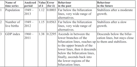
We don’t present the characteristics of every indicator analysed in our research in Table 1. Characteristics of 13 time series from the chosen for analysis, but – for the purpose of demonstration – only the characteristics of that 13 that are important from the aspect macro-economy, though their behaviour is not chaotic (like the population, the number of live births and the GDP), and additionally those indicators are shown that behave slightly, moderately or strongly chaotically for the time being.
Table 1. Characteristics of 13 time series from the chosen for analysis
Name of
time series Analysed period Value
of k Error
(for k) Behaviour
in the past Behaviour
in the future 1 Population 1949 –
2013 1.12 0.0003 Far below the bifurcation lines, very wide range of alternatives.
Stabilizes after a moderate growth.
2 Number of
live births 1949 –
2012 1.15 0.0563 Far below the bifurcation lines, very wide range of alternatives.
Stabilizes after a slow growth.
3 GDP index 1960 –
2011 1.38 0.2295 Ascends in between the lower branches of the bifurcation lines, reaches up to the upper branch of the lower lines, then it descends below the bifurcation lines, finally, ascends back into the lower regions of the bifurcation lines.
Descends below the bifur- cation lines, but stays close to them and stabilizes.
38
Name of
time series Analysed period Value
of k Error
(for k) Behaviour
in the past Behaviour
in the future 4 Volume of
investments 1960 –
2012 1.50 0.4869 Below and in the lower range of bifurcation lines ascending up to the upper part of the lower range.
Very wide range of alterna- tives.
Stabilizes at the lowest branch of the bifurcation lines after descent.
5 Number of mobile sub- scriptions
1991 –
2012 1.52 0.0481 Far below the bifurcation
lines. Stabilizes approaching the
lower bifurcation lines after a considerable ascension.
6 Number of internet subscriptions
1999 –
2012 1.54 0.0600 Starts from far below the bifurcation lines, then ascends between the lower and upper range of bifurca- tion lines at an accelerating pace.
The ascension abruptly stops and stabilizes at the lower branch of the lower range of bifurcation lines.
7 Number of deaths due to suicide, self- injury
1960 –
2012 1.56 0.3335 Below then between the lower bifurcation lines.
The range of alternatives is wide.
Stabilizes in the lower range of bifurcation lines.
8 Number of participants in secondary education
1960 –
2012 1.69 0.2828 Below the bifurcation lines, but mainly in the lower range of bifurcation lines.
Stabilizes in the lower range of bifurcation lines after a little descent.
9 Number of commercial places of accommoda- tion
1960 –
2011 1.77 3.4479 Covers almost the whole
range of its alternatives. Stabilizes in the lower range of bifurcation lines after dropping considerably.
10 Number of registered alcoholics
1980 –
2011 1.88 0.8580 Between the lower and up- per bifurcation lines, then below them.
Ascends between the lower bifurcation lines and stays there.
11 Number of economi- cally active population
1960 –
2012 1.96 0.1340 Starts from between the lower bifurcation lines, ascends between the lower and upper bifurca- tion ranges, then descends between the lower bifurca- tion branches. The range of alternatives is wide.
Stabilizes after ascending a bit.
12 Number of home units built
1960 –
2011 2.16 3.1390 Ascends between the upper bifurcation lines from the lower and upper ranges of bifurcation lines, then descends below the bifur- cation lines. The range of alternatives is wide, and is covered fully.
Ascends up to the top of the lower bifurcation lines, then stabilizes at that level.
13 Number of deaths due to cardiovascu- lar diseases
1960 –
2012 2.92 0.4218 Between the upper and lower range of bifurca- tion lines, covering a wide range.
Oscillates between the lower and upper range of bifurcation lines, about at the middle, with dropping amplitude.
Own compilation
39
None of the indicators of demography, the availability of services (telephone main stations, gross electricity consumption), indicators characterizing the general living standard (per capita real income, per capita consumption), and the indicators analysed in short term (industrial output, inflation rate, unemployment rate, change in interest rate) behaves chaotically. The k values characterizing the course of these indicators are below 1.5, they mainly run far below the bifurcation lines, and the forecasting suggests that they are going to stabilize at or close to their current level.
Thus it is difficult to change the behaviour of these indicators.
The indicators characterizing the output of the economy are a bit different. After taking a look at the time series of the GDP, it is obvious that the course of the GDP is much more changeable than that of the demographic indicators, and it sometimes runs in between the lower bifurcation lines. Here we have a chance to modify the course of the indicator to run a better alternative, but it takes quite an effort, since its course is not in the range of chaos. In our research 20 years ago, we analysed the time series of the GDP segmented into four periods as well, and we got different, increasing k values for those periods. We deduced from it that the economy – measured by its GDP – may have been advancing to the state of chaos. This time we segmented the whole period in analysis into two periods: the first from 1960 to 1991, and the second from 1992 to 2013. The k values characterizing them (1.322 and 1.534) were increasing again. The first period is not chaotic, the second one is slightly chaotic. So the appearance of moving towards chaos still applies, only it is advancing slower than it was at the time of the previous research.
Amongst the indicators related to labour market and employment, the indicator of the economically active population has slightly chaotic behaviour at the higher limit of that range. This is a characteristic easier to modify, thus easier to improve.
On one hand it leads to the conclusion that the part of the population able to work, can also be activated and brought back to the labour market. On the other hand, the whole situation may get much worse if the arrangements are inappropriate. The other two indicators closely related to the above, suggest that we cannot expect industry (or the construction industry) to improve the employment, instead the other sectors have more chance to do that, mostly the service sector. It seems that the number of active earners in industry and the construction industry stabilizes, according to the forecasting, these sectors won’t take more employees.
The k value for the gross electricity production is rather high, but still in the non-chaotic range, suggesting that it can be changed more easily. This is promising, because a growing economy usually needs a similarly growing supply of electric power. If this characteristic could be improved, it may help increase GDP. The output of agriculture is an indicator that cannot be diverted significantly, its course is stabilized.
The volume of investments and accommodations built makes a group of indicators that, according to the analysis, are the easiest to shape, thus they are relatively easy to divert to a different course. However that different course is not only the realization of a better alternative, but it also covers the worse cases.
The arrangements of the government (or local governments) can influence these indicators directly, but the resources are always limited for that, so their usage requires careful planning to get desirable outcomes.
Only one of the four indicators characterizing education sector displays slightly chaotic behaviour – participants in secondary education – according to analysing
40
the behaviour in the past. It is possible to turn it to a better alternative course, but it requires appropriate decisions to avoid undesirable alternatives.
Three of the indicators characterizing the health and social state of the society tend to behave slightly and strongly chaotically. Deaths due to cardiovascular diseases runs the most chaotic course. Since this is the main cause of death in Hungary, it would be desirable to turn it to a better course, thus its number could be decreased. It seems there is a chance to do that. Unfortunately the number of registered alcoholics is not reliable, the estimation for the number of all the alcoholics is between 700-800 thousands, that suggests their number is stabilized at a rather high level and it is not easy to change. The number of deaths due to suicide, self-injury looks a bit better, there are more chances to change it, and turn it to a better alternative course. The analysis tells us that the public health system is running along a stable course, and the forecasting suggest that it is not going to change with regard to the number of beds in hospitals. According to the forecasting, the number of doctors stabilizes closer to the lower bifurcation lines, so there are better chances to improve this indicator. The number of crimes committed is similar considering the whole period, its typical k value is close to that of the number of doctors. However pay attention to the fact that the behaviour is much more chaotic after the change to the political system, so there is a better chance to turn it toward some other alternative.
The course of tourism is also stable, the number of Hungarians travelling abroad and the number of beds in commercial places of accommodation run far below the bifurcation lines and they settle there, so they can’t be expected to go through significant changes. The number of tourists arriving in Hungary tends to behave more chaotically, suggesting a wider range of alternative courses. The indicator settling close to the lower bifurcation lines may lead us to the same conclusion.
Only the number of commercial places of accommodation displays slightly chaotic behaviour, the forecasting suggests a considerable decline, however the indicator will ascend into the lower range of bifurcation lines after that, so the chance to realize a better alternative won’t be lost, alas the chance to turn to an undesirable alternative course is about the same.
The two indicators characterizing modernization induce each other. The forecasting of the mobile subscriptions from the available short time series suggest a leap from its present maximum, which is typical for the relatively new technologies, the number of internet subscriptions is increasing for the time being, which is mobile-internet mostly. All of the above leads to the conclusion, that there are a lot of unexploited possibilities here, and the two indicators will improve by themselves, without any particular effort.
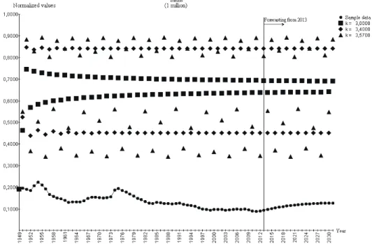
Let’s have a closer look at the two most important demographic indicators:
population and birth, the main economic indicator: GDP and the leading cause of deaths due to cardiovascular diseases in the diagrams. The figures show where the curves of the actual data are running in the analysed period compared to the set of curves (bifurcation lines) generated mathematically using three significant values of k – 3, 3.4, and 3.57 –, and they also show the forecasting from 2013 (from 2014 for the GDP).
41
Figure 1. Population with forecasting from 2013
We can see in figure 1, that the population time series of the country (circles) are running far below all the bifurcation lines (square, diamond and triangle), thus below the alternatives that may bring qualitative change. According to the results of our method, we cannot expect any significant change, the course of the indicator is stable and it is likely to keep following that in the future.
42
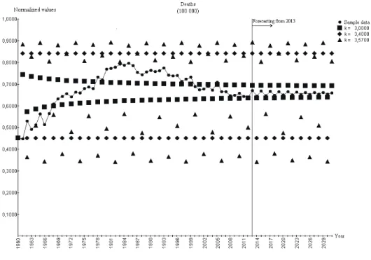
Figure 2. Live births with forecasting from 2013
It can be read from figure 2, that the actual data – like the population – is running way below the bifurcation lines, which we can conclude from, that the opportunity of change is far away. In spite of a few peaks protruding from the curve of the time series, even they don’t approach the bifurcation lines.
43
Figure 3. GDP index with forecasting from 2014
The course of the GDP is much more changeable than the previous two indicators, it draws close to the lower bifurcation lines in the late 1980’s and in the early 1990’s, and it ascends in between the lower bifurcation lines in the 2000’s. It makes us come to the conclusion that the economy was at a crossroads, however the curve does not ascend between the upper bifurcation lines indicating that the realized alternative course was not the best one. The curve descending below the bifurcation lines tells us that it is moving away from the chance of change.
44
Figure 4. Number of deaths due to cardiovascular diseases with forecasting from 2013 The number of deaths due to cardiovascular diseases is the most dynamically changeable time series. Its course is going between the bifurcation lines all along, thus the opportunity of change is present all the time. If a selected characteristic of a subsystem has such a behavior, then we may assume that significant change can be achieved by a small effort. In this particular case, what the leading cause of death is in Hungary nowadays, could be forced to a lower level by enacting a relatively focused effort.
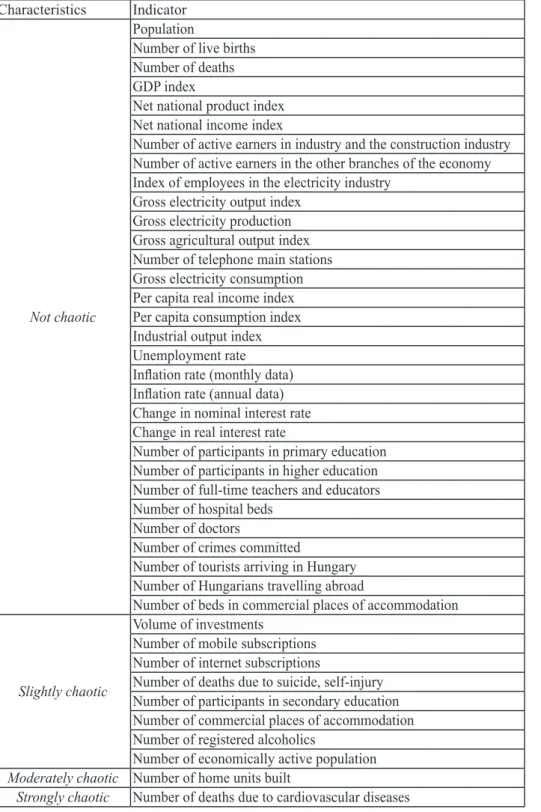
As we can see after analysing the indicators, the characteristic of the Hungarian macro indicators is not chaotic: the behaviour of 31 indicators out of the 41 is not chaotic. Amongst the 10 indicators tending to be chaotic, 8 belong to the slightly chaotic (volume of investments, number of mobile subscriptions, number of internet subscriptions, number of deaths due to suicide, self-injury, number of participants in secondary education, number of commercial places of accommodation, number of registered alcoholics, number of economically active population). One indicator (the number of home units built) displays moderately chaotic behaviour, while the number of deaths due to cardiovascular diseases has strongly chaotic behaviour.
45
Table 2. Overall view of the behavior of the chosen indicators Characteristics Indicator
Not chaotic
Population
Number of live births Number of deaths GDP index
Net national product index Net national income index
Number of active earners in industry and the construction industry Number of active earners in the other branches of the economy Index of employees in the electricity industry
Gross electricity output index Gross electricity production Gross agricultural output index Number of telephone main stations Gross electricity consumption Per capita real income index Per capita consumption index Industrial output index Unemployment rate Inflation rate (monthly data) Inflation rate (annual data) Change in nominal interest rate Change in real interest rate
Number of participants in primary education Number of participants in higher education Number of full-time teachers and educators Number of hospital beds
Number of doctors
Number of crimes committed
Number of tourists arriving in Hungary Number of Hungarians travelling abroad
Number of beds in commercial places of accommodation
Slightly chaotic
Volume of investments
Number of mobile subscriptions Number of internet subscriptions
Number of deaths due to suicide, self-injury Number of participants in secondary education Number of commercial places of accommodation Number of registered alcoholics
Number of economically active population Moderately chaotic Number of home units built
Strongly chaotic Number of deaths due to cardiovascular diseases
Own compilation
46
Consequently the most important proceedings in the society and economy are following stable courses in general, they have not been in chaotic state in the past and the onset of chaos cannot be expected in the future either. Only a few of the indicators display some tendency to behave chaotically. The indicator of the home units built is the easiest to turn to more desirable courses, and some of the indicators related to health and social states also seems to be easier to change. The area of modernization seems to be similar, and it may even come to improve itself. There are some minor possibilities in the employment, investments, secondary education and tourism. The number of deaths due to cardiovascular diseases is worth noticing, since its behaviour is strongly chaotic, that is, it is relatively easy to modify its course to both better or worse directions.
Those areas where the chance exists to improve demands high attention, because missing these chances may lead toward letting those indicators run on undesirable courses, and some of the worse alternatives may be realized left on their own. It is also important to turn those processes to desirable courses, because they interact.
They affect those processes that run on stabilized courses at the moment. It means that making some changes where it is easier may be the initial step towards making changes to processes stabilized for now and which are more difficult to improve at the moment.
Comparing the results from twenty years back
We compare the results of the present analysis and the results of the analysis done twenty years ago (see Nováky, Hideg, and Gáspár-Vér, 1997) to let us see if the behaviour of the analysed indicators has become less chaotic, thus the processes of our economy and our society has become more stable, leading to decreasing chances for change, or whether they became more chaotic, thus suggesting the availability of better chances to improve situations through targeted interventions. The analysis done in 2014 allows us to see which courses of bifurcations – forecasted 20 years ago – were realized, or towards which of them the indicators started to approach.
Demographic indicators
The population has not changed a bit in the past several decades. It remained as stable as before, it still runs far below the bifurcation lines just like the forecasting showed. It supports the idea, that it is extremely difficult to turn the behaviour of this characteristic of our society to a better course. The number of live births behaves less chaotically than it did twenty years ago, now it is completely chaos free, contrary to its slightly chaotic behaviour earlier. It is still characterized by a slow decline. The change in the number of deaths is nearly nothing, the value of its coefficient virtually settled right where it was twenty years ago, the indicator stabilized at a level a bit lower than it was twenty years ago after a subtle descent.
Socio-economic indicators
The GDP has had a not chaotic behaviour for the last 40 years, in spite of being moderately chaotic in the period 20 years ago. The net national product and net national income have also stabilized and the slightly chaotic behaviour was replaced by the purely not chaotic behaviour.
The value of the coefficient of the number of economically active population
47
decreased a bit, the result of the earlier calculation of that was 2.05, so it was moderately chaotic, now it is 1.96, right below that range. In accordance with the calculation twenty years ago, the indicator seems to stabilize.
The volume of investments turned out to be more stable as well, the value of the coefficient from 1.78 – that suggests a slightly chaotic behaviour – decreased to 1.5, the lower limit of the same range. The curve of the indicator ascended to the upper part of the lower range of the bifurcation lines and started to descend recently and according to the forecasting it does run between the lower bifurcation lines.
The number of home units built decreased from the chaotic value of 2.6 to 2.16 which is still chaotic, but it is very close to the lower limit of that range. In spite of the forecasting it does not run at the top of the lower bifurcation lines, instead it fluctuates around the lower range of them, or under them many times.
The number of participants in primary education (k decreased from 1.15 to 1.12) runs under the lower bifurcation lines, like the forecasting suggested. The number of participants in secondary education became significantly chaotic, the value of k increased from 1.06 to 1.69, thus from being not chaotic it became slightly chaotic. The forecasting suggested otherwise, as the indicator does not run below the bifurcation lines, but ascends to the upper part of the lower bifurcation lines and settles there. The coefficient of the number of participants in higher education increases from 1.13 to 1.25, the indicator got between the lower bifurcation lines after a steep ascension, then it started to descend, and it is not running parallel with the bifurcation lines. The number of full-time teachers and educators stabilized. Its coefficient was 1.979 (so almost moderately chaotic), but it dropped to 1.2, which means it became not chaotic. The curve runs far below the bifurcation lines so it is different from the forecasting course that put the indicator into the upper third of the lower range of bifurcation lines.
The value of k characterizing the deaths due to cardiovascular diseases increases from the moderately chaotic 2.789 (being very close to the upper limit) to the strongly chaotic 2.92. The behaviour is in accordance with the results of the forecasting, its variation diminishes, the curve is between the lower and upper range of bifurcation lines. The number of registered alcoholics turns from moderately chaotic (2.343) to slightly chaotic (1.88), dropping significantly, but it is not realistic as it was explained earlier. The number of deaths due to suicide, self-injury moved a little toward stabilization, but remained slightly chaotic, the coefficient is still decreasing slowly. Its stabilization can’t be taken for granted, so the only part of the forecasting that became real is that it decreased but it did not stabilize.
The k characterizing the number of commercial places of accommodation increased in the slightly chaotic range. This is completely different from the forecasting, it ascends steeply above the bifurcation lines to the top of the whole range. The coefficient of the beds in commercial places of accommodation dropped from 3.769 to 1.1, the purely chaotic characteristic was replaced by a not chaotic behaviour. It is completely different from the forecasting, since it runs far below the bifurcation lines, approaching them only a very little.
Summarizing what has happened in the last 20 years, most of the indicators became less chaotic, which means that the socio-economic processes stabilized generally in the past two decades. Out of the compared 38 indicators (we included two more indicators into our research in 2014, but there was nothing to compare them to, and the previous research analysed the inflation rate with monthly time
48
series only), the k value characterizing the data of the time series stabilized in 25 cases. Out of those 25 indicators, the change is not significant in 12 cases (“descent is not significant”), and there is significant stabilizing in the remaining 13 cases. The number of beds in commercial places of accommodation decreased by three levels (“from strongly chaotic it became not chaotic”), the index of the GDP decreased by two levels (“from moderately chaotic it became not chaotic”). Two indicators – the number of home units built and the number of registered alcoholics – have changed by one level only (“from moderately chaotic they became slightly chaotic”), but the behaviour of these indicators is still chaotic (though slightly chaotic only). The rest (9) of the indicators – the net national product index, the net national income index, the gross electricity production, the volume of investments, the gross electricity consumption, the number of full-time teachers and educators, the number of hospital beds, the number of doctors and the number of crimes committed – have also changed by one level only, but their behaviour left the range of chaos entering the not chaotic range. We don’t expect these indicators to change significantly.
In the past 20 years the k value of one indicator (the inflation rate) remained unchanged, that of 12 indicators has increased, out of them the value of nine has not changed significantly (they remained at the same level of not chaotic). The indicators of the number of participants in secondary education and the number of commercial places of accommodation changed their behaviour in quality: they increased by one level (“from not chaotic they became slightly chaotic”). We have our positive expectations towards these indicators and those that have been behaving chaotically for a longer time. The number of deaths due to cardiovascular diseases has also increased by one level, thus it left the moderately chaotic range entering the strongly chaotic range, which we don’t consider favourable at all. Thus the changes in the future cannot be expected either from the indicators related to material production or investments, or staff in education, or the equipment for hospitals and accommodations. The group of indicators that may advance development is in the state of reshaping and renewing.
Conclusions
We can come to the conclusion from the behaviour of the macro indicators, and this is our final conclusion – similar to the one in 1995 – that the Hungarian society and economy is not in the state of chaos, the indicators became more and more stable, they settle. The chance to change them is slowly getting lost, it will be more and more difficult to renew the Hungarian socio-economic indicators, and to turn the processes to more desirable courses.
The changes in the future can be expected from the service sector of the economy, the number of home units built, the number of participants in secondary education, the number of deaths due to cardiovascular diseases and the number of commercial places of accommodation. Thus the key to the future lies in the secondary education and the health of the population.
It must be clear by now, that the Hungarian society and economy does not only have one way to go, but several alternative courses are given to follow. A better situation may be expected to come as well as ending up in some undesirable conditions. The renewing, creative power of chaos is required for the Hungarian society and economy to rearrange in quality, rise to a higher level and advance toward a more harmonic civilian society.
49
Significant positive changes to ensue in Hungary needs more attention placed on human factors, – by providing the conditions for improvements in education, healthy life styles and favourable accommodation and housing.
Correspondence
Prof. Dr. Erzsébet Nováky Corvinus University of Budapest
Email: erzsebet.novaky@uni-corvinus.hu Miklós Orosz
Tata Consultancy Services Email: miklos.orosz@t-online.hu
Notes
1 See Nováky, Erzsébet (ed.) (1995). Káosz és jövőkutatás. [Chaos and futures studies] Budapest: Budapesti Közgazdaságtudományi Egyetem Jövőkutatás Tanszék.
Nováky, Erzsébet, Hideg, Éva, and Gáspár-Vér, Katalin. (1997). Chaotic Behaviour of Economic and Social Macro indicators in Hungary. Journal of Futures Studies, 1(2), 11-31.
2 Orosz, Miklós. (2014). Társadalmi-gazdasági mutatók vizsgálata káoszelméleten alapuló eszközökkel. [Analysing socio-economic indicators by the methods based on chaos theory] Jövőtanulmányok 27. Budapest: Corvinus University of Budapest.
59 p.
3 The choice of time series was guided by the book Káosz és jövőkutatás (edited by Erzsébet Nováky) [Chaos and Futures Studies], chapter Hazai makromutatók kaotikus viselkedéséről [About the chaotic behaviour of Hungarian macro indicators]. We mainly followed it choosing the analysed indicators.
References
Chiarella, C. (1988). Experimental Mathematics: The Role of Computation in Non- linear Science. Economic modelling, 28(4), 376-384. Retrieved on March 11, 2013, from http://fisica.ufpr.br/viana/economia/chiarella.pdf
Campbell, D., Crutchfield, J. P., Farmer, J. D., and Jen, E. (1985). Experimental Mathematics: The Role of Computation in Nonlinear Science. Communica- tions of the Association for Computing Machinery, 28(4), 374-384.
Fokasz, Nikosz. (2000). Káosz és fraktálok, Bevezetés a kaotikus dinamikus rendsze- rek matematikájába szociológusok számára. [Chaos and fractals. Introduction to the mathematics of chaotic dynamical systems for sociologists] Budapest:
Új Mandátum Könyvkiadó.
Fokasz, Nikosz. (ed.) (2002). A káoszkutatás új eredményei. [The latest results of chaos research] Magyar Tudomány, 47(10), 1272-1273.
Fokasz, Nikosz. (2002). Nemlineáris idősorok – A tőzsde káosza? [Nonlinear time series – The chaos of stock market?] Magyar Tudomány, 47(10),1312-1329.
Gáspárné Vér, Katalin, Hideg Éva, and Nováky, Erzsébet. (1995). A társadalmi-gaz- dasági makromutatók és a káoszelmélet. [The socio-economic macro indica-
50
tors and the chaos theory] Statisztikai Szemle, 73(12), 976-989.
Gleick, James. (1987). Chaos: making a new science. New York: Viking Penguin.
Gruiz, Márton, Tél, Tamás. (2005). A káosz. Egy szokatlan és mégis gyakori moz- gásforma. [The chaos. An unusual still frequent form of movement] Fizikai Szemle, 55(5), 191-193.
Heino, A. (2004). The Future Workshop. Deutsches Institut für Erwachsenenbildung, März. Retrieved on October 12, 2004, from http://www.die-bonn.de/esprid/
dokumente/doc-2004/apel04_02.pdf
Nováky, Erzsébet. (1993). Jövőkutatás és káosz. [Futures studies and chaos]. Ma- gyar Tudomány, 38(4), 512-517.
Nováky, Erzsébet. (ed.) (1995). Káosz és jövőkutatás. [Chaos and futures studies]
Budapest: Budapesti Közgazdaságtudományi Egyetem Jövőkutatás Tanszék.
Nováky, Erzsébet. (1995). Káosz és előrejelzés. [Chaos and forecasting] Statisztikai Szemle, 73(10), 815-823.
Nováky, Erzsébet. (2003). A jövőkutatás módszertana stabilitás és instabilitás mel- lett. [Methodology of futures studies with stability and instability] Budapest:
Budapesti Közgazdaságtudományi és Államigazgatási Egyetem Jövőkutatási Kutatóközpont.
Nováky, Erzsébet, Hideg, Éva, and Gáspár-Vér, Katalin. (1997). Chaotic Behaviour of Economic and Social Macro Indicators in Hungary. Journal of Futures Studies, 1(2), 11-31.
Nováky, Erzsébet, Orosz, Miklós. (2015). A hazai társadalmi-gazdasági mutatók vizsgálata a káoszelmélet eszközével. [Analysing Socio-Economic Indicators by the Method of Chaos Theory]. Statisztikai Szemle, 93(1), 25-52.
Orosz, Miklós. (2014). Társadalmi-gazdasági mutatók vizsgálata káoszelméleten alapuló eszközökkel. [Analysing socio-economic indicators by the methods based on chaos theory] Jövőtanulmányok 27. Budapest: Corvinus University of Budapest. 59 p.
Szépfalusy, Péter (ed.), Tél Tamás (ed.) (1982). A káosz. Véletlenszerű jelenségek nemlineáris rendszerekben. [The chaos. Random phenomena in nonlinear systems] Budapest: Akadémiai Kiadó.
Tél, Tamás, Gruiz, Márton. (2002). Mi a káosz? (És mi nem az). [What is chaos?
(And what it is not)] Természet Világa, 133(7), 296-298.
Wikipedia, Future workshop. Retrieved on November 23, 2013, from http://
en.wikipedia.org/wiki/Future_workshop
Wikipedia, Dynamical billiards. Retrieved on November 23, 2013, from http://
en.wikipedia.org/wiki/Dynamical_billiards
Wikipedia, Baker’s map. Retrieved on November 23, 2013, from http://
en.wikipedia.org/wiki/Baker’s_map
Wikipedia, Arnold’scat map. Retrieved on November 23, 2013, from http://
en.wikipedia.org/wiki/Arnold’s_cat_map
Wikipedia, Hénon map. Retrieved on November 23, 2013, from http://en.wikipedia.
org/wiki/Hénon_map