State subsidy and moral hazard in corporate financing
by Edina Berlinger, Anita Lovas, Péter Juhász
C O R VI N U S E C O N O M IC S W O R K IN G P A PE R
http://unipub.lib.uni-corvinus.hu/2185
CEWP 22/ 201 5
1 Edina Berlinger, Department of Finance, Corvinus University of Budapest1
Anita Lovas, Department of Finance, Corvinus University of Budapest2 Péter Juhász, Department of Finance, Corvinus University of Budapest3
December 27th 2015
Acknowledgement: This paper was based on work supported by the Hungarian Academy of Sciences, Momentum Programme (LP-004/2010) and by the research grant of Corvinus University of Budapest, Corvinus Business School.
Abstract
This paper investigates the impact of state subsidy on the behavior of the entrepreneur under asymmetric information. Several authors formulated concerns about state intervention as it can aggravate moral hazard in corporate financing. In the seminal paper of Holmström and Tirole (1997) a two-player moral hazard model is presented with an entrepreneur initiating a risky scalable project and a private investor (e.g. bank or venture capitalist) providing outside financing. The novelty of our research is that this basic moral hazard model is extended to the case of positive externalities and to three players by introducing the state subsidizing the project. It is shown that in the optimum, state subsidy does not harm, but improves the incentives of the entrepreneur to make efforts for the success of the project; hence in effect state intervention reduces moral hazard. Consequently, state subsidy increases social welfare which is defined as the sum of private and public net benefits. Also, the exact form of the state subsidy (ex-ante/ex-post, conditional/unconditional, refundable/nonrefundable) is irrelevant in respect of the optimal size and the total welfare effect of the project. Moreover, in case of nonrefundable subsidies state does not crowd out private investors; but on the contrary, by providing additional capital it boosts private financing. In case of refundable subsidies some crowding effects may occur depending on the subsidy form and the parameters.
Keywords: contract theory, externalities, asymmetric information, crowding out JEL code: D28, D86, G38, H23, H81
1 edina.berlinger@uni-corvinus.hu, phone: +36305541075, fax: +3614825212
2 anita.lovas@uni-corvinus.hu
3 peter.juhasz@uni-corvinus.hu
2 1. Introduction
In the literature, there have been made serious efforts to understand the effects of state subsidy in corporate financing in case of asymmetric information which may have two negative consequences: adverse selection and moral hazard. As it is summarized in Kotowitz (2008, page 6), the results are mixed: „The existence of such inefficiencies signals a possible role for government. However, government intervention may well cause more problems than it solves… It is therefore unclear whether government supply of these services enhances welfare.”
Takalo and Tanayama (2010), and Kleer (2010) focused on the adverse selection problems in the framework of theoretical models, and concluded that state subsidy may help to resolve this kind of market failure. On the other hand, Chaney and Thakor (1985) examined the moral hazard and demonstrated that loan guarantees provided by the state create perverse incentives for the firms. Keuschnigg and Nielsen (2001) concluded that in the venture capital industry direct subsidies distort incentives, hence do not improve social welfare at all; while soft tools like improving training, information and infrastructure may be effective. Schertler (2000, 2002a, 2002b), and Hirsch (2006) also investigated the role of state subsidy in the financing of innovative, early stage enterprises with double-sided moral hazard, where both entrepreneurs and private investors (venture capitalists) had to make efforts to contribute to the success of the project. According to their results, state subsidy compromises the incentives, hence aggravates moral hazard.
There is also a large empirical literature dealing with the effectiveness of state subsidy systems. Different countries’ data have been analyzed, see Table 7 in Annex 2. Although data and methods are different, there is more or less consensus that state subsidy creates value at social level which is mostly due to the positive externalities of the projects and to the role of state subsidy in lifting capital constraints. Meanwhile, the low efficiency of certain projects is supposed to be caused by adverse selection and moral hazard, especially in case of large firms. Also, different authors disagree on the optimal form and on the crowding out effect of the state subsidy.
Contrary to this, in our three-player moral hazard model where the project has positive externalities, it is shown that in the optimum, state subsidy effectively reduces moral hazard, hence its overall effect is always positive; moreover, the form of subsidy is irrelevant. We define six different state subsidy forms within a simple one-period and two-outcome project, and we conclude that although the inner structures of the optimal contracts are different, the optimal size of the state subsidy and the induced total social welfare are the same for each subsidy form. Moreover, we also show that pure grants have no crowding out effect, while in case of subsidized loans the crowding out effect depends on the subsidy form and the parameters.
Our model is a generalization of the previous moral hazard investigations in corporate financing which focused on private parties contracting without state intervention. This topic
3 has been emerging from the seminal papers of Shavell (1979), Sappington (1983), Grossman and Hart (1983), Laffont and Tirole (1988), Holmström and Tirole (1997), Hart and Moore (1998), and Tirole (2006). The basic model we build on is Holmström and Tirole (1997) as the explicit formalization of the variable size investment problem was first presented there.
In Section 2 we summarize the basic moral hazard model with two players (entrepreneur and investor) in order to give a better foundation for our model discussed in Section 3 where we introduce state as a new player representing the social interests. First, we set out potential state subsidy forms; then present our three-player model (entrepreneur, investor and state) and derive the optimum for each subsidy form. In Section 4 we evaluate our findings by comparing the results of different settings, and finally we derive conclusions in Section 5.
2. The two-player model
As in Holmström and Tirole (1997) the entrepreneur owns a scalable project with constant rate of return. The initial investment is 𝐼 > 0, and the entrepreneur has an initial asset 𝐼 > 𝐴 > 0. The missing financing, 𝐼– 𝐴 should be acquired from an outside private investor.
On the top of this basic model we introduce the positive externalities of the project as a new element.
Assumption 1 (Unconditional positive externalities) The project has positive externalities which are independent of the success of the project (for example increased employment, economic activity of the suppliers, knowledge transfer), can be expressed in nominal value, and are proportional to the investment’s size (𝐸𝐼, where 𝐸 > 0). We assume that these externalities are directly realized by the state in the form of explicit incomes or savings in the state budget at the end of the project. Of course, private contracting parties (entrepreneur, investor) do not take these external effects into consideration on their own.
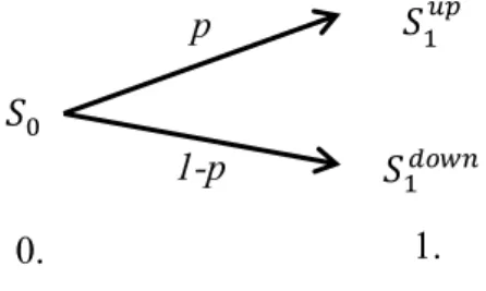
The project is one period long (between t=0 and t=1) and has two outcomes: success with probability 𝑝 or failure with probability 1 − 𝑝. Besides the externalities, in case of success the project pays a return proportional to the investment’s size (𝑅𝐼, where 𝑅 > 1), while in failure the project pays no return, as it can be seen on Figure 1.
Figure 1: Project cash-flows
Source: Tirole (2006) with modification I
RI+EI
EI p
1-p
0. 1.
4 The probability of the success (p) depends on the entrepreneur’s behavior which is not directly observable by the investor. In case of high efforts (behaving) the probability is 𝑝 = 𝑝𝐻, while in case of low efforts (misbehaving) 𝑝 = 𝑝𝐿 where 𝑝𝐻 > 𝑝𝐿. Moreover, the entrepreneur realizes private benefit (𝐵𝐼 > 0) by misbehaving for example in forms of increased utility of shirking, perks and other hidden personal gains which are unavailable for the investor.
Hence, we face a typical principal-agent problem where the principal is the investor and the agent is the entrepreneur; and the investor has naturally less information on the efforts of entrepreneur than the entrepreneur himself which raises the issue of moral hazard.
For the sake of simplicity and without loss of generality time preferences are excluded and investors are supposed to be perfectly competitive.
Assumption 2 (Risk neutrality) Both players are risk neutral, hence they are interested only in expected values.
It follows from our assumptions that the expected return of the investors is supposed to be zero.
Assumption 3 (Relevance of moral hazard) The net present value (NPV) of the project (without the externalities) is positive only in the case of high efforts:
𝑁𝑃𝑉𝑏𝑒ℎ𝑎𝑣𝑒 > 0 > 𝑁𝑃𝑉𝑚𝑖𝑠𝑏𝑒ℎ𝑎𝑣𝑒 𝑝𝐻𝑅𝐼 − 𝐼 > 0 > 𝑝𝐿𝑅𝐼 − 𝐼 + 𝐵𝐼
𝑝𝐻𝑅 > 1 > 𝑝𝐿𝑅 + 𝐵 (1)
Due to requirement (1) moral hazard does matter, as financing is possible only if the entrepreneur behaves. If both 𝑁𝑃𝑉𝑏𝑒ℎ𝑎𝑣𝑒 and 𝑁𝑃𝑉𝑚𝑖𝑠𝑏𝑒ℎ𝑎𝑣𝑒 were positive, there would be no financing constraint at all, and the optimal size of the project would be infinite. On the other hand if both NPVs were negative there would be no point in investing and financing for the private parties at all.
As it can be seen on Figure 1, the success of the project depends also on the environment (chance), as the project is possible to succeed in case of low efforts, as well. It should be also noticed that the investor is considered to be passive given that the probability of success is independent of his behavior once the financing is provided.4
4 In case of venture capital investments the investor is actively working on the project, hence we face a double moral hazard problem, see (Schertler 2000, 2002a, 2002b) and (Hirsch 2006).
5 Assumption 4 (Liability) The entrepreneur has limited liability, while the investor has unlimited liability. Hence, the entrepreneur‘s future return must be nonnegative in any cases, but the investor’s future return can be of any sign. 5
Contract design has to answer two questions:
- What is the optimal size of the project (𝐼)?
- How much the entrepreneur and the investor gets in case of success, (𝑅𝑒) and (𝑅𝑖); and in case of failure, (𝑟𝑒) and (𝑟𝑖)?
We note that there are only two outcomes of the project, therefore we cannot differentiate between convex (equity) and concave (debt) repayment forms. Hence, the outside investor can be considered as a shareholder or as a lender, it is not specified in the model.
The entrepreneur maximizes his welfare by offering a contract to the investor who can accept or refuse it. In a classical principal-agent model it is usually the principal who offers the contract to the agent. However, in Holmström and Tirole (1997) it is the agent (the entrepreneur) who takes the initiative. This may seem strange for the first sight. The reason behind this setting is that investors are operating on a perfectly competitive market and it is the entrepreneur who has a particular project of positive NPV; hence the value is created on his side. This is why he has the bargaining power to offer the contract. The timing of the project is presented on Figure 2.
Figure 2: The timing of the two-player project
Source: Tirole (2006)
When designing the contract, the entrepreneur maximizes his welfare (his net expected benefit):
max 𝑝𝐻𝑅𝐼 − 𝑝𝐻𝑅𝑖 − (1 − 𝑝𝐻)𝑟𝑖− 𝐴 (2) with respect to some constraints. First of all, the contract must ensure that the entrepreneur has interest to behave, otherwise NPV would be negative, and the investor would refuse to finance it. This requirement can be expressed as
𝑝𝐻𝑅𝑒+ (1 − 𝑝𝐻)𝑟𝑒 ≥ 𝑝𝐿𝑅𝑒+ (1 − 𝑝𝐿)𝑟𝑒+ 𝐵𝐼
5 Investors are supposed to hold a large diversified portfolio and this project is just one element of it. Hence, with regard to this special project they can be supposed to have unlimited liability.
investor accepts or not
entrepreneur behaves or
not
project succeeds
or not
sharing of the return entrepreneur
offers a contract
6 meaning that behaving should be more attractive than misbehaving for the entrepreneur.
Applying the notation of 𝑝𝐻− 𝑝𝐿 = ∆𝑝, the incentive constraint of the entrepreneur (ICe) can be simplified to
ICe 𝑅𝑒− 𝑟𝑒≥ 𝐵𝐼
∆𝑝
(3)
Secondly, also the investor should have interest to participate (PC - participation constraint) by getting back at least his investment (F):
PCi 𝑝𝐻𝑅𝑖 + (1 − 𝑝𝐻)𝑟𝑖 ≥ 𝐹 (4)
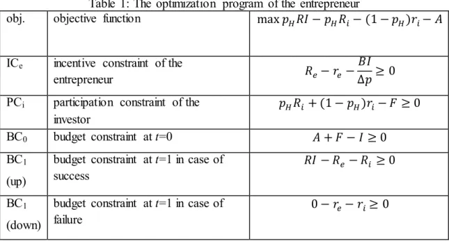
Other constraints come from the budget constraints (BC) at 𝑡 = 0 and 𝑡 = 1 as it is not possible to spend more what is disposable. The optimization problem of the entrepreneur is summarized in Table 1.
Table 1: The optimization program of the entrepreneur
obj. objective function max 𝑝𝐻𝑅𝐼 − 𝑝𝐻𝑅𝑖− (1 − 𝑝𝐻)𝑟𝑖− 𝐴
ICe incentive constraint of the
entrepreneur 𝑅𝑒− 𝑟𝑒 −𝐵𝐼
∆𝑝≥ 0 PCi participation constraint of the
investor
𝑝𝐻𝑅𝑖 + (1 − 𝑝𝐻)𝑟𝑖− 𝐹 ≥ 0
BC0 budget constraint at t=0 𝐴 + 𝐹 − 𝐼 ≥ 0
BC1
(up)
budget constraint at t=1 in case of success
𝑅𝐼 − 𝑅𝑒− 𝑅𝑖 ≥ 0
BC1
(down)
budget constraint at t=1 in case of failure
0 − 𝑟𝑒− 𝑟𝑖≥ 0
Source: authors, based on Holmström and Tirole (1997)
Parameters like 𝑅, 𝐴, 𝑝𝐻, 𝑝𝐿,𝐵 are given exogenously and there is no uncertainty about their values. While parameters like 𝐹, 𝐼, 𝑅𝑒, 𝑅𝑖, 𝑟𝑒, 𝑟𝑖 are decision variables to be determined in the contract as a result of the optimization program in Table 1.
Assumption 5 (No reward in failure) In case of failure the entrepreneur receives no reward.
It is a natural idea that the entrepreneur is not rewarded in case of failure as he is the only one responsible for the success of the project.
Combining Assumption 4 and Assumption 5, we get that in case of failure, the return of the entrepreneur, 𝑟𝑒, cannot be either negative (limited liability of the entrepreneur) or positive (no reward in failure), thus it should be zero (𝑟𝑒 = 0).
7 Proposition 1 (Optimum without state subsidy) There exists only one solution to the problem in Table 1. In this optimum
- the size of the investment is
𝐼 = 1
1 − 𝑝𝐻(𝑅 − 𝐵∆𝑝)
𝐴 = 1
1 − 𝜌0A (5)
where 𝜌0 is the so called pledgeable income (the maximum amount the entrepreneur can promise to the investor without the risk of moral hazard in case of a one-dollar investment), see Tirole (2006).
It follows from Assumption 3 that the pledgeable income is always positive. Given that the size of the investment (𝐼) and the initial liquid asset (𝐴) are supposed to be positive, we also know that in the optimum the pledgeable income is less than one:
0 < 𝜌0 < 1.
- the private financing is
𝐹 = 𝜌0
1 − 𝜌0𝐴 (6)
- the share of the investor in case of success is 𝑅𝑖 = 𝜌0
𝑝𝐻(1 − 𝜌0)𝐴 (7)
- the share of the investor in case of failure is
𝑟𝑖 = 0 (8)
- the share of the entrepreneur is in case of success is
𝑅𝑒 = 𝑝𝐻𝑅 − 𝜌0
𝑝𝐻(1 − 𝜌0)𝐴 (9)
Proof The multivariate optimization problem can be solved by applying the Kuhn-Tucker method. The corresponding Lagrange function is
ℒ = 𝑝𝐻𝑅𝐼 − 𝑝𝐻𝑅𝑖 − (1 − 𝑝𝐻)𝑟𝑖− 𝐴 − 𝜆1(𝐵𝐼
∆𝑝− 𝑅𝑒− 𝑟𝑒) − 𝜆2(𝐹 − 𝑝𝐻𝑅𝑖− (1 − 𝑝𝐻)𝑟𝑖)
− 𝜆3(𝐼 − 𝐴 − 𝐹) − 𝜆4(𝑅𝑒+ 𝑅𝑖− 𝑅𝐼) − 𝜆5(𝑟𝑒+ 𝑟𝑖)
Considering the necessary and sufficient conditions of the optimum, it can be easily seen that all lambdas are positive; hence all the five constraints are fulfilled with equality. Applying
8 Assumption 5 (𝑟𝑒 = 0) we have five variables (𝐼,𝐹, 𝑅𝑒, 𝑅𝑖, 𝑟𝑖) and five independent equations, hence the solution is unique and Equations (6-9) can be derived by simple algebra. □
The main conclusions of the two-player model can be summarized as follows:
- We can see from Equation (5) that the size of the investment (𝐼) is limited by the initial asset of the entrepreneur (𝐴). The entrepreneur would be interested to increase the project size to infinity (his net benefit would go to infinity too); but at a certain level of initial asset, moral hazard puts restraint to the outside financing, hence to the project size, as well. Accordingly, the model provides an equilibrium explanation of credit rationing (i.e. why financial markets do not always clear by price adjustment), Tirole (2006).
- Loan is accredited only if good behavior of the entrepreneur is assured. Hence the problem of moral hazard is fully solved by the incentives set up in the contract at the beginning of the project. No further tools, like costly monitoring, are needed.
- The entrepreneur receives the entire surplus of the project (𝑁𝑃𝑉 = 𝑝𝐻𝑅𝐼 − 𝐼); this keeps him motivated to behave.
- The project has positive external effects on the state budget (𝐸𝐼); but as the size of the investment is constrained, external effects are also constrained by the agency problem.
- The initial asset of the entrepreneur has shadow value in the sense that one additional dollar invested in the project would create additional NPV (and positive externalities).
It follows from this that the entrepreneur has interest to invest all his capital into the project.
It is also shown that even if we remove Assumption 5 (No reward in failure), any reward to the entrepreneur in failure would be suboptimal (Tirole 2006, page 116.). By all means, it is obviously not a good idea to compensate the entrepreneur for the failure as it would destroy his incentives to behave.
In the next part we examine what happens if state intervenes in favor of social welfare.
3. The three-player model
In order to analyze the impact of state subsidy on the project financing under moral hazard we introduce state as the third player while keeping most of the model’s assumptions unchanged.6 We assume that in the first round the state offers a contract to the entrepreneur. This contract defines the size (𝑆 > 0) and other conditions of the subsidy. The entrepreneur may decide to take it or leave it. If the subsidy contract is accepted by the entrepreneur, then, in the second round, based on the available state subsidy the entrepreneur offers a contract to the private investor exactly as in Holmström and Tirole (1997) where the invested private capital
6 Csóka et al. (2015) also developed the same basic model by introducing a new player: the buyer of the entrepreneur.
9 provided by investor (𝐹), the size of the project (𝐼), the return to the entrepreneur in success and in failure (𝑅𝑒, 𝑟𝑒), and the return to the investor in success and in failure (𝑅𝑖, 𝑟𝑖) are settled down. The timing of the three-player project is illustrated on Figure 3.
Figure 3: Timing of the three-player model
Source: the authors
As one can see on Figure 3, the new elements compared to Figure 2 are only due to the presence of the state which intervenes at the beginning of the project, all the rest remains the same as in Holmström and Tirole (1997).
We note that in principle it is also possible that state gives the subsidy to the private investor in order to encourage private lending. It can be shown that this would not influence the outcome of the model, mainly because when formulating the subsidy contract state considers the interests of all players.7
3.1 Forms of state subsidy
In the framework of the above described, simple, one-period and two-outcome project, logically there exist six different forms of state subsidies. If a state subsidy is non-refundable, theoretically it can be received either at the beginning or at the end of the project. In the latter case it can be awarded either in success or in failure.8 We get three possibilities:
1. nonrefundable ex-ante subsidy
2. nonrefundable ex-post subsidy received in case of success
3. nonrefundable ex-post subsidy received in case of failure (e.g. guarantee)
If a state subsidy is refundable, it can be required to be refunded in any case (unconditional) or only in case of success or in case of failure (conditional):
4. refundable ex-ante subsidy
5. refundable ex-ante subsidy repaid in case of failure 6. refundable ex-ante subsidy repaid in case of success
All these six subsidy forms exist in the real world international practice, and logically they cover all the possibilities corresponding to a project of the general scheme of Figure 4.
7 Berlinger et al. (2015) present a model where the players (state, entrepreneur and private investor) make a three-sided contract in one round.
8 If it is given out at the end irrespectively whether the project succeeds or fails, it can be considered as the combination of the two (forms 2 and 3).
investor accepts or not
entrepreneur behaves or
not
project succeeds
or not
sharing of the return entrepreneur
offers a contract to private investor state offers
a contract to entrepreneur
entrepreneur accepts
or not
10 Figure 4: The structure of the state subsidy
Source: the authors
Definition 1 (Net present value of state subsidy) In each form of state subsidies the net present value of the subsidy (𝑆̅) is calculated as the sum of the expected value of all cash- flows at t=0:
𝑆̅ = 𝑆0+ 𝑝𝑆1𝑢𝑝+ (1 − 𝑝)𝑆1𝑑𝑜𝑤𝑛 (10) Table 2 summarizes state subsidies of different dimensions. Cash-flows are presented from the entrepreneur’s perspective (𝑆 is an inflow for the entrepreneur but an outflow for the state).
Table 2: State subsidy forms and their cash-flows from the entrepreneur's perspective
Unconditional Conditional
Reward in success Rescue in failure
Non refundable
1. Nonrefundable ex-ante subsidy
𝑆̅ = 𝑆
2. Ex-post subsidy in case of success
𝑆̅ = 𝑝𝑆
3. Ex-post subsidy in case of failure
𝑆̅ = (1 − 𝑝)𝑆
Refundable
4. Refundable ex-ante subsidy
𝑆̅ = 0
5. Ex-ante subsidy refundable in failure
𝑆̅ = 𝑝𝑆
6. Ex-ante subsidy refundable in success
𝑆̅ = (1 − 𝑝)𝑆 Source: the authors
Four subsidies are received ex-ante (1, 4, 5, 6), and two of the subsidies are received ex-post (2, 3). Two of them are unconditional (1, 4), whilst four are conditional on the success of the project (2, 3, 5, 6). Two of the conditional subsidies can be considered as a reward for success (2, 5), while two of them are rather a rescue in failure (3, 6). Only one subsidy form (4) does
𝑆0
S 0 0
S S S
𝑆1𝑢𝑝
0 S 0
-S 0 -S
𝑆1𝑑𝑜𝑤𝑛
0 0 S
-S -S 0
p
1-p
0. 1.
11 not have positive present value.9 In the next part of the paper we examine these subsidies in more details.
3.2 Non-refundable ex-ante subsidy
The simplest state subsidy form is the non-refundable ex-ante subsidy. In this section we present the two-stage, three-player optimization process for this subsidy form.
Assumption 6 (State’s objective) The objective of the state is to maximize the total social utility (U), also called as social welfare. It is defined as the sum of the private benefits and the public benefits minus the costs of the total investment.
𝑈 = 𝑝𝑅𝐼 + 𝐸𝐼 − 𝐼 = (𝑝𝑅𝐼 − 𝑝𝑅𝑖− (1 − 𝑝)𝑟𝑖− 𝐴) + (𝐸𝐼 − 𝑆̅)
= 𝑁𝑃𝑉𝑝𝑟𝑖𝑣𝑎𝑡𝑒 + 𝑁𝑃𝑉𝑝𝑢𝑏𝑙𝑖𝑐 = 𝑈𝑝𝑟𝑖𝑣𝑎𝑡𝑒 + 𝑈𝑝𝑢𝑏𝑙𝑖𝑐
(11)
We keep all the assumptions of the two-player model unchanged (unconditional positive externalities, relevance of moral hazard, risk neutrality of private players, limited liability of the entrepreneur, unlimited liability of the investor, no reward for the entrepreneur in failure).
However, we slightly modify the assumption about the relevance of moral hazard in order to take externalities into account.
Assumption 7 (Relevance of moral hazard also at social level) Moral hazard is a relevant issue at private and social level, as well. Hence, in addition to Assumption 3 we require that moral hazard make difference from the perspective of social utility too:
𝑈𝑏𝑒ℎ𝑎𝑣𝑒 > 0 > 𝑈𝑚𝑖𝑠𝑏𝑒ℎ𝑎𝑣𝑒
𝑝𝐻𝑅𝐼 + 𝐸𝐼 − 𝐼 > 0 > 𝑝𝐿𝑅𝐼 + 𝐸𝐼 + 𝐵𝐼 − 𝐼
𝑝𝐻𝑅 + 𝐸 > 1 > 𝑝𝐿𝑅 + 𝐸 + 𝐵 (12) Combining Inequalities (1) and (12) we get the domain which is relevant for our investigation:
𝑝𝐻𝑅 > 1 > 𝑝𝐿𝑅 + 𝐸 + 𝐵 (13) Given that 𝑝𝐿 and 𝑅 are positive, it follows that 1 − 𝐸 − 𝐵 is also positive, therefore 𝐸 must be less than one: 1 − 𝐵 > 𝐸 > 0.
When requiring Inequality (13) we exclude two mixed cases:
9 A comprehensive summary of state subsidies can be found in Walter (2014).
12 1. Moral hazard is relevant at private level, but is not relevant at social level: It can happen when positive externalities are so high that at social level it is worth to finance the project even if the entrepreneur misbehaves. In this case the optimal state subsidy policy would be to provide infinite subsidy.
2. Moral hazard is not relevant at private level, but is relevant at social level: It can happen when the project in itself has a negative NPV even if the entrepreneur behaves, and only externalities would make the project attractive at social level.
While this project would be worth for the state to subsidize, the subsidized case could not be reasonably compared to the above discussed base case where private parties finance the project on their own.
In the three-player model there are two consecutive contracts, the first between the state and the entrepreneur, the second is between the entrepreneur and the private investor. In both relations the entrepreneur is the agent, while the state and the private investor are the principals.
Assumption 8 (Information of the state) Once the subsidy contract is settled down, the state (similarly to the private investor) cannot directly observe the behavior of the entrepreneur. In this sense state has less information than the entrepreneur (asymmetric information).
However, state is fully aware of the reaction functions of the private players reflecting the choices of the private parties (the entrepreneur and the investor), hence all the exogenous parameters of the project and the participation constraint of the private investor are known by the state (and also by the private parties) without uncertainty.
Lemma 1: (Reaction functions of the entrepreneur) The present value of the state subsidy (𝑆̅) serves as additional asset for the entrepreneur which complements his initial assets (𝐴). The reaction functions of the entrepreneur can be expressed in terms of the state subsidy (new elements in the formulae relative to the base case in Proposition 1 are signaled by bold blue letters):
- the size of the investment is
𝐼 = 1
1 − 𝜌0(𝐴 +𝑺̅) (14)
- the private financing is
𝐹 = 𝐼 − 𝐴 − 𝑆 = 𝜌0
1 − 𝜌0(𝐴 +𝑺̅) (15)
- the share of the investor in case of success is 𝑅𝑖 = 𝜌0
𝑝𝐻(1 − 𝜌0)(𝐴 +𝑺̅) (16)
13 - the share of the investor in case of failure is
𝑟𝑖 = 0 (17)
- the share of the entrepreneur in case of success is
𝑅𝑒 = 𝑝𝐻𝑅 − 𝜌0
𝑝𝐻(1 − 𝜌0)(𝐴 +𝑺̅) (18) Proof The optimization problem to be solved by the entrepreneur is summarized in Table 3.
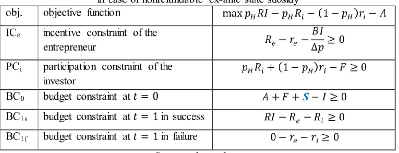
The only difference compared to the base case presented in Table 1 is that the budget constraint in 𝑡 = 0 is changed because also the state subsidy is involved in the project financing.
Table 3: The optimization program of the entrepreneur in case of nonrefundable ex-ante state subsidy
obj. objective function max 𝑝𝐻𝑅𝐼 − 𝑝𝐻𝑅𝑖− (1 − 𝑝𝐻)𝑟𝑖− 𝐴 ICe incentive constraint of the
entrepreneur 𝑅𝑒− 𝑟𝑒−𝐵𝐼
∆𝑝≥ 0 PCi participation constraint of the
investor
𝑝𝐻𝑅𝑖+ (1 − 𝑝𝐻)𝑟𝑖− 𝐹 ≥ 0
BC0 budget constraint at 𝑡 = 0 𝐴 + 𝐹 +𝑺− 𝐼 ≥ 0
BC1s budget constraint at 𝑡 = 1 in success 𝑅𝐼 − 𝑅𝑒− 𝑅𝑖 ≥ 0 BC1f budget constraint at 𝑡 = 1 in failure 0 − 𝑟𝑒− 𝑟𝑖≥ 0
Source: the authors
The optimization program can be solved again using the corresponding Lagrange function.
Similarly to the base case, all the constraints are binding. Applying Assumption 5 (No reward in failure) and the definitions of the pledgeable income (𝜌0) and of the present value of state subsidy (𝑆̅) Equations (14-18) can be derived. □
Proposition 2 (Entrepreneur accepts state subsidy) The entrepreneur will accept any of the subsidies presented in Table 2.
Proof The entrepreneur is supposed to be rational in the sense that he is maximizing his expected net benefit. According to Assumption 5 (No reward in failure), his total investment’s cash flow has only two elements: the investment of his initial asset (A) at the beginning and his return (𝑅𝑒) in case of success at 𝑡 = 1. Given that A is fixed (it is the maximum amount of asset he can invest at 𝑡 = 0), his only way to increase his net benefit is to increase his return in success which according to Equation (18) is the increasing function of the present value of state subsidy (𝑆̅). As the present value of the state subsidy is always nonnegative (𝑆̅ ≥ 0), the entrepreneur will accept it.□
14 Assumption 9 (State’s participation constraint) State has a participation constraint (PCS), as it cannot give out more subsidies than it is expected to return in form of quantifiable externalities appearing explicitly in the budget. In other words, the overall public utility of the subsidy cannot be negative between t=0 and t=1:
PCS 𝑈𝑝𝑢𝑏𝑙𝑖𝑐 = 𝑁𝑃𝑉𝑝𝑢𝑏𝑙𝑖𝑐 = 𝐸𝐼 − 𝑆̅ ≥ 0 (19)
It follows from Assumption 9 that the expected rate of return of the state is zero if both subsidies and externalities are also taken into account.
Proposition 3 (Optimum for nonrefundable ex-ante subsidy) There exists an optimal contract for a nonrefundable ex-ante subsidy:
- the size of the state subsidy is
𝑺 = 𝑺̅ = 𝑬
𝟏 − 𝝆𝟎 − 𝑬𝑨 (20)
- the size of the investment is
𝐼 = 1
1 − 𝜌0 − 𝑬𝐴 (21)
- the social utility is
𝑈 = 𝑝𝐻𝑅 + 𝐸 − 1
1 − 𝜌0 − 𝑬 𝐴 (22)
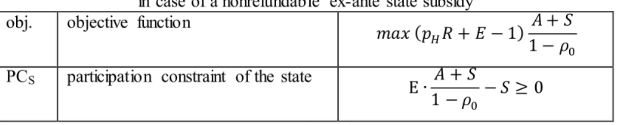
Proof The aim of the state is to maximize the social utility (𝑈) which is the sum of private and public benefits minus the total investment:
𝑚𝑎𝑥 𝑝𝐻𝑅𝐼 + 𝐸𝐼 − 𝐼 (23)
Substituting Equation (14) into (23) we get the objective function of the state with respect to the size of the state subsidy (in this special case 𝑆 = 𝑆̅)
𝑚𝑎𝑥 (𝑝𝐻𝑅 + 𝐸 − 1) 𝐴 + 𝑆 1 − 𝜌0
(24)
The state’s participation constraint formulated in Assumption 9 has also to be fulfilled.
Substituting Equation (14) into Inequality (19) we arrive at
PCS 𝐴 + 𝑆
1 − 𝜌0𝐸 − 𝑆 ≥ 0 (25)
15 Table 4 presents the states’ optimization program in case of a nonrefundable ex-ante state subsidy.
Table 4: The optimization program of the state in case of a nonrefundable ex-ante state subsidy obj. objective function
𝑚𝑎𝑥 (𝑝𝐻𝑅 + 𝐸 − 1) 𝐴 + 𝑆 1 − 𝜌0 PCS participation constraint of the state
E ∙ 𝐴 + 𝑆
1 − 𝜌0 − 𝑆 ≥ 0 Source: the authors
The optimization program can be solved by the Lagrange method, as usual. The constraint binds, in optimum p=pH, and we get Equations (20-22). □
3.3 Other forms of state subsidy
Other forms of state subsidy can also be examined in a similar way. Table 5 presents all the optimization programs in details, while Annex 2 summarizes the results.
Proposition 4 (Unconditional refundable subsidy has no effect) In case of subsidy form 4 (ex- ante subsidy refundable in any case) the subsidy does not influence the optimal project size and the social utility relative to the base case. If state intervenes in this form, it just crowds out private financing without any growth effect.
Proof When solving the corresponding optimization problem set out in Table 5 we get that the optimal project size is independent of the amount of the state subsidy and is equal to the project size in the case of two private players as in Equation (5):
𝐼 = 𝐴
1 − 𝑝𝐻(𝑅 − 𝐵∆𝑝)
= 1
1 − 𝜌0𝐴 (26)
Moreover, there are no separate formulae for the optimal size of the state subsidy (𝑆) and the private financing (𝐹), as they are prefect substitutes:
𝐹 + 𝑆 = 𝐼 − 𝐴 = 𝜌0
1 − 𝜌0𝐴 (27)
□ If the interest rate of the loan to be refunded is lower than the market rate, the interest rate subsidy can be expressed in its present value, and its effect is the same as that of a nonrefundable subsidy of a similar amount analyzed in section 3.2. As in the case of unconditionally refundable state subsidy the present value of the subsidy is zero, it does not
16 increase the initial asset of the entrepreneur in any sense; therefore it has no effect on the project size either.
Definition 2 (Real state subsidies) In case of subsidy forms 1, 2, 3, 5 and 6 the net present value of the subsidy (𝑆̅) is positive. Hence these schemes will be referred as real state subsidies, whereas form 4 will be excluded from the further investigations.
Proposition 5 (Neutrality of subsidy forms) In the optimums the net present value of the state subsidy (𝑆̅), the size of the investment (I), and the social utility (U) are the same for each real subsidy form. Hence the form of the state subsidy is irrelevant from macroeconomic perspective.
Proof Optimization programs in Table 5 can be solved by the Lagrange method. In case of all real subsidy forms constraints bind and a unique optimum can be easily derived as shown in Annex 2. □
17 Table 5: Optimization programs for different forms of state subsidies
1. Non-refundable ex-ante subsidy 2. Ex-post subsidy in success 3. Ex-post subsidy in failure
Step 1 max 𝑝𝐻𝑅𝐼 − 𝑝𝐻𝑅𝑖 − (1 − 𝑝𝐻)𝑟𝑖− 𝐴 max 𝑝𝐻(𝑅𝐼 + 𝑆) − 𝑝𝐻𝑅𝑖 − (1 − 𝑝𝐻)𝑟𝑖− 𝐴 max 𝑝𝐻𝑅𝐼 + (1 − 𝑝𝐻)𝑆 − 𝑝𝐻𝑅𝑖 − (1 − 𝑝𝐻)𝑟𝑖− 𝐴
ICe 𝑅𝑒− 𝑟𝑒− 𝐵𝐼
∆𝑝≥ 0 𝑅𝑒− 𝑟𝑒 −𝐵𝐼
∆𝑝≥ 0 𝑅𝑒 − 𝑟𝑒 − 𝐵𝐼
∆𝑝≥ 0 PCi 𝑝𝐻𝑅𝑖+ (1 − 𝑝𝐻)𝑟𝑖− 𝐹 ≥ 0 𝑝𝐻𝑅𝑖 + (1 − 𝑝𝐻)𝑟𝑖− 𝐹 ≥ 0 𝑝𝐻𝑅𝑖 + (1 − 𝑝𝐻)𝑟𝑖− 𝐹 ≥ 0
BC0 𝐴 + 𝐹 + 𝑆 − 𝐼 ≥ 0 𝐴 + 𝐹 − 𝐼 ≥ 0 𝐴 + 𝐹 − 𝐼 ≥ 0
BC1u 𝑅𝐼 − 𝑅𝑒 − 𝑅𝑖 ≥ 0 𝑅𝐼 + 𝑆 − 𝑅𝑒− 𝑅𝑖 ≥ 0 𝑅𝐼 − 𝑅𝑒− 𝑅𝑖 ≥ 0
BC1d 0 − 𝑟𝑒− 𝑟𝑖 ≥ 0 0 − 𝑟𝑒 − 𝑟𝑖≥ 0 𝑆 − 𝑟𝑒 − 𝑟𝑖 ≥ 0
Step 2 max 𝑝𝐻𝑅𝐼 + 𝐸𝐼 − 𝐼 max 𝑝𝐻𝑅𝐼 + 𝐸𝐼 − 𝐼 − 𝑝𝐻𝑆 max 𝑝𝐻𝑅𝐼 + 𝐸𝐼 − 𝐼 − (1 − 𝑝𝐻)𝑆
obj. max (𝑝𝐻𝑅 + 𝐸 − 1) 𝐴 + 𝑆
1 − 𝜌0 max (𝑝𝐻𝑅 + 𝐸 − 1)𝐴 + 𝑝𝐻𝑆
1 − 𝜌0 − 𝑝𝐻𝑆 max (𝑝𝐻𝑅 + 𝐸 − 1)𝐴 + (1 − 𝑝𝐻)𝑆
1 − 𝜌0 − (1 − 𝑝𝐻)𝑆 PCS
𝐸𝐼 − 𝑆 ≥ 0 𝐸𝐼 − 𝑝𝐻𝑆 ≥ 0 𝐸𝐼 − (1 − 𝑝𝐻)𝑆 ≥ 0
𝐸 𝐴 + 𝑆
1 − 𝜌0 − 𝑆 ≥ 0 𝐸𝐴 + 𝑝𝐻𝑆
1 − 𝜌0 − 𝑝𝐻𝑆 ≥ 0 𝐸𝐴 + (1 − 𝑝𝐻)𝑆
1 − 𝜌0 − (1 − 𝑝𝐻)𝑆 ≥ 0 4. Refundable ex-ante subsidy 5. Ex-ante subsidy refundable in failure 6. Ex-ante subsidy refundable in success Step 1 max 𝑝𝐻𝑅𝐼 − 𝑝𝐻𝑅𝑖 − (1 − 𝑝𝐻)𝑟𝑖− 𝐴 max 𝑝𝐻𝑅𝐼 − (1 − 𝑝𝐻)𝑆 − 𝑝𝐻𝑅𝑖 − (1 − 𝑝𝐻)𝑟𝑖− 𝐴 max 𝑝𝐻𝑅𝐼 − 𝑝𝐻𝑅𝑖 − (1 − 𝑝𝐻)𝑟𝑖− 𝑝𝐻𝑆 − 𝐴
ICe 𝑅𝑒− 𝑟𝑒− 𝐵𝐼
∆𝑝≥ 0 𝑅𝑒− 𝑟𝑒 −𝐵𝐼
∆𝑝≥ 0 𝑅𝑒 − 𝑟𝑒 − 𝐵𝐼
∆𝑝≥ 0 PCi 𝑝𝐻𝑅𝑖+ (1 − 𝑝𝐻)𝑟𝑖− 𝐹 ≥ 0 𝑝𝐻𝑅𝑖 + (1 − 𝑝𝐻)𝑟𝑖− 𝐹 ≥ 0 𝑝𝐻𝑅𝑖 + (1 − 𝑝𝐻)𝑟𝑖− 𝐹 ≥ 0
BC0 𝐴 + 𝐹 + 𝑆 − 𝐼 ≥ 0 𝐴 + 𝐹 + 𝑆 − 𝐼 ≥ 0 𝐴 + 𝐹 + 𝑆 − 𝐼 ≥ 0
BC1u 𝑅𝐼 − 𝑅𝑒 − 𝑅𝑖 − 𝑆 ≥ 0 𝑅𝐼 − 𝑅𝑒− 𝑅𝑖 ≥ 0 𝑅𝐼 − 𝑅𝑒− 𝑅𝑖− 𝑆 ≥ 0
BC1d 0 − 𝑟𝑒− 𝑟𝑖− 𝑆 ≥ 0 0 − 𝑟𝑒− 𝑟𝑖− 𝑆 ≥ 0 0 − 𝑟𝑒 − 𝑟𝑖 ≥ 0
Step 2 max 𝑝𝐻𝑅𝐼 + 𝐸𝐼 − 𝐼 max 𝑝𝐻𝑅𝐼 + 𝐸𝐼 − 𝐼 max 𝑝𝐻𝑅𝐼 + 𝐸𝐼 − 𝐼
obj. max (𝑝𝐻𝑅 + 𝐸 − 1) 𝐴
1 − 𝜌0 max (𝑝𝐻𝑅 + 𝐸 − 1)𝐴 + 𝑝𝐻𝑆
1 − 𝜌0 max (𝑝𝐻𝑅 + 𝐸 − 1)𝐴 + (1 − 𝑝𝐻)𝑆 1 − 𝜌0 PCS
𝐸𝐼 − 𝑆 + 𝑆 ≥ 0 𝐸𝐼 − 𝑆 + (1 − 𝑝𝐻)𝑆 ≥ 0 𝐸𝐼 − 𝑆 + 𝑝𝐻𝑆 ≥ 0
𝐸 𝜌0
1 − 𝜌0(𝐴 + 𝑆) − 𝑆 + 𝑆 ≥ 0 𝐸𝐴 + 𝑝𝐻𝑆
1 − 𝜌0 − 𝑆 + (1 − 𝑝𝐻)𝑆 ≥ 0 𝐸𝐴 + (1 − 𝑝𝐻)𝑆
1 − 𝜌0 − 𝑆 + 𝑝𝐻𝑆 ≥ 0 Source: the authors
18 4 Results
In this section we compare and analyze the results of the optimization programs presented in Table 5. The most important result is that all real subsidies increase social welfare compared to the base case.
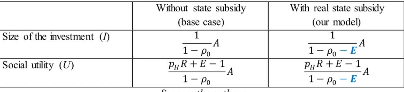
Proposition 6 (Value added of real state subsidies) Real state subsidies unambiguously create value which is reflected in the increased project size and social utility.
Proof In case of the basic two-player model the social utility (U) is 𝑈 = 𝑝𝐻𝑅 + 𝐸 − 1
1 − 𝜌0 𝐴 (28)
which comes from the combination of Equations (5) and (11) using that in optimum p=pH. In order to keep the model close to the reality we supposed the positivity of the investment size (𝐼 > 0) and the present value of state subsidy (𝑆 > 0), as well. It follows from these assumptions and from Equation (17) that in the optimum 1 − ρ0 − E > 0. Provided that Assumption 1 (Unconditional positive externalities) also holds, the comparison of Equation (5) to Equation (21) and Equation (28) to Equation (22) will lead us to the conclusion that in the optimum the size of the investment and also the social utility are unambiguously increased due to the state subsidy as it is summarized in Table 6:
Table 6: Comparison of the results in the optimum Without state subsidy
(base case)
With real state subsidy (our model)
Size of the investment (I) 1
1 − 𝜌0𝐴 1
1 − 𝜌0− 𝑬𝐴
Social utility (U) 𝑝𝐻𝑅 + 𝐸 − 1
1 − 𝜌0 𝐴 𝑝𝐻𝑅 + 𝐸 − 1 1 − 𝜌0− 𝑬 𝐴 Source: the authors
□ Therefore, it has been demonstrated that contrary to the common believes a properly designed subsidy system does not worsen, but improves the contractual incentives, so it effectively reduces moral hazard. The reduction in moral hazard can be due to the direct effect of additional capital provided by the state; but also to the indirect effect of the state capital to mobilize more private capital. Besides moral hazard, the state subsidy effectively resolves another market failure, as well: the externalities. Without state subsidy, these potential benefits are lost for the society.
As we can see in Table 9 in Annex 2, in the optimum, the net present value of state subsidy (𝑆̅) is the same for all real subsidy forms, and its size depends only on the externalities (𝐸), on the pledgeable income (ρ0) and the initial asset of the entrepreneur (𝐴).
19
𝑆̅ = 𝐸
1 − 𝐸 − 𝜌0𝐴 (29)
Hence, the same amount of public money induces the same project size and the same level of social welfare. Thus, these subsidy forms differ only in their phrasing and their internal structure, but their growth effects are the same. As the net present value of the state subsidy is the same, different forms of subsidies only influence the cash-flow of the private investor (F, Ri, ri).
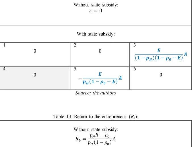
Interestingly, the cash-flow of the entrepreneur (Re) remains always the same, see Table 13 in Annex 2. Therefore, we can conclude that one important role of the private investor (besides providing the necessary capital) is to transform the cash-flow of the state subsidy into the shape what is optimal from the moral hazard aspect.
For example in subsidy form 3 (ex post subsidy in case of failure or state guarantee) state only provides rescue in failure. However, according to Assumption 5 the entrepreneur cannot receive any transfer in failure (that would destroy his incentives); therefore it must be the private investor who receives this money directly. But, as this additional safety belt is provided by the state, the private investor is willing to provide more financing at the beginning in t=0 which makes the project size larger with all its beneficial effects.
Another interesting case is subsidy form 5 (ex-ante subsidy refundable only in failure). It is clear that the entrepreneur is not able to pay anything in case of failure on his own as he has already invested all his capital into the project and has a limited liability. Therefore, in case of failure it is the private investor who has to stand in the gap and fulfill the commitment toward the state.10
It is worth to examine the optimal level of private financing (𝐹), as well. If it is decreased relative to the base case, then it can be considered as the sign of some crowding out effects of the state subsidy.
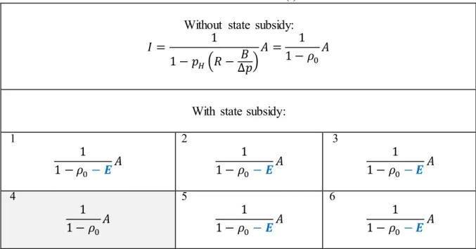
Proposition 7 (Crowding out effect) Nonrefundable state subsidies (1, 2, 3) do not crowd out private investors; moreover, they boost private financing by providing additional capital, hence reducing moral hazard. The same is true for conditional refundable subsidy form 6, but form 5 may crowd out private financing depending on the parameter setting. Unconditional refundable subsidy (4) has no other effect but crowding out.
Proof We can see in Table 10 in Annex 2 that the optimal private financing (𝐹) takes different values under different subsidy forms. In case of subsidy forms 1, 2, and 3 it is obvious for the first sight that state subsidy increases private financing as denominators are decreased and numerators are increased (forms 2, 3) or did not change (form 1).
10 Apart from these two cases the return to the private investor in failure (ri) equals zero similarly to the basic two-player case.
20 In case of subsidy form 6 private financing is increased if and only if
𝜌0− 𝒑𝟏 − 𝒑𝑯 𝑯𝑬
1 − 𝜌0 − 𝑬 𝐴 > 𝜌0 1 − 𝜌0𝐴
(30)
Given that both denominators are positive, it follows that Inequality (30) is equivalent to 𝜌0 > 𝑝𝐻. This always holds since Inequality (13) implies (𝑝𝐻− 𝑝𝐿)𝑅 > 𝐵.
In case of subsidy form 5 we similarly obtain that there is no crowding out effect if and only if 𝜌0 > 1 − 𝑝𝐻. This inequality holds if 𝑝𝐻 > 0.5 or 𝑝𝐻𝑅 > 2 or 𝐵 > 𝑝𝐻 − 𝑝𝐿, but can befalse for suitable parameter settings, for example 𝐸 = 0.1, 𝑅 = 2.6, 𝑝𝐻 = 0.4, 𝑝𝐿 = 0.25, and 𝐵 = 0.2.
As far as unconditional refundable subsidy is concerned, its crowding out effect was extensively discussed in Proposition 4. □
As we saw, it is only form 5 which may have a crowding out effect in the sense that the initial private investment can be lower than in the base case. This is due to the fact that form 5 is the only one where private investor has to contribute not only at the beginning of the project but also at the end in case of failure. A simple calculation shows that if we added also the expected value of these expenses to the initial investment, then there would be no crowding out effect for this form either.
Proposition 8 (Entrepreneur gets all surpluses) In the three-player moral hazard model the total social surplus is given to the entrepreneur which motivates him to exert maximum effort.
Proof The entrepreneur invests 𝐴 at 𝑡 = 0 and gets back 𝑅𝑒 in case of success and nothing in case of failure. His return in success (𝑅𝑒) is the same under each real subsidy form; see Table 13 in Annex 2. His net surplus (𝑁𝑃𝑉𝑒) can be expressed as
𝑁𝑃𝑉𝑒 = 𝑝𝐻𝑅𝑒 − 𝐴 = 𝑝𝐻 𝑝𝐻𝑅 − 𝜌0
𝑝𝐻(1 − 𝜌0− 𝑬)𝐴 − 𝐴 = 𝑝𝐻𝑅 + 𝐸 − 1 (1 − 𝜌0 − 𝑬)
which is just the total social utility given in Table 14 in Annex 2. □
We remind that in the base case model only the private surplus was given to the entrepreneur, whilst the positive external effects were enjoyed by the broader society for free. In our three player model the positive external effects are increased significantly due to the state subsidy (see Proposition 6); moreover, the society pays out all of these externalities to the entrepreneur. Hence, in the end of the story externalities became internalized.
21 5 Conclusions
In order to model the relationship between state subsidy and moral hazard in corporate financing we built on the seminal paper of Holmström and Tirole (1997) which is considered as one of the best representations of the topic in case of private parties (entrepreneur and private investor). We kept all the assumptions of this basic model (sizeable project with constant rate of return, relevance of moral hazard, risk neutrality of both private players, limited liability of the entrepreneur, unlimited liability of the investor, no reward for the entrepreneur in failure), but generalized it by introducing state as a third player. As a strict budget constraint, state could only finance the subsidies from the positive externalities realized by the end of the project.
It can be concluded from our investigation that negative experiences with subsidized projects cannot be explained by the mere fact of state subsidy. In the framework of our model moral hazard is decreased, the size of the project is increased, and social welfare is definitely improved by the state intervention; and it is independent from the form of the state subsidy (provided that it is considered as a real subsidy).
Moreover, in case of nonrefundable subsidies (forms 1, 2, and 3) state does not crowd out private investors; but on the contrary, by providing additional capital it boosts private financing. Refundable subsidies show a mixed picture. Non-subsidized loans to be refunded unconditionally in any case (both in success and failure) have no growth effects at all, and state subsidy crowds out private investments completelyhence this is definitely not an appropriate tool to fight credit rationing and moral hazard. Ex-ante subsidies refundable only in success (form 6) has no crowding out effect at all, whereas ex-ante subsidies refundable only in failure (form 5) may or may not crowd out depending on the parameters.
It is also remarkable that in the optimum it is the entrepreneur who gets all the private and social surplus of the project, which constitutes a strong motivation for him to exert high efforts for the success of the project. Hence, as a result of state intervention externalities become internalized by the private parties; which contributes to the efficiency at macro level, as well.
Of course, in the real world it is not guaranteed that state makes optimal contracts. For example it may subsidize projects without any positive social effect, and/or may serve the interest of particular lobbies, and/or incentives are not properly set because of lack of information, and/or administration is too costly etc. However, as we have proven, the moral hazard experienced in subsidized projects is not due to the state subsidy per se. Further research can clarify which aspects are responsible for these unfavorable phenomena.
22 Annex 1: Empirical literature
Table 7: Summary of empirical literature on state subsidies
Authors Year of publ.
Database Moral hazard / adverse selection
Other effects of state subsidy
Overall effect
Crowding out 1 Biagi,
Martini
2015 Italy 2000-2009
effects differ across regions within the same country
positive
2 Bondonio, Greenbaum
2010 Italy 2000-2003
higher leverage positive
3 Borisova et al.
2015 43 countries 1991-2010
moral hazard (higher risk, less efficiency)
positive in crisis and in case of high-bankruptcy risk firms
positive only in crisis
4 Breska (page 209)
2010 East Germany 1996-2007
enhanced investment positive
5 Bronzini, Piselli
2016 Italy 2005-2011
moral hazard in case of larger firms
positive in case of SMEs 6 Cull et al. 2015 China
2000-2002
firms easier to overcome market failures with governmental aid
positive
7 Czarnitzki, Lopes-Bento
2013 Flanders (Belgium) 2002-2008
repeated support does not decrease efficiency
positive no
8 Garcia, Mohn
2010 Austria 1998-2000
boosted R&D spending positive
9 Girma, Görg, Strobl
2007 Ireland 1992-1998
additional financing, improves productivity more for capital constrained firms
positive
10 González, Pazó
2008 Spain 1990-1999
no adverse selection
more innovation positive no
11 Hong et al. 2015 China 1995-2008
moral hazard in case of larger high-tech firms
positive no
12 Huergo,
Moreno 2014 Spain
2002-2005 more patents and product
innovations positive
13 Huergo, Trenado, Ubierna
2015 Spain 2002-2005
adverse selection (larger firms overrrepresented)
more R&D, persistence in R&D spending
positive in case of SMEs 14 Kállay 2014 Hungary
2004-2011
moral hazard negative
23
15 Luukkonen, Deschryvere, Bertoni
2013 7 EU countries 1994-2004
no moral hazard in case of gov.
venture funds
state owned venture fund adds value in a different way than privately owned ones
positive (similar to private VC) 16 Meuleman,
Maeseneire
2012 Belgium 1995-2004
reduced adverse selection
better long term financing possibilities
positive
17 Monqué 2012 EU
countries, review of other studies
easing shortage of capital, low efficiency in larger firms
positive only in case of SMEs 18 Simachev,
Kuzyk, Feygina
2015 Russia 2012
adverse selection, moral hazard
grant for innovation only boosts export
not significant
yes
19 Widerstedt, Månsson
2015 Sweden 2004-2007
adverse selection faster growth but no efficiency improvement
low or no added value
yes
20 Zheng, Zhu 2013 China 1999-2005
moral hazard in case of firms with political support
debt of firms with strong political connections less linked to profitability
unclear
Source: the authors