BIOSTATISTICS
A first course in probability theory and statistics for biologists
J´ anos Izs´ ak, Tam´ as Pfeil
2013.10.6
Contents
Preface 4
I Probability theory 7
1 Event algebra 8
1.1 Experiments, sample space . . . 8
1.2 Events . . . 10
1.3 Operations on events . . . 11
1.4 Event algebra . . . 15
2 Probability 17 2.1 Relative frequency, probability . . . 17
2.2 Probability space . . . 19
2.2.1 Classical probability spaces . . . 19
2.2.2 Finite probability spaces . . . 22
2.2.3 Geometric probability spaces . . . 23
2.3 Some simple statements related to probability . . . 25
3 Conditional probability, independent events 27 3.1 Conditional probability . . . 27
3.2 The product rule . . . 29
3.3 The total probability theorem . . . 29
3.4 Bayes’ theorem . . . 31
3.5 Independent events . . . 33
3.6 Independent experiments . . . 35
3.7 Exercises . . . 37
4 Random variables 41 4.1 Random variables . . . 41
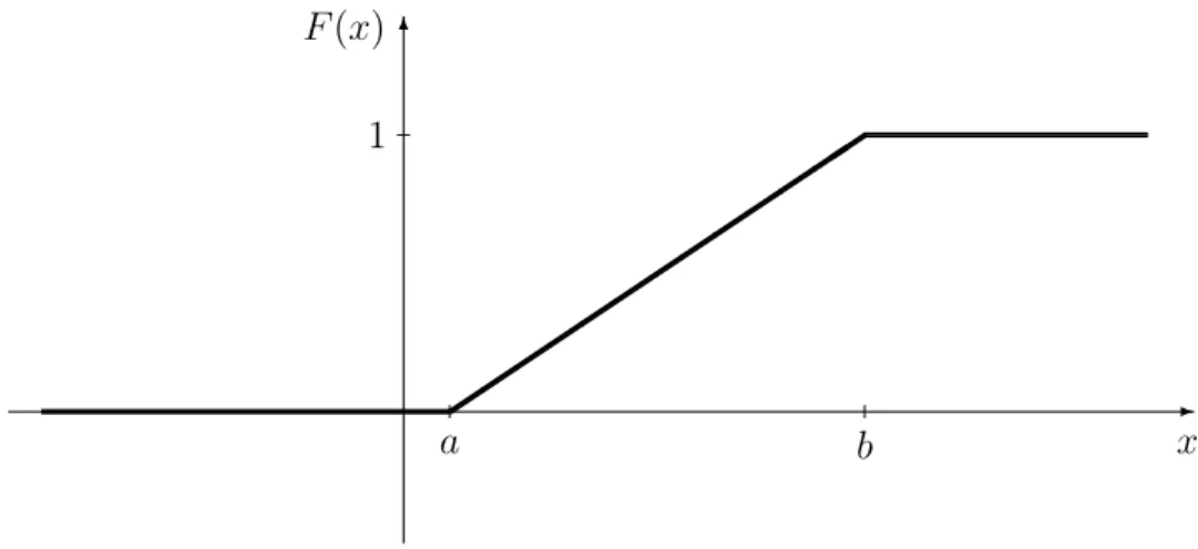
4.2 The distribution function . . . 42
4.3 Independent random variables . . . 45
4.4 Discrete random variables . . . 45
4.5 Continuous random variables . . . 46
4.6 Empirical distribution function, density histogram . . . 48
4.7 Expected value . . . 50
4.8 Further quantities characterizing the mean of random variables . . . 53
4.9 Variance . . . 54
5 Frequently applied probability distributions 57 5.1 Discrete probability distributions . . . 57
5.1.1 The discrete uniform distribution . . . 57
5.1.2 The binomial distribution . . . 58
5.1.3 The hypergeometric distribution . . . 59
5.1.4 Poisson distribution . . . 60
5.1.5 The geometric distribution . . . 62
5.1.6 The negative binomial distribution . . . 63
5.2 Continuous distributions . . . 63
5.2.1 The continuous uniform distribution . . . 63
5.2.2 The normal distribution . . . 64
5.2.3 The lognormal distribution . . . 68
5.2.4 The chi-squared distribution . . . 68
5.2.5 The t-distribution . . . 68
5.2.6 The F-distribution . . . 69
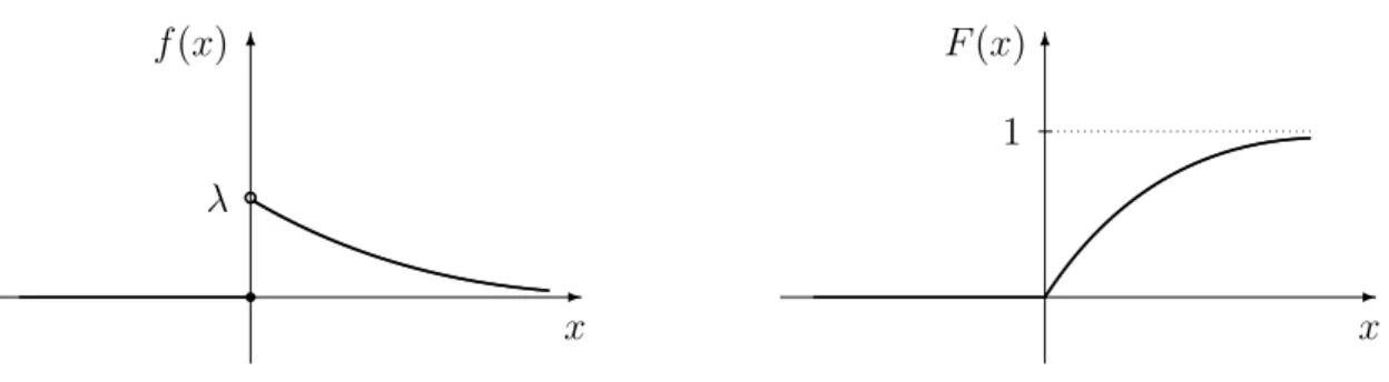
5.2.7 The exponential distribution . . . 69
5.2.8 The gamma distribution . . . 70
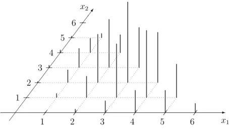
6 Random vectors 71 6.1 Some concepts related to the multivariate, specifically bivariate distributions 73 6.2 Stochastic relationship between the components of a random vector . . . 75
6.2.1 Covariance and linear correlation coefficient . . . 75
6.2.2 Rank correlation coefficients . . . 77
6.3 Frequently used multivariate or multidimensional distributions . . . 79
6.3.1 Polynomial or multinomial distribution . . . 79
6.3.2 Multivariate hypergeometric distribution . . . 80
6.3.3 Multivariate or multidimensional normal distribution . . . 80
6.3.4 The regression line . . . 80
7 Regression analysis 83
II Biostatistics 87
Introduction 88
8 Estimation theory 89
8.1 Point estimation of the expected value and the variance . . . 89
8.2 Interval estimations, confidence intervals . . . 92
8.2.1 Confidence interval for the expected value of a normally distributed random variable with unknown standard deviation . . . 92
8.2.2 Confidence interval for the probability of an event . . . 96
8.2.3 Point estimation for the parameters of the linear regression . . . . 98
8.2.4 Point estimations of the correlation coefficients . . . 104
9 Hypothesis testing 111 9.1 Parametric statistical tests . . . 118
9.1.1 One-sample t-test . . . 118
9.1.2 Two-sample t-test . . . 120
9.1.3 Welch-test . . . 123
9.1.4 F-test . . . 125
9.1.5 Bartlett’s test . . . 128
9.1.6 Analysis of variance (ANOVA). . . 129
9.2 Non-parametric statistical tests . . . 140
9.2.1 Hypothesis testing based on chi-squared tests . . . 140
10 Further statistical tests for the distribution and parameters of random variables 157 10.1 Kolmogorov test for checking the equality of a continuous distribution function and a known distribution function . . . 157
10.2 The Mann–Whitney test or Wilcoxon rank-sum test . . . 159
10.3 Kruskal–Wallis test . . . 161
11 Further tests on correlation 164 11.1 Testing whether the correlation coefficient is zero . . . 164
11.2 Fisher’s transformation method for testing the equality of two correlation coefficients . . . 166
11.3 Testing whether Spearman’s rank correlation coefficient is zero . . . 167
11.4 Testing whether Kendall’s rank correlation coefficient is zero . . . 167
A Statistical tables 169
Index 179
References 181
Preface
This coursebook is intended to serve the education of students of biology studying prob- ability theory and biostatistics.
During the mathematical education of students of biology, little time can be devoted to teaching the basics of probability theory. This fact in itself makes it necessary to discuss probability theory at some length before statistical studies. However, for students of biology a certain amount of knowledge of probability theory is also very important for its own sake, since a stochastic way of thinking and learning about stochastic models are indispensable in several fields of biology. To some extent all this refers to the statistics education of students of chemistry as well. According to what has been said, in the first part of the book the basics of probability theory are discussed in the framework of a material planned for about a semester. The second part of the book having approximately the same length is about mathematical statistics. We also aimed to provide a material that is completely learnable in two semesters. When writing the book, we relied on our educational experience obtained in several decades of teaching probability theory and biostatistics. In view of the knowledge and needs of the students, both parts have been illustrated with plenty of biological examples and figures.
The beginning part (basics of probability theory) and the continuation (multivari- ate probability theory, biostatistics) of this book are treated somewhat differently. The reason is that the beginning of the book, being part of the compulsory courses of mathe- matics for biology students, is the work of the second author, while the further chapters, being part of two optional third-year courses, are the work of the first author.
We thank the translator, ´Agnes Havasi, assistant lecturer for her thorough work and several stylistic advices, and ´Eva Valk´o, PhD student for the careful preparation of some of the figures.
We express our special thanks to M´arta Lad´anyi, associate professor (Corvinus Uni- versity, Budapest, Faculty of Horticultural Science, Department of Mathematics and Informatics) for her conscientious revision of the book and considerably large number of her valuable suggestions.
We thank Katalin Fried, associate professor for her help during the preparation of this book.
We appreciate if the Reader lets us know his/her potential critical remarks, sugges- tions for improvement or other comments.
Budapest, August, 2013. The authors
Part I
Probability theory
Chapter 1
Event algebra
Probability theory is concerned with the analysis of phenomena that take place in in- deterministic, in other words random circumstances. In this chapter we briefly discuss random events and experiments on random events.
1.1 Experiments, sample space
Natural phenomena can be classified into two groups. The first group contains those phenomena which take place in the same way, i.e., produce the same outcome under the same given conditions. These phenomena are called deterministic, and such are for example free fall and the day and night cycle.
In the other group of phenomena, the circumstances that are (or can be) taken into account do not determine uniquely the outcome of the phenomenon, i.e., the outcome cannot be predicted before the occurrence of the phenomenon. These are called random (or stochastic) phenomena. A random phenomenon can either be created by us or ob- served. An example for the former one is the roll of a die, and for the latter one the determination of the height of a randomly chosen person. In the sequel we will only consider random phenomena which occur frequently or can be repeated several times, in industrial applications these are called random mass phenomena. Random phenomena may result in several different outcomes, however, the attribute ”random” does not mean that the outcome has no cause, it only means that we cannot or do not wish to take into account all the existing circumstances.
An observation or (random) experiment regarding a random event results in a so- called elementary event. The set of the possible elementary events will be referred to as sample space and denoted by Ω. If the outcome of the experiment is the elementary event ω, then we can say that ω occurs in the given experiment.
During each experiment, i.e., each time the studied random phenomenon occurs, the outcome is one of the possible outcomes, or, to put it differently, exactly one elementary
event occurs. Some subsets of the sample space are the so-called (observable) events, see below.
Example 1.1. (a) Roll of a die. A die is a cube with its six faces showing1, 2, 3, 4, 5 and 6 dots. Let the experiment be as follows: we roll a die, and when it has fallen down we observe the number of dots on its upper face. We define six outcomes or elementary events, namely:
ω1 :=the roll is a 1, ω2 :=the roll is a 2, ω3 :=the roll is a 3, ω4 :=the roll is a 4, ω5 :=the roll is a 5, ω6 :=the roll is a 6.
So, the sample space has six elements, Ω ={ω1, ω2, ω3, ω4, ω5, ω6}.
(b) During the experiment we roll the die mentioned in the previous point, but now we only register if the number of dots on the upper face is even or odd. The observed outcomes are:
˜
ω1 :=the roll is an even number, ω˜2 :=the roll is an odd number.
In this experiment the sample space has two elements, Ω =˜ {ω˜1,ω˜2}.
(c) Coin flipping. We flip a coin, and when it has fallen down, we examine which side is facing up (heads or tails). This experiment has two possible outcomes:
h:=the face-up side is head, t :=the face-up side is tail.
The sample space has again two elements, Ω = {h, t}.
(d) Let the experiment be that we place an insect trap, and in an hour’s time we examine whether it has caught any specimen of three studied species (A, B, C). The sample space can be
Ω :={∅,{A},{B},{C},{A, B},{A, C},{B, C},{A, B, C}},
where, e.g., {A, C} denotes that in the trap there are specimens from species Aand C, but not from species B. The sample space is the power set of the set containing the three species {A, B, C}, and it consists of9 elements.
1.2 Events
During an experiment we are mostly unable to observe and at the same time uninterested in exactly which elementary event is the outcome.
By event (or observable event) we mean certain subsets of the sample space Ω. So every event is a set of elementary events.
Two notable events are thecertain event (Ω) and theimpossible event (∅).
Example 1.2. In the case of the coin flip the sample space Ω = {h, t} has the subsets
∅, {h}, {t}, Ω, which can be taken for (observable) events.
We will need some further notions related to events.
In a given experiment an eventoccurs if the outcome of the experiment is any of the elementary events corresponding to the given event.
The certain event occurs when any elementary event of the set Ω occurs. Since this happens any time that the experiment is performed, the certain event always (i.e.,
”certainly”) occurs.
The impossible event occurs when an elementary event belonging to the empty set occurs. The empty set has no elements, so the impossible event never occurs when the experiment is performed. This explains its name.
Example 1.3. In the example of rolling a die:
E1 :=the roll is an even number that is greater than 2, E2 :=the roll is at least a 4, but not a 5,
E3 :=the roll is a 4 or a 6.
The above three events are identical, or in other words, equal, since all occur when we roll a 4 or a 6. That is, E1 =E2 =E3 ={4,6}.
This example also shows that the same event can be formulated in different ways.
We say that the occurrence of event E implies the occurrence of event F if in each experiment where E occurs F also occurs. Since every event is a set of elementary events, this means that every elementary event in E is an element of event F as well, i.e., E is a subset of F. Therefore, if the occurrence of E implies the occurrence of F, the notation E ⊂F is used.
Two events are mutually exclusive if they cannot occur at the same time. A finite set of events are called pairwise mutually exclusive if no two of the elements can occur at the same time. A finite set of events form a complete set of events if they are pair- wise mutually exclusive, and one of them definitely occurs any time the experiment is performed.
Example 1.4. Consider the roll of a die.
(a) Mutually exclusive events are
E1 :=the roll is an even number, E2 :=the roll is a 1.
(b) Pairwise mutually exclusive events are
E1 :=the roll is an even number, E2 :=the roll is a1, E3 :=the roll is a 3.
(c) The following events form a complete set of events:
E1 :=the roll is an even number, E2 :=the roll is a 1, E3 :=the roll is a 3, E4 :=the roll is a 5.
1.3 Operations on events
We know the union, intersection and difference of sets and the complement of a set. Since events are certain subsets of the sample space, we can perform set operations on them.
The notations conventionally used for events differ from the corresponding notations of set theory. At the end of this chapter we give the set-theoretic analogues of all operations with notations.
If an event of the sample space Ω isE ⊂Ω, then thecomplement oropposite of event E is the event that occurs when E does not occur. Notation: E.
The complement of the certain event is the impossible event, and the complement of the impossible event is the certain event, i.e., Ω =∅ and ∅= Ω.
Set operations are commonly illustrated by Venn diagrams, therefore we will also use them for operations on events. Let the sample space be a rectangle Ω, and let the experiment be choosing a point of this rectangle. The complement of event E ⊂Ω is the difference Ω\E, since the complement event means choosing a point which belongs to Ω, but does not belong to E (see Fig. 1.1).
Further operations on events will also be illustrated on this experiment.
Example 1.5. In the example of rolling a die:
E :=the roll is an even number, E =the roll is an odd number, F :=the roll is a 6, F =the roll is a 1, 2, 3, 4 or 5.
Ω
E E
Figure 1.1: Complement of an event.
For a given sample space, any event and its complement (E, E) form a complete set of events consisting of two events, that is to say Ω = E∪E.
IfE andF are events in the same sample space, then thesum of E and F is defined as the event that occurs when event E or event F occurs. Notation: E +F (see Fig.
1.2).
In the definition of the sum the connective or is understood in the inclusive sense, i.e., the sum of two events can occur in three ways: either E occurs and F does not occur, or F occurs and E does not occur, or both occur. That is to say E+F occurs if at least one of event E and event F occurs.
Ω
E
F E+F
Figure 1.2: The sum of events.
We can formulate this more generally: ifE1, E2, . . . , Enare events in the same sample space, then let their sum be the event that occurs when any one of the listed events occurs.
Notation:
n
P
i=1
Ei or E1+. . .+En.
IfE1, E2, . . . form an infinite sequence of events in the same sample space, then their sum is defined as the event that occurs when any one of the listed events occurs. Notation:
∞
P
i=1
Ei orE1+E2+. . .
IfE and F are events in the same sample space, then theirproduct is the event that occurs when both events occur. The product is denoted by E ·F or, briefly, EF (see Fig. 1.3).
Ω
E
F EF
Figure 1.3: The product of events.
IfE1, . . . , Enare events in the same sample space, then let their product be the event that occurs when all the listed events occur. Notation:
n
Q
i=1
Ei orE1·. . .·En.
The events E and F are mutually exclusive if and only if EF =∅, since both mean that the two events cannot occur at the same time.
IfE andF are events in the same sample space, then thedifference of these events is defined as the event that occurs when E occurs, but F does not occur. Notation: E−F (see Fig. 1.4).
Example 1.6. In the example of rolling a die:
E :=the roll is an even number,
F :=the roll is a number that is smaller than 3, then
E+F = the roll is an even number or a number that is smaller than 3
= the roll is a 1, 2, 4 or 6,
Ω
E
F E−F
Figure 1.4: The difference of events.
EF =the roll is an even number and its value is smaller than 3 =the roll is a 2, E−F = the roll is an even number and its value is not smaller than 3
= the roll is a4 or a6.
In the following table we list the operations on events and the corresponding opera- tions on sets:
Operations on events, notations: Operations on sets, notations:
complement, E sum, E+F product, EF difference, E−F
complement, Ec union, E∪F intersection, E∩F difference, E\F
If E1, E2, . . . , En form a finite sequence of events in the same sample space, then the related de Morgan’s laws read as
E1+. . .+En =E1·. . .·En, E1·. . .·En=E1+. . .+En.
Example 1.7. In a study area three insect species (A, B, C) can be found. We place an insect trap, and after some time we look at the insects that have been caught. Let
E1 :=a specimen of species A can be found in the trap, E2 :=a specimen of species B can be found in the trap, E3 :=a specimen of species C can be found in the trap.
By using the events E1, E2, E3 and the operations, we give the following events:
(a) There is no specimen of species A in the trap=E1. There is no specimen of species B in the trap=E2. There is no specimen of species C in the trap=E3. (b) There is no insect in the trap=E1 E2 E3.
(c) There is an insect in the trap=E1+E2+E3.
(d) There are only specimens of a single species in the trap =E1 E2 E3+E1 E2 E3+ E1 E2 E3.
(e) There are specimens of two species in the trap=E1 E2 E3+E1 E2 E3+E1 E2 E3. (f ) There are specimens of all the three species in the trap=E1E2E3.
(g) Application of de Morgans’ law: There are specimens of at most two species in the trap. (There are no specimen or are specimens of one or two species but not of all the three species in the trap.) E1E2E3 =E1+E2+E3.
1.4 Event algebra
In an experiment we can choose the set of events within certain bounds. Every event in such a set of events should be observable, that is we should be able to decide whether the given event has occurred during the experiment. On the other hand, the set of events should be sufficiently large so that we can mathematically formulate all questions that arise in connection with the experiment. If the sample space consists of an infinite number of elementary events, then it can cause mathematical difficulties to assign a probability function to the set of events that is in accordance with our experiences.
We require that the results of the operations performed on the events (complement, sum, product, difference) are themselves events. To put this requirement differently, the set of events should be closed with respect to the operations. Moreover, we would like the certain event and the impossible event to be indeed events. In the general case we do not demand that subsets of the sample space with exactly one element be events. Our expectations for the set of events are satisfied by the following so-called event algebra.
If Ω is the sample space, then a set A, consisting of certain subsets of Ω, is an event algebra if the following three statements hold:
(a) Ω∈ A.
(b) For all E ∈ A,E ∈ A.
(c) If for all i∈N+,Ei ∈ A, then
∞
P
i=1
Ei ∈ A.
An event algebra with the above three properties is called a sigma algebra.
Chapter 2 Probability
In this chapter first we introduce the notion of relative frequency. With the help of this, we define the intuitive notion of probability, which will be followed by its axiomatic introduction. Then we deal with probability spaces, and, finally, summarize the basic relations that are valid for probability.
2.1 Relative frequency, probability
When an experiment is performed ”independently” several times, we talk about asequence of experiments. The independent execution of the experiments intuitively means that the outcome of any execution of the experiment is not influenced by the outcome of any other execution of the experiment. For example, when flipping a coin or rolling a die, the thrown object should rotate sufficiently many times so that its earlier position does not influence noticeably the outcome of the given toss. Later we will exactly define what is meant by the independent execution of the experiments (see Section 3.6).
Let us perform the experimentn times independently, and observe how many times a given event E occurs. Let us denote this number byk (or kE), and call it thefrequency of event E.
The ratio nk shows in what proportion eventE has occurred during the n executions of the experiment. This ratio is called the relative frequency of event E.
Example 2.1. When flipping a coin, let us use the notationhif after the flip the face-up side is ”head”, and the notation t if after the flip the face-up side is ”tail”. We flip a coin 20 times one after the other ”independently”, and let the finite sequence of outcomes be
t t h t h t t h t t h t h h h t h h t t.
The frequency of the side ”head” is 9, and its relative frequency is 209 = 0.45. Denote the frequency of the side ”head” in the nth flip by kn, then its relative frequency is knn, where
n = 1,2, . . . ,20. The 20-element finite sequence of relative frequencies of the side ”head”
in the above sequence of experiment is 0
1, 0 2, 1
3, 1 4, 2
5, 2 6, 2
7, 3 8, 3
9, 3 10, 4
11, 4 12, 5
13, 6 14, 7
15, 7 16, 8
17, 9 18, 9
19, 9 20. Example 2.2. The following three sequences of experiments on coin flips are also inter- esting from a historical point of view. The results of the experiments are given in Table 2.1.
name of experimenter, number of frequency relative frequency year of birth and death flips of heads of heads
Georges Buffon (1707-1788) 4040 2048 0.5080
Karl Pearson (1857-1936) 12000 6019 0.5016
Karl Pearson (1857-1936) 24000 12012 0.5005 Table 2.1: Data of three sequences of experiments on coin flips.
On the basis of our experiences obtained in the experiments theprobability of an event can intuitively be given as the number around which the relative frequencies oscillate.
In problems arising in practice, we do not usually know the probability of an event. In such a case, for want of anything better, the relative frequency obtained during a consid- erably large sequence of experiments can be considered as the (approximate) probability of the given event.
The above notion of probability is only intuitive because in it we find the undefined notion of the oscillation of relative frequencies.
LetA be an event algebra on the sample space Ω. The function P: A →R is called probability function if the following three statements are satisfied:
(a) For all events E ∈ A,P(E)≥0.
(b) P(Ω) = 1.
(c) If for all i ∈ N+, Ei ∈ A, moreover, if E1, E2, . . . form a sequence of pairwise mutually exclusive events, then P
∞ P
i=1
Ei
=
∞
P
i=1
P(Ei).
(So, in the case of a(n infinite) sequence of pairwise mutually exclusive events, the probability that one of the events occurs is equal to the sum of the (infinite) series of the probabilities of the events. This is calledsigma additivity ofP, where
’sigma’ is for ’infinite’.)
If E ∈ A is an event, then the number P(E) assigned to it is called the probability of event E.
Condition (c) can be applied also for a finite sequence of pairwise mutually exclusive events. That is to say, if with condition (c)P(En+1) = P(En+2) =. . .= 0 holds, then we get that for pairwise mutually exclusive eventsE1, . . . , En,P
n P
i=1
Ei
=
n
P
i=1
P(Ei). This is what we call the additivity of probability function. If n = 2, then for two mutually exclusive events E1 and E2 the above condition yields P(E1+E2) =P(E1) +P(E2).
If the sample space is finite, then the sequence of events in condition (c) is the impossible event with a finite number of exceptions. Therefore, in a finite sample space sigma additivity is identical to the additivity of function P.
In the definition of probability the requirements (a), (b) and (c) are called Kol- mogorov’s axioms of probability. All statements valid for probability can be derived from these axioms.
2.2 Probability space
The triplet of a given sample space Ω, the event algebra A consisting of certain subsets of Ω and the probability function P defined on the event algebraA is calledKolmogorov probability space (or probability space), and is denoted as (Ω,A, P).
In the case of an experiment, the sample space Ω consists of the possible outcomes of the experiment. The choice of the event algebra is our decision. It is worthwhile to choose one which consists of observable events and which allows us to formulate all arising problems, but it should not be too large, which would cause mathematical difficulties in the definition of the probability function. The probabilities of the events should be defined in accordance with our experience.
There are different possibilities to assume a probability function for a given sample space and event algebra. For example, in the case of rolling a die there can be different probabilities when the die is fair and when it has an inhomogeneous mass distribution.
In the following, we present some frequently encountered types of probability spaces.
2.2.1 Classical probability spaces
Several experiments have a finite number of outcomes, and in many cases we can notice that all outcomes have the same chance of occurring. This is the case when we flip a coin or roll a die, provided that the coin has the shape of a straight cylinder and a homogeneous mass distribution, and the die has the shape of a cube and also has a
homogeneous mass distribution. Such a coin or cube is called fair. The so-called classical probability space is created with the aim of describing experiments of this kind.
The triplet (Ω,A, P) is called classical probability space if the sample space Ω is a finite set, with each subset being an event, i.e., A is the power set of Ω, moreover, the probability function is
P(E) := the number of elementary events in E
the number of elementary events in Ω, E ⊂Ω. (2.1) Remark: This formula can be derived from the facts that the sample space is finite and all the elementary events have the same chance of occurring. Determining the numerator and the denominator is a combinatorial problem.
Example 2.3. (Famous classical probability spaces)
(a) In the example of the coin flip (see also Example 1.1(c)) let the sample space be Ω := {h, t}, let the event algebra be defined as the power set of Ω, i.e., A :=
{∅,{h},{t},{h, t}}, and the probabilities of the events as P(∅) := 0, P({h}) := 1
2, P({t}) := 1
2, P({h, t}) := 1.
(b) In the example of rolling a die (see also Example 1.1(a)), by denoting the outcomes by the numbers of dots on the face-up side, the sample space isΩ := {1,2,3,4,5,6}, let the event algebra be the power set of Ω, which has 26 = 64 elements, and let the probability of an event E be P(E) := k6 if E occurs in the case of k elementary events, i.e., if the number of elementary events of E is k.
In a classical probability space pairwise mutually exclusive events cannot form an infinite sequence, therefore in the classical case instead of sigma additivity it is enough to require the additivity of probability function.
Choosing an element randomly from a given set means that all the elements have the same chance of being chosen. If the sample space is a finite set, then the experiment is described by a classical probability space. If the sample space is infinite, then a random choice can only be supposed to have zero probability (see the Remark below formula (2.1) and Example4.5).
Example 2.4. An urn containsN balls,K of them are red, and N −K are green. We independently draw n balls at random, one after the other, in each case replacing the ball before the next independent draw. This procedure is called sampling with replacement.
What is the probability that k red balls are drawn following this procedure?
Solution: The experiment is drawing n balls one after the other with replacement.
The outcomes are variations with repetition of size n of the N balls in the urn, and the number of these variations is Nn. If we draw k red balls and n−k green balls, then the order of colours is again a permutation with repetition, the number of these orders being k! (n−k)!n! = nk
. For each order of colours the order of the red balls as well the order of the green balls is a variation with repetition, so the number of possible orders of the red balls is Kk, and that of the green balls is (N −K)n−k. Any order of drawing of the red balls can be combined with any order of drawing of the green balls, therefore we can draw k red balls in nk
Kk(N −K)n−k ways.
By the assumption that the experiment is described by a classical probability space, the probability that k red balls are drawn (Ek) is
P(Ek) =
n k
Kk(N −K)n−k
Nn =
n k
K N
k 1− K
N n−k
, k= 0,1, . . . , n.
The product of probability spaces
For describing the independent execution of experiments we will need to introduce the notion of the product of probability spaces. First we define the product of classical probability spaces, and then the product of arbitrary ones.
Let (Ω1,A1, P1) and (Ω2,A2, P2) be classical probability spaces. We define theproduct of these probability spaces as the probability space (Ω,A, P) if its sample space is the set Ω := Ω1×Ω2, its event algebra Aconsists of all subsets of the product sample space Ω, and its probability function is
P: A →R, P(E) := |E|
|Ω|, E ∈ A, where |E| denotes the number of elementary events in E.
Here the Cartesian product Ω = Ω1×Ω2 consists of all those ordered pairs (ω1, ω2) for which ω1 ∈ Ω1 and ω2 ∈Ω2. The product space is a classical probability space defined on the Cartesian product of the two sample spaces Ω = Ω1 ×Ω2.
IfE1 ∈ A1 and E2 ∈ A2, then the probability of event E1×E2 of the product is P(E1×E2) = |E1×E2|
|Ω1×Ω2| = |E1| · |E2|
|Ω1| · |Ω2| = |E1|
|Ω1| ·|E2|
|Ω2| =P1(E1)·P2(E2).
We remark that an event of the product space cannot always be given as the Cartesian product of two events.
If two probability spaces are not classical, their product can nevertheless be defined.
Let the sample space of the product (Ω,A, P) of probability spaces (Ω1,A1, P1) and
(Ω2,A2, P2) be Ω := Ω1 ×Ω2. Let A be the smallest event algebra containing the set {E1 ×E2 :E1 ∈ A1, E2 ∈ A2} (one can show that it exists). It can be proven that the function
P0(E1×E2) := P1(E1)·P2(E2), E1 ∈ A1, E2 ∈ A2
has exactly one extension to the event algebra A, this will be the probability functionP of the product.
2.2.2 Finite probability spaces
The outcomes of an experiment do not always have the same chance of occurring. If the experiment has a finite number of outcomes, then the probability function can be given in terms of the probabilities of the events consisting of a single elementary event.
The triplet (Ω,A, P) is called a finite probability space if the sample space Ω is a finite set, the event algebra A is the power set of Ω, and the probability function is as follows: If Ω = {ω1, . . . , ωn}, and p1, . . . , pn are given non-negative real numbers which add up to 1, then in case E :={ωi1, . . . , ωij} ⊂Ω let
P(E) :=pi1 +. . .+pij,
i.e., let the probability of E be the sum of the probabilities of the elementary events in E.
Then the probabilities of the sets containing exactly one elementary event are P({ω1}) =p1, . . . , P({ωn}) = pn.
Example 2.5. It is known that both the shape and the colour of a pea seed are determined by a dominant and a recessive allele. The round shape is given by the dominant allele A, and the (alternative) wrinkly shape by the recessive allele a; the yellow colour is given by the dominant allele B, and the (alternative) green colour by the recessive allele b.
Regarding shape and colour, the genotype of an individual can be AB, Ab, aB or ab. In Mendel’s hybrid crossing we mate parental gametes of such genotypes (see Table 2.2).
If the sample space of the experiment is chosen as the Cartesian product of the set of genotypes {AB, Ab, aB, ab} with itself, which has 16 elements, then, according to the experiences, this hybrid crossing experiment is described by a classical probability space.
This is identical to the product of the classical probability space defined on the set of genotypes {AB, Ab, aB, ab} with itself.
The offspring can have the following four phenotypes:
ω1 :=round shaped and yellow, ω2 :=round shaped and green, ω3 :=wrinkly and yellow, ω4 :=wrinkly and green,
AB Ab aB ab AB (AB, AB) (Ab, AB) (aB, AB) (ab, AB)
Ab (AB, Ab) (Ab, Ab) (aB, Ab) (ab, Ab) aB (AB, aB) (Ab, aB) (aB, aB) (ab, aB) ab (AB, ab) (Ab, ab) (aB, ab) (ab, ab) Table 2.2: Mendel’s hybrid crossing experiment.
where
ω1 = {(AB, AB),(AB, Ab),(AB, aB),(AB, ab),(Ab, AB),(Ab, aB),(aB, AB), (aB, Ab),(ab, AB)}
ω2 = {(Ab, Ab),(Ab, ab),(ab, Ab)}, ω3 ={(aB, aB),(aB, ab),(ab, aB)}, ω4 = {(ab, ab)}.
Considering the set of phenotypes Ωf := {ω1, ω2, ω3, ω4} as a new sample space and its power set as a new event algebra, by introducing the numbers
p1 := 9
16, p2 := 3
16, p3 := 3
16, p4 := 1 16 let the probability of event E :={ωi1, . . . , ωij} ⊂Ωf be
P(E) :=pi1 +. . .+pij.
In this manner we have obtained a finite, but not classical probability space defined on the sample space Ωf consisting of four elements. Then the probabilities of the events containing exactly one elementary event are
P({ω1}) :=p1 = 169, P({ω2}) := p2 = 163, P({ω3}) :=p3 = 163, P({ω4}) := p4 = 161, and for example
P(round shaped) =P({ω1, ω2}) =p1+p2 = 3 4, P(green) = P({ω2, ω4}) = p2+p4 = 1
4.
2.2.3 Geometric probability spaces
One-dimensional geometric probability space
Let the sample space Ω be the interval [a, b], a < b,a, b∈R, the event algebra A is the smallest sigma algebra which contains all subintervals of [a, b] (see Section 1.4), and let
the probability function be
P(E) := the length ofE
the length of [a, b], whereE ∈ A
and the length of an arbitrary interval with endpoints xand y (x≤y) is y−xwhile the length function is sigma additive (see Section 2.1).
Example 2.6. The trains of a tram run every10minutes. If someone arrives at a tram station without knowing the schedule, what is the probability that they wait for the tram at least 9 minutes?
Solution: The sample space is Ω := [0,10], the event under consideration is E :=
[9,10]. By assuming a one-dimensional probability space
0 9 10
Ω E
Figure 2.1: The sample space of Example 2.6 and the event under consideration.
P(E) = the length of [9,10]
the length of [0,10] = 1 10. Two-dimensional geometric probability space
Let the sample space Ω be a plain figure, the event algebraAis the smallest sigma algebra which contains all rectangles or all circles contained by Ω (see Section 1.4). (Note that these two definitions result in the same sigma algebra.) Let the probability function be
P(E) := the area of E
the area of Ω, whereE ∈ A
and the area of a rectangle and a circle are defined as usual while the area function is sigma additive (see Section 2.1).
Example 2.7. In the woods we follow the movement of two animals. A clearing is visited by both animals each morning between 9 and12o’clock. If both arrive at random, and spend there half an hour, what is the probability that both can be found there at the same time?
Solution: Let us measure the time from 9 o’clock, and denote the arrival time of one of the animals by x, and that of the other by y. The outcome of the experiment
is (x, y), the sample space is Ω := [9,12]×[9,12]. The two animals are at the clearing simultaneously at some time if the difference between their times of arrival is at most half an hour, i.e., |x−y| ≤ 12. This is equivalent to x− 12 ≤ y ≤ x+ 12. The event in question is
E :=
(x, y)∈Ω :x− 1
2 ≤y≤x+1 2
, see Fig. 2.2. By assuming a two-dimensional probability field,
@@
@
@@
@
@
@
@
@
@
@
@
@
@
@
@
@
@
@
@
@
@
@
@
@
@
@
@
@
@
@
@
@
@
@
@
@
@
@
@
@
@
@
@
@
@
@
@
@
@
@
@
@
@
@
@
@
@
@
@
@
@
@
@
@
@
@
@
@
@
@
@
@
@
@
@
@
@
@
@
@@
@@
x= 9 x= 12
y= 9 y= 12
Ω
E
y =x− 12 y=x+12
Figure 2.2: The sample space of Example 2.7 and the event under consideration.
P(E) = the area of E
the area of Ω = 9−254 9 = 11
36 ≈0.306.
2.3 Some simple statements related to probability
The following statements are valid for any probability space (Ω,A, P):
(i) P(∅) = 0, P(Ω) = 1.
(ii) For all events E, 0≤P(E)≤1.
(iii) If for the events E and F, E ⊂ F, then P(E) ≤ P(F) (the probability is a monotone increasing function of the event).
(iv) For all events E, P(E) = 1−P(E).
(v) If for the events E and F, E ⊂F, then P(F −E) =P(F)−P(E).
(vi) For all events E and F, P(F −E) =P(F)−P(EF).
(vii) For all events E and F, P(E+F) =P(E) +P(F)−P(EF).
(viii) If E1, . . . , En form a complete set of events, then P(E1) +. . .+P(En) = 1.
By definition, P(Ω) = 1, and we have seen that P(∅) = 0. The impossible event
∅ is not the only event which can have zero probability. For example, in a geometric probability space choosing a given point x is not the impossible event, it still has zero probability since the length of the interval [x, x] is x−x = 0 (see Section 2.2.3 with Example 2.6). Similarly, if the probability of an event is 1, it does not necessarily mean that it is the certain event Ω. Again, in a geometric probability space the probability that we do not choose a given point is 1, however, this is not the certain event.
However, in a classical probability space only the impossible event has a probability of 0, and only the certain event has a probability of 1.
Example 2.8. In a Drosophila population 40%of the individuals have a wing mutation, 20% of them have an eye mutation, and 12% have both wing and eye mutations.
(a) What is the probability that a randomly chosen individual of this population has at least one of the mutations?
(b) What is the probability that a randomly chosen individual of this population has exactly one of the mutations?
Solution: Let E be the event that a randomly chosen individual in the population has a wing mutation, and F be the event that it has an eye mutation. According to the example, P(E) = 0.4,P(F) = 0.2.
(a) P(E+F) =P(E) +P(F)−P(EF) = 0.48 (see property (vii) in Section2.3).
(b) On the basis of EF +EF =E+F −EF and EF ⊂E+F
P(EF +EF) =P(E+F −EF) = P(E+F)−P(EF) = 0.48−0.12 = 0.36 (see property (v) in Section 2.3).
Chapter 3
Conditional probability, independent events
In this chapter we introduce the notion of conditional probability. Then we present three methods which enable us to determine the probability of events by means of conditional probabilities. Finally, we discuss the independence of events and experiments.
3.1 Conditional probability
LetF be an event with positive probability in a given probability space. Theconditional probability of event E in the same probability space given F is defined as the ratio
P(E|F) := P(EF) P(F) .
(E|F is to be read as ”E given F”.) The event F is called condition.
It can be shown that if F is an event with positive probability in the probability space (Ω,A, P), then the function E 7→ P(E|F), E ∈ A is also a probability function on A, so it possesses the following three properties:
(a) For all events E ∈ A, P(E|F)≥0.
(b) P(Ω|F) = 1.
(c) If for all i ∈ N+, Ei ∈ A, and E1, E2, . . . form a sequence of pairwise mutually exclusive events, then P
∞ P
i=1
Ei|F
=
∞
P
i=1
P(Ei|F).
Since conditional probability is a probability function in case of a given condition, therefore it satisfies the statements in Section2.3. Below we list some of these statements.
In the probability space (Ω,A, P) let F ∈ A be an event with positive probability.
Then the following statements are valid:
(i) For all events E ∈ A, 0≤P(E|F)≤1.
(ii) For all events E ∈ A and F ⊂E, P(E|F) = 1.
(iii) For all events E ∈ A, P(E|F) = 1−P(E|F).
(iv) For pairwise mutually exclusive events E1, E2, . . .∈ A,
P(E1 +E2+. . .) =P(E1|F) +P(E2|F) +. . .
Example 3.1. Families with two children can be classified into four groups concern- ing the sexes of the children if we take into account the order of births. By denot- ing the birth of a boy by b, and the birth of a girl by g, the sample space is Ω :=
{(b, b),(b, g),(g, b),(g, g)}. Assume that the four events have the same chance of occur- ring. What is the probability that in a randomly chosen family with two children both children are boys provided that there is a boy in the family?
Solution: If
E := both children are boys, F := there is a boy in the family, then
E ={(b, b)}, F ={(b, b),(b, g),(g, b)}.
Obviously, EF =E, therefore
P(both children are boys provided that there is a boy in the family)
=P(E|F) = P(EF) P(F) =
1 4 3 4
= 1 3.
We can get to the same result by the following simple reasoning. Due to the assump- tion we exclude the outcome (g, g) from the four possible outcomes, and we see that from the remaining three outcomes one is favourable.
Example 3.2. At a job skill test6 persons out of100 suffer from physical handicap and 4 from sensory handicap. Both handicaps were detected in one person.
(a) What is the probability that a randomly selected person suffering from physical hand- icap suffers from sensory handicap as well?
(b) What is the probability that a randomly chosen person who does not suffer from sensory handicap does not suffer from physical handicap?
Solution: Let
E1 := the selected person suffers from physical handicap, E2 := the selected person suffers from sensory handicap.
(a) P(E2|E1) = 15. (b) P(E1|E2) = 9196.
3.2 The product rule
If E and F are events in the same probability space, moreover, F has a positive proba- bility, then due to the definition P(E|F) = PP(EF)(F) we have
P(EF) =P(E|F)P(F).
Furthermore, if E, F and G are events in the same probability space, and F G has positive probability, then due to the definition P(E|F G) = PP(EF G)(F G) and by applying the previous formula for the two events F and Gwe obtain the equality
P(EF G) = P(E|F G) P(F G) =P(E|F G)P(F|G)P(G).
A similar, so-called product rule is also valid for more events.
Example 3.3. At a workplace the ratio of the women workers is 0.86. It is known that 15% of the women working there suffer from pollen allergy. What is the probability that a randomly chosen worker is a women suffering from pollen allergy?
Solution: We assume that the selection of the worker is described by a classical probability space. Let
E := having pollen allergy, F := the worker is a woman.
We seek P(EF), which is
P(EF) = P(E|F) P(F) = 0.15·0.86≈0.129.
3.3 The total probability theorem
In applications it often happens that we cannot determine directly the probability of an event, but we know its conditional probabilities given other events. If all the events in a complete set of events have positive and known probabilities, and we know the
conditional probability of an event given each event of the complete set, then the total probability theorem allows us to calculate the probability of the given event.
If the events F1, F2, . . . , Fn with positive probabilities form a complete set of events in a probability space, then the probability of any event E can be given as
P(E) = P(E|F1)·P(F1) +. . .+P(E|Fn)·P(Fn), i.e.,
P(E) =
n
X
i=1
P(E|Fi)·P(Fi).
In a particular case of the theorem the complete set of events consists of two elements (F and F).
If F and F are events with positive probabilities, then for any event E the equality P(E) =P(E|F)·P(F) +P(E|F)·P(F)
holds.
Ω
E
F1 F2
F3 F4
EF1
EF2 EF3
EF4
HH HH
HH HH
HH H H
HH HH
HHHH HH
HH HH HH
H HH HH H
HH HH H HHHH
Figure 3.1: Events in the total probability theorem forn = 4.
Example 3.4. At a school a flu epidemic rages. The first-year students go to three classes, 25 to class 1.A, 25 to class 1.B,24 to class 1.C. In class 1.A 0.4%, in class 1.B 0.56%, and in class 1.C 0.46%of the pupils have got the flu. What is the probability that a randomly chosen first-year student has got the flu?
Solution: Let E := the pupil has the flu, and let
F1 := the pupil goes to class 1.A, F2 := the pupil goes to class 1.B, F3 := the pupil goes to class 1.C.
In the example
P(F1) = 2574, P(F2) = 2574, P(F3) = 2474, moreover,
P(E|F1) = 0.4, P(E|F2) = 0.56, P(E|F3) = 0.5.
By applying the total probability theorem,
P(E) =P(E|F1)·P(F1) +P(E|F2)·P(F2) +P(E|F3)·P(F3)
= 0.4· 25
74+ 0.56· 25
74+ 0.5· 24
74 ≈0.486.
By another method: collecting the data in a table:
1.A 1.B 1.C 1.
flu 10 14 12 36
no flu 15 11 12 38
all pupils 25 25 24 74 If we assume a classical probability space, then
P(a randomly chosen first-year pupil has the flu) = 36
74 ≈0.486.
3.4 Bayes’ theorem
In many cases it is not the probability of an event which we are interested in, but the question of what role the occurrence of another event has played in the occurrence of the given event.
Consider a given probability space, and assume that an event E with positive prob- ability occurs during the experiment. Let F be an event with positive probability in the same probability space, and assume that its complement event has positive probability, too. Then the conditional probability of event F given event E is
P(F|E) = P(F E)
P(E) = P(EF)
P(E) = P(E|F)·P(F)
P(E|F)·P(F) +P(E|F)·P(F). (3.1) Here we first used the definition of conditional probability, then the commutativity of a product of events, finally, in the numerator we applied the product rule, and in the denominator the total probability theorem.
In this manner we can get the conditional probabilityP(F|E) in reverse order of the events from the conditional probabilities P(E|F) in the original order of the events, such as P(E|F), and the probability of events F and F.
A generalization of formula (3.1) to a complete set of events is the so-called Bayes’
theorem.
For an event E with positive probability and events F1, . . . , Fn with positive proba- bilities that form a complete set of events we have
P(Fi|E) = P(E|Fi)·P(Fi)
P(E|F1)·P(F1) +. . .+P(E|Fn)·P(Fn), i.e.,
P(Fi|E) = P(E|Fi)·P(Fi)
n
X
j=1
P(E|Fj)·P(Fj)
, i= 1, . . . , n.
Bayes’ theorem gives the answer to the question of what is the probability that the condition Fi occurs when event E occurs. That is why this theorem is also refereed to as the probability theorem of causes.
The probabilities P(Fi) are called a priori (meaning ”from the earlier”) probabilities, because they are a priori given. (These probabilities are given numbers in the probability space chosen for the experiment, and do not depend on the concrete execution of the experiment, and so on whether the event E has occurred). We only learn if the eventE has occurred when the experiment has been executed, that is why we call the probabilities P(Fi|E)a posteriori probabilities.
Example 3.5. In a town there is an equal number of men and women. From 100 men 5 are red-green colour deficient on an average, while from 10,000 women there are 25.
We choose a red-green colour deficient person at random. What is the probability that the chosen person is a man?
Solution: Let
C := the person is red-green colour deficient,
M := the person is a man, W := the person is a woman.
By assuming a classical probability space, according to the exampleP(M) =P(W) = 12, moreover,
P(C|M) = 5
100, P(C|W) = 25 10,000. By using Bayes’ theorem,
P(M|C) = P(C|M)·P(M)
P(C|M)·P(M) +P(C|W)·P(W) =
5 100 ·12
5
100 · 12 +10,00025 · 12 = 500
525 ≈0.952.
We can also answer the question without using conditional probabilities: If there are n men and the same number of women in the town, then we can construct the following table:
M W
C 1005 n 10,00025 n 10,000525 n C
n n
The data of the red-green colour deficient people are given in the second row. The number of possibilities to choose a man is 1005 n, the total number of possibilities is 10,000525 n. By assuming a classical probability space,
P(the chosen red-green colour deficient person is a man) =
5 100n
525
10,000n = 500 525.
We remark that in this example the conditional probability P(M|C) expresses the proportion of men among the red-green colour deficient people.
3.5 Independent events
In everyday language two events are called independent if the occurrence of any one of them has no influence on the occurrence of the other. This, however, cannot be used as a mathematical definition.
In a probability space the event E is called independent of the event F in the same probability space having a positive probability if P(E|F) =P(E).
This definition means that the conditional probability of eventEgiven eventF equals the original (i.e., non-conditional) probability of E.
If event E is independent of event F having positive probability, then writing the definition of conditional probability into the equality
P(E|F) = P(E) we have
P(EF)
P(F) =P(E),
then by multiplying with the denominator, we obtain the formula
P(EF) =P(E) P(F). (3.2)
If the probability of event E is also positive, then dividing the formula (3.2) by it we get the expression
P(F|E) = P(F E)
P(E) =P(F), so, event F is independent of event E.
The equality (3.2) is symmetrical with respect to the two events, therefore the in- dependence of events is defined as follows: Events E and F are called independent if P(EF) =P(E) P(F).
According to the above definition, the independence of eventsE andF with positive probabilities is equivalent to E being independent of F, and, at the same time, to F being independent of E.
Two mutually exclusive events with positive probabilities are never independent, since if EF = ∅, then P(EF) = P(∅) = 0, while P(E) P(F) > 0, therefore P(EF) 6=
P(E) P(F).
Example 3.6. Assume that boys and girls have the same chance of being born and stay- ing alive until a given age. The following two events relating to that age are independent in a family with three children:
E :=there are both boys and girls in the family, F :=there is at most one boy in the family.
Solution: Listing the sexes of the children in the order of births, we have Ω :={(b, b, b),(b, b, g),(b, g, b),(g, b, b),(b, g, g),(g, b, g),(g, g, b),(g, g, g)}, E ={(b, b, g),(b, g, b),(g, b, b),(b, g, g),(g, b, g),(g, g, b)},
F ={(b, g, g),(g, b, g),(g, g, b),(g, g, g)}, EF ={(b, g, g),(g, b, g),(g, g, b)}.
The experiment is described by a classical probability space, and the probabilities of the above events in the sample space Ω consisting of eight elements are
P(E) = |E|
|Ω| = 3
4, P(F) = |F|
|Ω| = 1
2, P(EF) = |EF|
|Ω| = 3 8, therefore,
P(EF) = 3 8 = 3
4· 1
2 =P(E)P(F).
So the two events are independent.
The intuitive meaning of the result is as follows. If we learn that there is at most one boy in a family, then we cannot use this information to ”find out” whether there is a boy in the family at all or not.
If E andF are independent events, then so areE andF, F andE as well asE and F.
We will need the notion of independence for more events, too. This will not be defined as the pairwise independence of the events (when any two of the events are independent, see equality (3.2)), nor by the requirement that the probability of the product of events be equal to the product of the probabilities.
In a probability space the events E1, E2, . . . , En are called mutually independent if by selecting any number of them arbitrarily, the probability of their product is equal to the product of probabilities of the selected events, i.e.,
P(EiEj) = P(Ei) P(Ej), 1≤i < j≤n
P(EiEjEk) = P(Ei) P(Ej)P(Ek), 1≤i < j < k≤n ...
P(E1E2. . . En) = P(E1) P(E2). . . P(En).
IfE1, E2, . . . , En are mutually independent events then they are pairwise independent.
3.6 Independent experiments
If we roll a red and a green die at the same time, we consider these two experiments as independent, which means that the outcome of any of the two experiments has no effect on the outcome of the other. In Section 3.5 we defined the independence of events for the case where the events belong to the same probability space, and at the end of Section 2.2.1 we gave the product of two probability spaces. On the basis of these antecedents we can define the notion of independent experiments.
Let (Ω1,A1, P1), . . . , (Ωn,An, Pn) be probability spaces (assigned to certain experi- ments). The sample space Ω := Ω1×. . .×Ωnof the product (Ω,A, P) of these probability spaces consists of all those orderedn-tuples (ω1, . . . , ωn) for which ω1 ∈Ω1, . . . , ωn∈Ωn. Let A be the smallest event algebra that contains all sets of the form E1 ×. . .× En where E1 ∈ A1, . . . , En∈ An.(One can prove that such an event algebra exists and it is unique.) A usually contains further sets, differing from those as E1×. . .×En. Let the probability function be the function P: A →R for which
P(E1×. . .×En) =P1(E1)·. . .·Pn(En), E1 ∈ A1, . . . , En∈ An. (3.3) (One can show that exactly one probability function P exists with this property.)
If the above n experiments are regarded as one combined experiment, then its sam- ple space is Ω. To the events of each experiment we assign an event of the combined