1
Comment on 'On the correct use of stepped-sine excitations for the measurement of time-varying bioimpedance'
G.G. Láng and D. Zalka
aInstitute of Chemistry, Department of Physical Chemistry, Laboratory of Electrochemistry and Electroanalytical Chemistry, Eötvös Loránd University, Pázmány P. s. 1/A, H-1117 Budapest, Hungary
Abstract
Many electrochemical/bioelectrochemical systems are intrinsically nonstationary and are affected by time-dependent phenomena. The requirement of stationarity in the classical version of impedance spectroscopy appears to be in conflict with the essential properties of the object, therefore a post-experimental mathematical/analytical procedure is necessary for the reconstruction of the “true” impedance spectra. In this communication, a method for the correction of the impedance data is discussed.
Keywords: non-stationary systems, impedance spectroscopy, instantaneous impedance, 4- dimensional analysis method
Comments
E. Louarroudi and B. Sanchez recently published an excellent paper (Louarroudi and Sanchez 2017) on the application of the single sine excitation method for the measurement of bioimpedance in non-stationary systems. This topic is very important since the problems associated with impedance measurements in such systems are very often ignored and overlooked. The single sine excitation method (the classical “frequency by frequency” mode of impedance measurements) is by far the most commonly used technique for measuring impedance in electrochemical systems, including biological systems. In a single sine excitation measurement, the excitation signal is time-invariant and deterministic. When this method is employed the system under investigation is sequentially excited by applying small sinusoidal waves of a quantity, such as current or voltage. This is done within a given frequency range (e.g. from some mHz to some MHz). (It should be noted that there are no generally accepted standard frequency ranges in electrochemical impedance spectroscopy (EIS). To assist with the
To whom all correspondence should be sent:
E-mail: langgyg@chem.elte.hu
2
interpretation of the EIS data, usually three frequency ranges are identified. These include a
"high" frequency range from about 1 kHz up to 1-10 MHz, an "intermediate" (or "medium") frequency range from 1 kHz to 1 Hz (or 0.1 Hz), and a "low" frequency range with frequencies below 1 Hz (or 0.1 Hz). However, the selection (or definition) of the potential ranges may depend on the properties of the system under investigation and the boundaries may be blurred.) If the condition of linearity is fulfilled, the response of the system is an alternating voltage or current signal with the same frequency as that of the input signal. The frequency dependence of the response can be attributed to specific processes occurring either at the interfaces (electrodes) or inside the phases in contact. The impedance at a given frequency is the complex ratio of the Fourier transforms of the voltage and the current signals (sinusoids of the same frequency). A frequency spectrum can be obtained by sweeping the excitation frequency.
Unfortunately, single sine impedance spectroscopy measurements suffer from increasing time consumption especially if the frequency range is extended toward lower frequencies. When data recording occurs at low frequencies a complete measurement sequence can take considerable time (at least several minutes). However, many biological (bioelectrochemical) systems are intrinsically nonstationary and are affected by time-dependent phenomena. According to the usual interpretation of the concept of impedance, impedance is not defined as time-dependent and, therefore, there should not exist an impedance out of stationary conditions. This means that if the requirement of stationarity in impedance spectroscopy is in conflict with the essential properties of the object, the measured data points are not “impedances”, the obtained sets of experimental data are not “impedance spectra” and they cannot be used in any analysis based on impedance models. Of course, the measured impedance spectra can be quite complicated, and by merely inspecting the experimental data, it is practically impossible to ascertain whether or not the data are valid or have been distorted by some experimental artefact (e.g. artefacts produced by the instrumentation, as voltage divider distortion/artefacts (if the impedance of the reference electrode (RE) is not negligible compared to the input impedance of the impedance analyzer), non-uniformity of the current distribution (which often arises due to edge effects, the size and placement of the reference electrode), etc., and, of course, artefacts due to nonstationarity and possible nonlinearity of the system under investigation (see e.g. Hsieh et al 1996, Hsieh et al 1997, Battistel et al 2014)). In principle the validation of the impedance spectra can be executed by using Kramers–Kronig (K–K) or Hilbert transformations as described e.g. in (Lasia 2014, Láng et al 1993, Inzelt and Láng 2010). Nevertheless, the K-K transforms are purely mathematical results and do not reflect any assumptions concerning the physical properties of the system.
3
On the other hand, it is possible to show that under some suitable conditions time dependence can be conciliated into the concept of impedance. There are methods proposed in the literature to deal with a non-stationary behavior. Stoynov proposed a method of determining instantaneous impedance diagrams for non-stationary systems based on a four-dimensional approach (Stoynov and Savova-Stoynov 1985, Stoynov and Savova 1980, Savova-Stoynov and Stoynov 1992). (The instantaneous impedance is defined as an instantaneous projection of the non-stationary state of the system into the frequency domain (Stoynov and Savova-Stoynov 1985). Darowicki et al. developed a dynamic EIS method to trace the dynamics of the degradation process by the calculation of an instantaneous impedance (Darowicki 2000). The possibility to analyze non-stationary impedance spectra by employing standard equivalent circuits was discussed in (Battistel et al 2016). In (Breugelmans et al 2012) a procedure was proposed to quantify and correct for the time-evolution by means of the calculation of an instantaneous impedance.
The method of Stoynov (the “4-dimensional analysis”) provides for correction of the systematic errors, arising during the measurements of time-evolving impedance, i.e. when the consecutive impedance measurements are performed at different system states, but each of the measured impedance values can be accepted as “valid” in the classical sense (Stoynov 1993).
This is equivalent to the assumption that that only insignificant changes in the system occur during the time required for measurement of a single impedance data point. Thus, in this case the measured “impedance spectra” are corrupted by errors caused by the system evolution during the experiment. (If the problem is related to the mathematical basis of the transfer function analysis (Stoynov and Savova-Stoynov 1985, Keddam et al 1984), the so called rotating Fourier transform can be used (Stoynov 1992, 1993)).
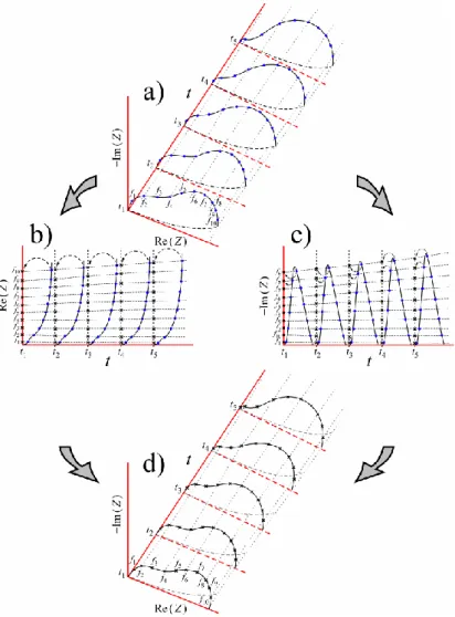
The four-dimensional analysis method is based on the assumption for the continuum of the object’s state and parameters space. (It should be stressed here, that no assumptions concerning the quality or structure of the system under investigation are needed for the application of the method.) It requires several impedance spectra recorded subsequently at the same set of frequencies (Fig.1). Every measured data at a given frequency should additionally contain the time of measurement (these so-called “timestamps” can be the starting or ending times of the measurements of the individual impedance values, arithmetic or other suitably selected averages, etc.). Thus, the experimental data form a set of 4-dimensional arrays, containing frequency, real and imaginary components of the impedance and the time of measurement.
The post-experimental analytical procedure previews the reconstruction of calculated instantaneous impedances. For every measured frequency two one dimensional functions of
4
“iso-frequency dependencies” (e.g. for the real and for the imaginary components) are constructed. Then, each iso-frequency dependence is modeled by an approximating formal model. On the basis of the continuity of the evolution, interpolation (and extrapolation) is performed (e.g. by using interpolating or smoothing cubic spline or other interpolation techniques) resulting in instantaneous projections of the full impedance-time space and
“reconstructed” instantaneous impedances related to a selected instant of the time (i.e. the beginning of each frequency scan) (Fig.1). Thus, a set of impedance diagrams is obtained, containing instantaneous impedances, virtually measured simultaneously. Each of these diagrams can be regarded as a stationary one, free of non-steady-state errors.
Figure 1. Scheme of the mathematical procedure. a) 3-D representation of the impedance and time evolution in Re(Z), –Im(Z) and t coordinates. Re(Z): real part of the complex impedance, Im(Z):
imaginary part of the complex impedance, t: time,. : measured data points (impedances) corresponding to the frequencies fi, ti: starting time of the i-th frequency scan. b) Iso-frequency dependencies and calculation of the instantaneous (corrected) Re(Z) values () by interpolation of
5
the measured Re(Z) data. b) Iso-frequency dependencies and calculation of the instantaneous (corrected) –Im(Z) values by interpolation of the measured Im(Z) data. d) 3-D representation of the
“reconstructed” instantaneous impedances related to the beginning of each frequency scan. :
corrected data points (impedances) corresponding to the frequencies fi
Based on the above, one may conclude that the four-dimensional analysis method is most effective in the correction of low-frequency impedance data. In general, this conclusion is correct. Nevertheless, it has been shown recently that the 4-dimensional analysis method can serve as an efficient tool for the study of non-stationary systems in the higher frequency ranges as well (Ujvári et al 2017, Zalka et al 2017). For instance, the method was successfully applied for the determination of the charge transfer resistance and some other characteristic impedance parameters of the gold
|
poly(3,4-ethylenedioxytiophene) (PEDOT)|
sulfuric acid (aq) electrode corresponding to different time instants, including the time instant just after the overoxidation of the polymer film, i.e. the 4-dimensional analysis method can not only be used for the correction of the existing (experimentally measured) impedance data, but it opens up the possibility of the estimation of the impedance spectra outside the time interval of the impedance measurements. According to the results presented in (Ujvári et al 2017, Zalka et al 2017) the low frequency capacitance (the “redox capacitance” of the polymer film) is almost time independent, the changes of the impedance spectra with time are solely due to time evolution of the charge transfer resistance and the double layer capacitance at the gold substrate/polymer interface. Consequently, the high and medium frequency regions of the impedance spectra are stronger affected by the time evolution than the values measured at low frequencies.These results may also be relevant for bioimpedance technology.
Acknowledgements: Support from the Hungarian Scientific Research Fund, the National Research, Development and Innovation Office – NKFI-OTKA and the European Union (grants No. K 109036 and VEKOP-232-16-2017-00013, cofinanced by the European Regional Development Fund) is gratefully acknowledged.
References
Breugelmans T, Lataire J, Muselle T, Tourwé E, Pintelon R, Hubin A 2012 Odd random
6
phase multisine electrochemical impedance spectroscopy to quantify a non-stationary behaviour: Theory and validation by calculating an instantaneous impedance value Electrochim. Acta 76 375–82
Darowicki K 2000 Theoretical description of the measuring method of instantaneous impedance spectra J. Electroanal. Chem. 486 101–5
Hsieh G, Ford S J, Mason T O, Pederson L R 1996 Experimental limitations in impedance spectroscopy: Part I — simulation of reference electrode artifacts in three-point measurements Solid State Ion. 91 191-201
Hsieh G, Mason T O, Garboczi E J, Pederson L R 1997 Experimental limitations in
impedance spectroscopy: Part III. Effect of reference electrode geometry/position Solid State Ion. 96 153–72
Battistel A, Fan M, Stojadinov J, La Mantia F 2014 Analysis and mitigation of the artefacts in electrochemical impedance spectroscopy due to three-electrode geometry Electrochim.
Acta 135 133–38
Inzelt G, Láng G G 2010 Electrochemical Impedance Spectroscopy (EIS) for Polymer Characterization in Electropolymerization: Concepts, Materials and Applications (Eds:
Cosnier S, Karyakin A) pp 51–76, Wiley-VCH, Weinheim
Keddam M, Rakotomavo C, Takenouti H 1984 Impedance of a porous electrode with an axial gradient of concentration J. Appl. Electrochem. 14 437–48
Láng G, Kocsis L, Inzelt G 1993 Application of the Kramers-Kronig transformation for the data validation of impedance spectra of electroactive polymer films on electrodes Electrochim. Acta 38 1047–9
Lasia A 2014 Electrochemical Impedance Spectroscopy and its Applications, Springer, New York
Louarroudi E, Sanchez B 2017 On the correct use of stepped-sine excitations for the measurement of time-varying bioimpedance Physiol. Meas. 38 N73–80
Savova-Stoynov B, Stoynov Z B 1992 Four-dimensional estimation of the instantaneous impedance Electrochim. Acta 37 2353–5
Stoynov Z 1993 Nonstationary impedance spectroscopy Electrochim. Acta 38 1919–22 Stoynov Z B 1992 Rotating fourier transform-new mathematical basis for non-stationary
impedance analysis Electrochim. Acta 37 2357–9
Stoynov Z B, Savova-Stoynov B S 1985 Impedance study of non-stationary systems: four- dimensional analysis J. Electroanal. Chem. 183 133–44
Stoynov Z, Savova B 1980 Instrumental error in impedance measurements of non-steady-state
7 systems J. Electroanal. Chem. 112 157–61
Ujvári M, Zalka D, Vesztergom S, Eliseeva S, Kondratiev V, Láng G G 2017 Electrochemical impedance measurements in non-stationary systems – application of the 4-dimensional analysis method for the impedance analysis of overoxidized poly(3,4-
ethylenedioxythiophene)-modified electrodes Bulg. Chem. Commun. 49 106–13
Zalka D, Kovács N, Szekeres K, Ujvári M, Vesztergom S, Eliseeva S, Kondratiev V, Láng G G 2017 Determination of the charge transfer resistance of poly(3,4-
ethylenedioxythiophene)-modified electrodes immediately after overoxidation Electrochim. Acta 247 321–32