Cite this article as: Fényes, D., Németh, B., Gáspár, P. (2021) "Stability Analysis of Semi-active Suspension Systems Using a Data-driven Approach", Periodica Polytechnica Transportation Engineering, https://doi.org/10.3311/PPtr.18597
Stability Analysis of Semi-active Suspension Systems Using a Data-driven Approach
Dániel Fényes1*, Balázs Németh2, Péter Gáspár2
1 Department of Control for Transportation and Vehicle Systems, Faculty of Transportation Engineering and Vehicle Engineering, Budapest University of Technology and Economics, H-1111 Budapest, Műegyetem rkp. 3., Hungary
2 Systems and Control Laboratory, Institute for Computer Science and Control (SZTAKI), Eötvös Loránd Research Network (ELKH), H-1111 Budapest, Kende u. 13-17., Hungary
* Corresponding author, e-mail: daniel.fenyes@sztaki.hu
Received: 18 May 2021, Accepted: 15 June 2021, Published online: 06 August 2021
Abstract
The modern vehicles are getting equipped with more and more sensors, which allows the engineers to collect more information about the states of the vehicle and its environment during its operation. This information can be used to increase the capacity and the performances of the control systems. In this paper, a novel data-driven approach is presented to compute the reachability sets of the vehicles, which are equipped with a semi-active suspension system. The dataset, which is used in this paper, is provided by the high fidelity vehicle simulation software, CarSim. Firstly, the dataset is categorized using a stability criterion. Then, a machine- learning algorithm (C4.5 decision tree) is trained, which can categorize a given instance using only the onboard signals of the vehicle.
Finally, a possible application of the reachability sets is presented to show the use of the computed sets.
Keywords
semi-active suspension, data-driven analysis, autonomous vehicles
1 Introduction and motivation
In recent years, the development of fully autonomous vehi- cles has become the main challenge of the automotive industry. This task involves several problems, which must be solved before launching the first self-driven vehicle e.g.
communication (V2X), decision making, and other control problems. In general, the control systems of autonomous vehicles have to deal with three types of motion: longitu- dinal, lateral, and vertical. The longitudinal dynamics of the vehicle can be controlled through the engine and the braking system. The lateral motion of the vehicle can be influenced by the steering system. Whilst, the vertical motion of the vehicle is mainly characterized by its suspen- sion system. There are three different suspension systems:
• Regular, which has no actuator, therefore its dynamics cannot be changed during the operation of the vehicle.
• Semi-active suspension, which has the capability of changing its damping coefficient while driving the car.
• Active suspension, which is equipped with an actu- ator that can be used to realize an additional vertical force. By this additional force, the whole dynamic response of the suspension can be modified.
Obviously, the active suspension is the most benefi- cial from the engineering perspective. However, this sus- pension is more costly than the semi-active one. The gap between the capabilities of the suspensions can be reduced by an intelligent control system. Hence, in the last decades, numerous control strategies and systems have been devel- oped for semi-active suspensions.
One of the most widespread methods for controlling semi-active suspensions is the skyhook control strat- egy (Liu et al., 2019; Shimoya and Katsuyama, 2019).
The basic concept of this strategy is to link the chassis of the vehicle to the sky while simultaneously reducing the vertical acceleration of the vehicle and the axles. Another possibility is the Model Predictive Control (MPC) approach (Rathai et al., 2019a; Rathai et al., 2019b). MPC methods can provide good performances, however, the robustness of these algorithms may be questionable. The robustness of the closed-loop system can be guaranteed by using H∞-based approaches, see (Yu, et al., 2019). However, its performances, sometimes, limited due to their fixed structure. Besides the presented classical (model-based)
approaches, there are other methods, which can deal with this control problem: machine learning-based, data-driven solutions. The machine learning-based approaches have gained wide attention in the last few years. These methods can be a powerful tool for automotive control problems.
For example, a machine learning-based control solution can be found in (Fenyes et al., 2020) for controlling the lat- eral dynamics of the vehicle. An improved MPC algorithm is described in (Fenyes et al., 2019), whose performances are enhanced by a machine learning algorithm.The goal of the paper is to present a data-driven stability analysis for semi-active suspension systems, which can be used as a basis for future control design. The main steps of the algo- rithm are illustrated in Fig. 1.
As it can be seen, the first step is the data acquisition, which is presented in Section 2 The labeling of the dataset is also presented in that section, whose goal is to catego- rize the measured instances according to their stability.
In Section 3 a brief introduction is given to the applied decision tree algorithm, which is used to determine the category of a given instance during the operation of the vehicle. In Section 4 the results of the decision tree are illustrated through different examples. Then, a possi- ble application of the presented reachability sets are pre- sented, which can be found in Section 5 Finally, the contri- bution of the paper is summarized in Section 6.
2 Data-driven stability analysis 2.1 Data acquisition
Since each and every machine learning algorithm requires a lot of data to create appropriate and reliable models, the first step is data acquisition. In this paper, the dataset is provided by the high-fidelity vehicle dynamics simula- tion software, CarSim. In the simulation software, several scenarios have been performed in order to cover a wide range of the operation of the vehicle. During the simula- tions, several parameters of the vehicle and its environ- ment have been changed, such as:
• Longitudinal velocity of the vehicle vx∈{30 90 km/h,− }
• Adhesion coefficient μ∈{0 4 1. − },
• Damping coefficient bx∈{1000 5000 Ns/m,− } (independently on both sides)
• Path of the vehicle (Michigan Waterford hill track, Melbourne Formula 1 track)
During the simulations, the following signals have been measured and collected:
• Longitudinal velocity (vx),
• Steering angle (δ ),
• Angular velocities (yaw-rate ψ, roll-rate ϕ, pitch-rate ω),
• Accelerations (ax, ay, az ),
• Lateral acceleration (ay ),
• Vertical acceleration (az ),
• Side-slip angle of the vehicle ( β ),
• Side-slip angles of the axles (α1, α2),
• Damping coefficients of the suspensions (b1, b2).
In this way, more than 10 million distinct instances have been collected.
2.2 Labeling of the acquired data
Since the main goal of the stability analysis is to separate the stable and the unstable instances from the dataset, a separation criterion must be found. In this paper, a stability criterion will be used, which is based on the two wheeled bicycle model (Rajamani, 2005).The basic idea behind this criterion is to quantify the difference between the lin- ear vehicle model and the measurements. This difference reflects on the nonlinear behavior of the vehicle, which means this difference becomes large when the vehicle enters the highly nonlinear region of its operating range.
< +
+ − − 1 − ≤ 1
l 1 v1x
, (1)
where α1 is the averaged side-slip angle of the front wheels, δ is the steering angle, β denotes the side-slip angle of the vehicle, l1 is the distance between the CoG and the front axle, ψ represents the yaw-rate angle, vx is the longitudinal velocity of the car. Finally, is an experimentally defined parameter.
This inequality is used to divide the dataset into two subsets: acceptable (stable) Racc and unacceptable (unsta- ble) Runa.
3 C4.5 Decision tree algorithm
The presented separation criterion requires the measure- ments of signals ( β, α1, α2 ), which is expensive or cannot be done accurately. Therefore, a machine learning algorithm, more specifically, a decision tree algorithm is used to
Fig. 1 Steps of the analysis process and the application of its results
̇ ̇
̇
β δ
α1 ψ̇
̇
determine the stability of an instance during the operation of the vehicle using only those signals, which are available from the onboard system (accelerations, angular velocities, longitudinal velocity). In the following, a brief introduction is given to the applied decision tree algorithm.
As a first step, the algorithm divides the dataset into two subsets:
• Training set, which is used to produce the decision tree;
• Test set, which is used to validate the resulted tree.
Both subsets consist of instances, which are built up by k attributes (A = A1, A2, ... , Ak ). An attribute represents a specific measurement (signal) or class (stable or unsta- ble instance). A class attribute has predefined discrete val- ues: C = C1, C2, ... , Cn. Note that in this case, there is only one class attribute (the stability), which only has two out- comes: acceptable (stable) Racc and unacceptable (unsta- ble) Runa. The main goal of the algorithm is to find a func- tion, which can accurately map (classify) the instances by the selected class:
DOM A
( )
1 ×DOM A( )
2 ×…×DOM A( )
k →DOM C( )
. (2) The resulted function is ordered into a tree structure, as shown in Fig. 2. A tree consists of nodes and leaves. A node contains a condition (whether the value of an attri- bute is greater or smaller than a given value). A node has two outcomes (depending on the condition). The outcomes can lead to another node or to a leaf. The leaves contain the approximated class of an instance. A more detailed description can be found in (Witten and Frank, 2005).In this paper, the presented decision tree algorithm is used to determine the stability of an instance during the operation of the vehicle with regards to the damping coef- ficient of the semi-active suspension.
4 Example: illustration of the stable regions
In this section, an illustration of the resulted stability sets of the semi-active suspension system is presented. As men- tioned in Section 2, the dataset is provided by the CarSim simulation software. In the simulations, a passenger car
has been used, whose mass was set to m = 1530 kg. The damping coefficients of the left and right suspensions have been modified between bx ={500−4500 Ns/m.}
After the data acquisition and labeling of the data, the machine learning software WEKA is applied to produce the decision tree.
In the following, the stable regions of the semi-ac- tive suspension system are presented using the produced decision tree. The dataset has been divided into subsets using the damping coefficients (bl, br ) and equidistant resolution Δb = 1500 Nm/s. For each subset, a decision tree has been produced. Each tree has high performance, which means their percentage of the correctly classified instances is above 90 %.
In the first case, the longitudinal velocity of the vehi- cle is set to vx = 30 km/h, while the damping coefficients of the suspensions are changed simultaneously between 500–4500 Ns/m. The stable regions of this case are illustrated in the plane of ψ and β in Fig. 3. As the fig- ure demonstrates, the stable sets shrink along with the increasing damping coefficient. It means that the perfor- mance of the vehicles decreases at increased damping coefficients.
In the next case, the longitudinal velocity of the vehicle is set to vx = 60 km/h shown in Fig. 4. The same tendency can be observed as in the previous case. However, the sizes of the sets are smaller at all damping coefficients. This phenomenon can be explained by the increased velocity, which also degrades the stability of the vehicle.
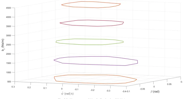
In the next cases, the left damping coefficients are fixed at bl = 500 Ns/m, while the right ones are changed between
br =∈{500−4500 Ns/m.}
Fig. 5 shows the cases when the longitudinal velocity is set to vx = 30 km/h. The same tendency can be observed as in Fig. 5. However, the sizes of the sets become much smaller along with the increasing right damping coefficient.
In case of Fig. 6, the longitudinal velocity of the vehi- cle is fixed at vx = 60 km/h. This figure shows similar ten- dency as presented in the previous cases.
5 Application example and future plans
In this section, a possible application example of the pre- sented reachability sets is presented. The presented sets can be used in the control design of the semi-active sus- pension system. In general, the goal of the control design is to find the balance between the stability of the vehicle and the comfort requirements. It means that the control system must minimize the vertical acceleration:
Fig. 2 Example of decision tree
̇
z1= az →min!, (3) and, in parallel, the displacement of the suspension:
z2 = xv−xs →min!, (4)
where xv denotes the vertical position of the vehicle body and xs is the vertical position of the suspension.
However, both minimization tasks cannot be satisfied at once. Therefore, the primary goal is to ensure the stabil- ity of the vehicle, then to stratify the comfort requirement.
The presented decision trees can be used to compute the bounds of damping coefficients, within which the stability of the vehicle can be guaranteed. It means that the bounds can be computed as:
Fig. 3 Stable sets at vx = 30 km/h
Fig. 4 Stable sets at vx = 60 km/h
bx u T m m
i i n
, =max
( (
1,...,) )
, (5)bx l T m m
i i n
, =min
( (
1,...,) )
, (6)where Ti denotes the produced trees, m1, ... , mn are the measurements from the onboard sensors, bx,u is the upper bound, while bx,l is the lower bound of the damping coef- ficients
(
x∈{ }
r l,)
.For example, these bounds can be used in a Model Predictive Control (MPC) formulation, which can be used to control semi-active suspension system, see in Rathai et al. (2019a). The whole control structure is illustrated in Fig. 7.
The authors' future plan includes the implementa- tion of the proposed control strategy and its validation in MATLAB/CarSim environment.
Fig. 5 Stable sets at vx = 30 km/h, fixed at bl = 500 Ns/m
Fig. 6 Stable sets at vx =60 km/h, fixed bl = 500 Ns/m
References
Fényes, D., Németh, B., Gáspár, P. (2020) "LPV based data-driven modeling and control design for autonomous vehicles", In: 2020 European Control Conference (ECC), Saint Petersburg, Russia, pp. 1371–1376.
https://doi.org/10.23919/ECC51009.2020.9143618
Fényes, D., Németh, B., Gáspár, P. (2019) "Impact of big data on the design of MPC control for autonomous vehicles", In: 2019 18th European Control Conference (ECC), Naples, Italy, pp. 4154–4159.
https://doi.org/10.23919/ECC.2019.8795804
Liu, C., Chen, L., Yang, X., Zhang, X., Yang, Y. (2019) "General theory of skyhook control and its application to semi-active suspension control strategy design", IEEE Access, 7, pp. 101552–101560.
https://doi.org/10.1109/ACCESS.2019.2930567
Rajamani, R. (2005) "Vehicle Dynamics and Control", Springer Science + Business Media, New York, NY, USA.
Rathai, K. M. M., Sename, O., Alamir, M. (2019a) "Reachability based Model Predictive Control for Semi-active Suspension System", In: Fifth Indian Control Conference (ICC), New Delhi, India, pp. 68–73.
https://doi.org/10.1109/INDIANCC.2019.8715601
Rathai, K. M. M., Alamir, M., Sename, O. (2019b) "Experimental imple- mentation of model predictive control scheme for control of semi-ac- tive suspension system", IFAC-PapersOnLine, 52(5), pp. 261–266.
https://doi.org/10.1016/j.ifacol.2019.09.042
Shimoya, N., Katsuyama, E. (2019) "A Study of Vehicle Ride Comfort using Triple Skyhook Control for Semi-active Suspension System", Transactions of Society of Automotive Engineers of Japan, 50(6), pp. 1631–1636.
https://doi.org/10.11351/jsaeronbun.50.1631
Witten, I. H., Frank, E. (2005) "Data mining: practical machine learning tools and techniques", Morgan Kaufmann Publishers, San Francisco, CA, USA.
Yu, S., Zhang, J., Xu, F., Chen, H. (2019) "H∞ Control of Semi-Active MR Damper Suspensions", In: 12th Asian Control Conference, Kitakyushu, Japan, pp. 337–342.
6 Conclusion
In this paper, a data-driven stability set analysis has been presented for semi-active suspension systems. The first step of the algorithm was the data acquisition, which was performed by using the high-fidelity vehicle dynamics simulation software, CarSim. The labeled dataset has been used to produce a decision tree, which was able to categorize the current measurements using only the onboard signals.
Finally, a possible application of the presented decision trees has been shown, in which the decision trees were used to compute the bounds of the damping coefficients.
Acknowledgement
The research was supported by the National Research, Development and Innovation Office through the project
"Integration of velocity and suspension control to enhance automated driving comfort in road vehicles" (NKFIH 2018-2.1.13-TET-FR).
The research was supported by the Ministry of Innovation and Technology NRDI Office within the framework of the Autonomous Systems National Laboratory Program.
The work of D. Fényes was supported by the ÚNKP- 20-3 New National Excellence Program of the Ministry for Innovation and Technology from the source of the National Research, Development and Innovation Fund.
The work of B. Németh was partially supported by the János Bolyai Research Scholarship of the Hungarian Academy of Sciences and the ÚNKP-20-5 New National Excellence Program of the Ministry for Innovation and Technology from the source of the National Research, Development and Innovation Fund.
Fig. 7 Structure of the control system