CFD-based investigation of friction factor in rough pipes with Bingham plastic fluid
Minkó, Martin
1̶ Csizmadia, Péter ̶ Till, Sára
Budapest University of Technology and Economics, Faculty of Mechanical Engineering, Department of Hydrodynamic Systems
H-1111, Budapest, Műegyetem rkp. 3., www.hds.bme.hu
1corresponding author: martin.minko@edu.bme.hu
Received: 3 June, 2021 Accepted:
ABSTRACT
Non-Newtonian fluids are frequently used in mechanical engineering practice, so it is essential to understand their flow behaviour. In this paper, Bingham plastic fluid flow was examined in a straight pipe using numerical flow simulation. In addition, to evaluate the accuracy of the CFD model, the calculated pressure drop values were compared with the Colebrook-White, the Swamee-Jain and the Haaland formulas, and their applicability to the Bingham plastic fluid was also demonstrated. The investigation was performed by hydraulically smooth pipe and four different roughness values of the pipe.
INTRODUCTION
The significant part of the losses in fluid flow systems is the friction loss, which can be highly different for non-Newtonian, Bingham plastic materials than the conventional Newtonian fluids.
Accurate hydraulic sizing is required for energy-efficient operation. Computer simulations have an emerging role in today's engineering, instead of costly measurements and analytical calculations, which cannot be used in more complex cases. The numerical simulations save time and effort for the users, but their use requires validation and circumspect procedure. Computational Fluid Dynamics (CFD) software was used with non-Newtonian Bingham plastic fluid in this paper.
There are many common liquids, which can be described with Bingham plastic characteristics, such as molten chocolate (Chhabra, J.F., Richardson, R.P. (2008)), activated sludge (Seyssiecq, I., Ferrasse, J.-H. and Roche, N. (2003)), tomato paste (Abu-Jdayil, B. et al. (2004)) and toothpaste (Chhabra, J.F., Richardson, R.P. (2008)). The following equation defines the rheological behaviour for these fluids:
𝜏 [𝑃𝑎] = 𝜇𝐵∙ 𝛾̇ + 𝜏0 (1)
where 𝜏 [𝑃𝑎] is the shear stress, 𝜇𝐵 [𝑃𝑎 ∙ 𝑠] is the dynamic viscosity of the fluid, 𝜏0 [𝑃𝑎] is the yield stress of the fluid, and 𝛾 ̇[1/𝑠]is the shear rate. These fluids behave as a rigid body below the specific yield stress but flow as a viscous fluid at higher stresses.
In our study, a type of toothpaste was chosen for the test fluid in the simulations. The yield stress of 𝜏0 = 210 𝑃𝑎, and dynamic viscosity of 𝜇𝐵 = 0.08 𝑃𝑎 · 𝑠, were provided by the manufacturer (Küchenmeister, C., Plog, J.P. (2014)) and were very similar to ones of other kinds of toothpaste (Liu, Z. et al. (2015); Ahuja, A., Potanin, A. (2018)). Figure 1 shows the rheograms of the applied Bingham-plastic fluid compared to the water as reference Newtonian fluid.
The pressure drop along the pipe section was defined by the product of the ζ [-] loss coefficient and the dynamic pressure. For straight pipes, the losses are originated from the friction losses so that the pressure drop can be calculated from the 𝑓 [−]friction factor, the 𝐷 [𝑚] inner diameter and the 𝐿 [𝑚]
length of the investigated pipe section:
∆𝑝′ = ζ ∙𝜌
2∙ 𝑣2 = 𝑓 ∙ 𝐿 𝐷∙𝜌
2∙ 𝑣2 (2),
where 𝜌 [𝑘𝑔/𝑚3] is the fluid density, and 𝑣 [𝑚/𝑠] is the average velocity in the pipe.
The pipe friction factor is the function of the Reynolds number 𝑅𝑒 [−] and the relative pipe roughness 𝜀 [−] of the pipe wall in the case of Newtonian fluids. For laminar flow (𝑅𝑒 < 2300) the 𝑓 = 64/𝑅𝑒 analytical formula is known, and in this laminar region, the roughness of the pipe does not affect the flow (Lajos, T. (2008)). This analytical solution provides that with the modification of the Reynolds number, the friction factor can be calculated with the same equation for non-Newtonian fluids.
Madlener et al. (Madlener, K., Frey, B. and Ciezki, H.K. (2009)) defined the suitable modified Reynolds number 𝑅𝑒𝑚𝑜𝑑 [−] for some types of non-Newtonian fluids. Their formula for Bingham plastic fluids is:
𝑅𝑒𝑚𝑜𝑑 = 𝜌 ∙ 𝑣 ∙ 𝐷 𝜏0
8 ∙ 𝐷
𝑣 + 𝜇𝐵∙3𝑚 + 1 4𝑚
, (3),
𝑚 = 𝜇𝐵∙8𝑣 𝐷 𝜏0+ 𝜇𝐵∙8𝑣
𝐷
(4), where 𝑚 [−] is the local exponential factor.
For turbulent flow in a hydraulically smooth pipe, the 𝑓 = 0.316/∜𝑅𝑒 Blasius-formula is valid up to the Reynolds number of 105 (Lajos, T. (2008)). For power-law fluids, Dodge and Metzner (Dodge, D.W., Metzner, A.B. (1959)) and Tomita (Tomita, Y. (1959)), for Bingham plastic fluids Hanks and Dadia (Hanks, R.W., Dadia, B.H. (1971)) and Swamee and Aggarwal (Swamee, P.K., Aggarwal, N.
(2011)) proposed empirical correlations between the friction factor and the Reynolds number. Turian et al. investigated the friction losses in the laminar, the turbulent and the transition zones with concentrated slurry (Turian, R.M. et al. (1998)).
If we consider a rough pipe wall, there is a large volume of empirical equations for approximate the friction factor with Newtonian fluid, e.g. the Colebrook-White (Colebrook, C.F. (1939)); the Fig. 1. Rheograms of the investigated fluids: toothpaste and water. a) The shear stress as the function of the shear rate. Note that the scales of the two vertical axis are different. b) The apparent viscosity, which is the quotient of the shear stress and the shear rate, as the function of the shear rate.
Swamee-Jain (Swamee, P.K., Jain, A.K. (1976)) and the Haaland (Haaland, S.E. (1983)) equations.
In contrast, only a limited number of non-Newtonian turbulent friction factors exists for rough pipes to date. One of the reasons for this is that the definition of the Reynolds number for non-Newtonian fluids is not yet uniform either; the other is that the validation of the formulas is not obvious.
Our study aimed to investigate the possible applicability of some known friction factor formulas for rough pipes using the modified Reynolds number for Bingham plastic fluids given in Eq.(3). The examined estimations were the implicit Colebrook-White equation:
1
√f = −2 ∙ log10( 𝜀
3.7 ∙ 𝐷+ 2.51
𝑅𝑒𝑚𝑜𝑑_𝐵 ∙ √f) (5),
the explicit Swamee-Jain equation:
𝑓 = 0.25 ∙ [log10( 𝜀
3.7 ∙ 𝐷+ 5.74 𝑅𝑒𝑚𝑜𝑑_𝐵0.9 )]
−2
(6), and the also explicit Haaland equation:
1
√𝑓 = −1.8 ∙ log10(( 𝜀 3.7 ∙ 𝐷)
1.11
+ 6.9
𝑅𝑒𝑚𝑜𝑑_𝐵) (7).
For 4000 < 𝑅𝑒, the limit of the complete turbulence for rough pipes and the appliance of the estimations is (Larock, B.E., Jeppson, R.W. and Watters, G.Z. (1940)):
1
√𝑓 = 1.14 − 2 ∙ log10(𝜀
𝐷) (8).
Beyond this limit, at large Reynolds numbers, the friction factor is independent of fluid viscosity and only depends on the roughness of the pipe (Barker, G. (2018)). This zone was by no means important for the present study, as the lower 𝑅𝑒 values are relevant in engineering applications due to the high viscosity of the tested Bingham plastic fluid.
For Bingham plastic fluids, not only the Reynolds but also the Hedström number (𝐻𝑒) is known as describing a dimensionless group. In our case, the Hedström number was:
𝐻𝑒 =𝐷2𝜌𝜏0
𝜇𝐵2 = 1.09 ∙ 105 (9).
There is known as a criterion for transition from laminar to turbulent flow for Bingham plastic fluid, which can be calculated from the 𝐻𝑒 number (Chhabra, R.P., Richardson, J.F. (1999)). From this, in our case, the critical Reynolds number of 𝑅𝑒_𝑐𝑟𝑖𝑡 = 4670 was specified as the limit of the turbulent flow.
Previous research findings proved that CFD simulations were suitable for modelling the flow of non- Newtonian fluids; e.g. Csizmadia and Hős estimated loss coefficients for Bingham plastic and power- law fluids (Csizmadia, P., Hős, Cs. (2014)), non-Newtonian flow and turbulence models were investigated in anaerobic digesters by Wu (Wu, B. (2011)) and Terashima et al. (Terashima, M. et al.
(2009)). Our CFD simulations were performed with smooth and four different rough pipes in ANSYS CFX® software (Ansys Inc. (2009)) in the range of the modified Reynolds number of 𝑅𝑒 = 0.4 − 40 000.
First of all, the 𝑟𝑝𝑙𝑢𝑔 radius of the plug flow region was verified by comparing the analytical value given for Bingham plastic fluids (Chhabra, J.F., Richardson, R.P. (2008)):
𝑟𝑝𝑙𝑢𝑔 =2𝐿 ∙ 𝜏0
∆𝑝 (10).
For the analysis, a length of 𝐿 = 4𝐷 straight pipe section was selected where the velocity profile is fully developed. The friction factor and the modified Reynolds number were determined with Eq. (2) and Eq. (3) from the pressure drop across this section and the average velocity derived from the CFD simulations. The friction factors were also determined in the laminar region with 𝑓 = 64/𝑅𝑒𝑚𝑜𝑑 ; in the turbulent case (for 4000 < 𝑅𝑒𝑚𝑜𝑑) for smooth pipe with the Blasius equation of 𝑓 = 0.316/√𝑅𝑒4 𝑚𝑜𝑑 and for rough pipe with Eq.-s (5)-(7) as well.
NUMERICAL SIMULATIONS
The geometry for the CFD simulations was a 1/16 longitudinal section of a straight pipe. The actual diameter of the pipe was 𝐷 = 0.05 𝑚; the whole length of the geometry was 𝐿 = 20𝐷 long. The middle of the geometry, near the symmetry axis, has been removed to ensure numerical stability, as shown in Fig. 2.
The meshing procedure and the simulations were carried out in ANSYS CFX®. This software solves the continuity equation, the Reynolds-averaged Navier-Stokes equation (RANS), and the turbulent transport equations (Ansys Inc. (2009)). Furthermore, the material model describing the rheology gives the relationship between the deformation and tension tensors. The built-in k-ω SST turbulence model was used (Barker, G. (2018)). Steady-state simulations were performed. We used the automatic timestep manager and the convergence criteria of root mean square (RMS) for the calculations.
Fig. 2 shows the geometry and the numerical resolution; on the right-hand side, it can be seen that the three-dimensional structured mesh was built containing cube and rectangle elements, and mesh refinement was applied near the friction wall. The grid-independence study was carried out and proved that our mesh of 𝑁 = 105 000 cells was sufficient for our task.
At the upstream boundary, a uniform velocity profile was prescribed. At downstream average static pressure was imposed as a boundary condition. In addition, at the sides of the tube section, symmetry boundary conditions, in the middle by the symmetry axis free-slip wall was applied. Finally, depending on the case, a hydraulically smooth or rough friction wall was defined on the pipe segment.
The specific values of the roughness parameters are summarised in Table 1.
Fig. 2. The geometry and the structured mesh
𝜺 roughness [mm]
𝜺/𝑫 relative roughness [-]
0 smooth
0.05 0.001
0.5 0.01
1 0.02
2.5 0.05
Table 1. The roughness values of the different cases
RESULTS
Validation with water
Test calculations were performed with clean water and a hydraulically smooth pipe wall. The calculated friction factors were compared to the analytical 𝑓 = 64/𝑅𝑒 in the laminar region and the Blasius equation in the turbulent case. In the modified Reynolds number range of 𝑅𝑒 = 100 − 20 000, the differences between the friction factor values were generally less than 5%, except for the laminar-turbulent transition region.
Non-Newtonian fluid
Fig. 3 shows the velocity profile as the function of the dimensionless coordinate in the investigated pipe segment at the average velocity of 𝑣 = 3.4 𝑚/𝑠 with toothpaste. As expected, in the central core, where the shear rate is below the yield stress, a plug flow region, but near the wall, a parabolic profile can be seen. The size of the analytical plug flow region was calculated with Eq. (10) and showed good accordance with the numerical one.
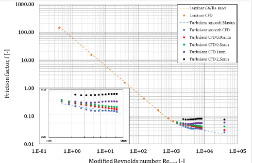
Fig. 4 presents the friction factors from the CFD simulations. In the laminar region, the numerical (orange dots) and analytical (orange dashed line) results showed a good correspondence. However,
Fig. 3. Velocity profile from the CFD results in the pipe at the average velocity of v=3.4 m/s with the analytical plug flow region
in the turbulent case with a hydraulically smooth pipe, the numerical results differed from the Blasius equation, which is plotted in Fig. 4 by the blue dashed line. This discrepancy was present not only in the critical zone but also at higher Reynolds numbers. The average relative difference between the two was 6.5%.
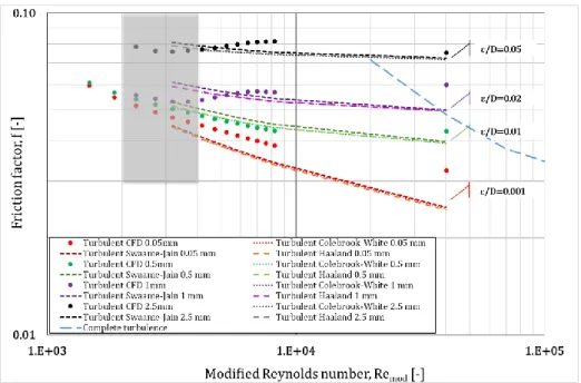
Our results with rough pipes were compared to empirical friction factors as follows the Colebrook- White, the Swamee-Jain and the Haaland formulas given with Eq.-s (5)-(7). As presented in Fig. 5, there were differences of varying degrees between the numerical and empirical results, despite using the modified Reynolds numbers in the empirical equations. The limit of the complete turbulence as in Eq. (8), from where the friction factor is not dependent on the Reynolds number but only on the relative roughness, is also presented. The simulation points with the highest Reynolds numbers at the higher roughness values fell in this range, so they are not relevant to compare with the empirical equations.
Fig. 4. The friction factors derived from the CFD simulations as the function of the modified Reynolds number in all cases: smooth pipe; roughness of 0.05; 0.5; 1 and 2.5 mm.
In addition, orange dotted line shows the f=64/Remod in the laminar region, and blue dotted line shows the Blasius equation for smooth pipe flow
Table 2 compares the relative differences between the different types of estimations at three modified Reynolds number values from the turbulent region. In addition, for the lowest relative roughness of 𝜀/𝐷 = 0.001 the diversion from the Blasius equation is also indicated, which values were in the same magnitude with the others. The results in brackets fell into the range of complete turbulence, so they are not relevant in the comparison.
While at the relative roughness of 𝜀/𝐷 = 0.01 we got a very good match with the maximum difference of 5% between the CFD and the estimations. The difference was also not greater than 10%
in the other relevant cases, except for the lowest roughness. These latter simulation results require further investigation. However, the mean values calculated for the rough, turbulent range for all roughness values, which are given in the last row of Table 2, show no significant difference between the empirical formulas.
Modified Reynolds number 𝑹𝒆𝒎𝒐𝒅 [−]
Relative roughness 𝜺/
𝑫 [−]
Colebrook- White
Swamee- Jain
Haaland Blasius
𝑹𝒆𝒎𝒐𝒅 = 𝟒 𝟏𝟗𝟐 0.001 -10% -8% -9% -12%
0.01 2% 5% 2%
0.02 5% 9% 6%
0.05 -1% 2% 0%
𝑹𝒆𝒎𝒐𝒅 = 𝟖 𝟐𝟎𝟖 0.001 -12% -12% -13% -14%
0.01 2% 5% 2%
0.02 -9% -7% -8%
0.05 -9% -7% -8%
𝑹𝒆𝒎𝒐𝒅 = 𝟒𝟎 𝟐𝟗𝟎 0.001 -24% -23% -25% -31%
Fig. 5. The friction factors from the CFD simulations as the function of the modified Reynolds-number compared to the Colebrook-White Eq. (5); the Swamee-Jain Eq. (6) and the Haaland equations Eq. (7) in the rough cases. The dashed blue line shows the limit of complete
turbulence of Eq. (8), the grey shade shows the critical zone of 2000 < 𝑅𝑒𝑚𝑜𝑑 < 4000.
0.01 -8% -7% -8%
0.02 (-17%) (-16%) (-17%)
0.05 (-5%) (-4%) (-4%)
All Average 8% 9% 8%
Table 2. The relative difference between the friction factors from the CFD simulations and the calculated empirical ones at three specific Reynolds number values
CONCLUSIONS
This study investigated the friction factor in a straight pipe with a non-Newtonian Bingham plastic test fluid (toothpaste) using validated numerical CFD models. The friction factor was determined over a wide modified Reynolds number range and under several roughnesses. Because of using dimensionless numbers, our results can be more widely applicable. Based on the results, the empirical equations available in the literature for Newtonian fluids can be applied in the examined range if the modification of the Reynolds number is described by Madlener et al. (Madlener, K., Frey, B. and Ciezki, H.K. (2009)). Moreover, the average differences between the literature available for Newtonian fluids and CFD calculations are generally less than 10%, but in any case, they remain below 25% in the range studied.
ACKNOWLEDGEMENTS
The work was supported by the New National Excellence Programme No. ÚNKP-20-5-BME-156 of the Ministry of Innovation and Technology Hungary (the award was received by Péter Csizmadia) and by the János Bolyai Research Scholarship of Hungary.
NOMENCLATURE
Notation Denomination Unit
D Pipe inner diameter [m]
𝑓 Friction factor [1]
He Hedström number [1]
L Pipe length [m]
m Local exponential factor [1]
N Number of cells [pcs]
∆𝑝′ Pressure drop [Pa]
rplug Analytical plug flow radius [m]
Re Reynolds number [1]
Remod Modified Reynolds number [1]
v Velocity [m/s]
𝛾̇ Shear rate [1/s]
Absolute roughness heights [mm]
𝜁 Loss coefficient [1]
𝜇𝐵 Dynamic viscosity for Bingham plastic fluids [Pa·s]
𝜌 Density [kg/m3]
𝜏 Shear stress [Pa]
𝜏0 Yield stress [Pa]
Keywords: CFD simulation, rough pipe, fluid flow engineering, non-Newtonian fluid, Bingham- plastic fluid
REFERENCES
Abu-Jdayil, B., Banat, F., Jumah, R., Al-Asheh, S. and Hammad, S. (2004). A comparative study of rheological characteristics of tomato paste and tomato powder solutions. International Journal of Food Properties, 7, 3, pp. 483–497. doi: 10.1081/JFP-200032940.
Ahuja, A., Potanin, A. (2018). Rheological and sensory properties of toothpastes, Rheologica Acta, 57, 6-7, pp. 459–471. doi: 10.1007/s00397-018-1090-z.
Ansys Inc. (2009). ANSYS CFX-solver theory guide, ANSYS CFX Release, vol. 15317, no. April, pp. 724–746. doi: 10.1016/j.ijmultiphaseflow.2011.05.009.
Barker, G. (2018). Chapter 18 - Pipe sizing and pressure drop calculations, pp. 411–472, in: The Engineer's Guide to Plant Layout and Piping Design for the Oil and Gas Industries, Ed. Baker, G., Elsevier Gulf Professional Publishing, Cambridge, USA.
Chhabra, R.P., Richardson, J.F. (1999). Chapter 3 - Flow in pipes and in conduits of non-circular cross-sections, pp. 73–161, in: Non-Newtonian Flow in the Process Industries, Eds.: Chhabra, R.P., Richardson, J.F., Elsevier Butterworth-Heinemann, Oxford, UK.
Chhabra, J.F., Richardson, R.P. (2008). Non-Newtonian Flow and Applied Rheology: Engineering Applications, 2nd ed., Elsevier Butterworth-Heinemann, Oxford, UK.
Colebrook, C.F. (1939). Turbulent flow in pipes, with particular reference to the transition region between the smooth and rough pipe laws, Journal of the Institution of Civil Engineers, 11, 4, pp.
133–156. doi: 10.1680/ijoti.1939.13150.
Csizmadia, P., Hős, Cs. (2014). CFD-based estimation and experiments on the loss coefficient for Bingham and power-law fluids through diffusers and elbows, Computers and Fluids, 99, pp. 116–
123. doi: 10.1016/j.compfluid.2014.04.004.
Dodge, D.W., Metzner, A.B. (1959). Turbulent Flow of Non-Newtonian Systems, AIChE Journal, 5, pp. 189–204.
Haaland, S.E. (1983). Simple and explicit formulas for the friction factor in turbulent pipe flow, Journal of Fluids Engineering, Trans. ASME, 105, 2, pp. 242–243. doi: 10.1115/1.3240975.
Hanks, R.W., Dadia, B.H. (1971). Theoretical analysis of the turbulent flow of non‐newtonian slurries in pipes, AIChE Journal, 17, 3, pp. 554–557. doi: 10.1002/aic.690170314.
Küchenmeister, C., Plog, J.P. (2014). How much squeezing power is required to get the toothpaste out of the tube? Yield stress determination using the HAAKE Viscotester iQ, Thermo Fisher Application Notes, 275.
Lajos, T. (2008). Basics of the flow (in Hungarian). Műegyetem Kiadó, Budapest.
Larock, B.E., Jeppson, R.W. and Watters, G.Z. (1940). Hydraulics of Pipeline Systems, CRC Press, Boca Baton (Florida, USA).
Liu, Z., Liu, L., Zhou, H., Wang, J. and Deng, L. (2015). Toothpaste microstructure and rheological behaviors including aging and partial rejuvenation, Korea-Australia Rheology Journal, 27, 3, pp.
207–212. doi: 10.1007/s13367-015-0021-0.
Madlener, K., Frey, B. and Ciezki, H.K. (2009). Generalized Reynolds number for non-Newtonian fluids, Progress in Propulsion Physics, 1, pp. 237–250. doi: 10.1051/eucass/200901237.
Seyssiecq, I., Ferrasse, J.-H. and Roche, N. (2003). State-of-the-art: Rheological characterisation of wastewater treatment sludge, Biochemical Engineering Journal, 16, 1, pp. 41–56. doi:
10.1016/S1369-703X(03)00021-4.
Swamee, P.K., Jain, A.K. (1976). Explicit Equations for Pipe-Flow Problems, Journal of the Hydraulic Division, ASCE, 102, HY5, Proc. Paper 12146, pp. 657–664.
Swamee, P.K., Aggarwal, N. (2011). Explicit equations for laminar flow of Bingham plastic fluids, Journal of Petroleum Science and Engineering, 76, 3-4, pp. 178–184. doi:
10.1016/j.petrol.2011.01.015.
Terashima, M., Goel, R., Komatsu, K., Yasui, H., Takahashi, H., Li, Y.Y., Noike, T. (2009). CFD simulation of mixing in anaerobic digesters, Bioresource Technology, 100, 7, pp. 2228–2233. doi:
10.1016/j.biortech.2008.07.069.
Tomita, Y. (1959). A study on non-Newtonian flow in pipe lines, Bulletin of JSME, 2, 5, pp. 10–16.
Downloaded 08, August, 2021, https://www.jstage.jst.go.jp/article/jsme1958/2/5/2_5_10/_pdf.
Turian, R.M., Ma, T.-W., Hsu, F.-L. G. and Sung, D.-J. (1998). Flow of concentrated non-Newtonian Slurries 1: friction, losses in laminar, turbulent and transition flow through straight pipe, International Journal of Multiphase Flow, 24, 2, pp. 225–242. doi: 10.1016/S0301- 9322(97)00038-4.
Wu, B. (2011). CFD investigation of turbulence models for mechanical agitation of non-Newtonian fluids in anaerobic digesters, Water Research, 45, 5, pp. 2082–2094. doi:
10.1016/j.watres.2010.12.020.
Circular Economy and Environmental Protection Bilingual scientific journal / Kétnyelvű tudományos folyóirat
KöKörrffoorrggáássooss GGaazzddaassáágg ééss KKöörrnynyeezzeettvvééddeelleemm
Dear corresponding author, Dr. Peter Csizmadia
your manuscript written by Martin Minko, Sara Till and Peter Csizmadia with the title
CFD-based investigation of friction factor in rough pipes with Bingham plastic fluid
is accepted for publication as it stands in Circular Economy and Environmental Protection.
Budapest, 27 August 2021.
Prof. Dr. Peter Mizsey Editor-in-Chief