MAGYAR TUDOMÁNYOS AKADÉMIA
SZÁMÍTÁSTECHNIKAI ÉS AUTOMATIZÁLÁSI KUTATÓ INTÉZETE
A SYSTEM FOR MONITORING THE MACHINING OPERATION IN AUTOMATIC MANUFACTURING SYSTEMS
By
Peter BERTÖK
Tanulmányok 159/1984
A kiadásért felelős DR. VÁMOS TIBOR
Főosztályvezető:
Dv. Nemes László
ISBN 963 311 178 1 ISSN 0324-2951
SZÁ M A LK Repro 84/212
C O N T E N T S
AUTOMATIC Operation of Manufacturing Systems
1.1. Incentives, Aims ... 5
1.2. Automatic Operation of Manufacturing Systems ... 6
1.3. Detection of Failure in Machining ... 10
1.3.1. Functional Overview ... 10
1.3.2. Operation Surveillance Methods ... 13
1.4. Structure of the Present Study ... 16
Measurement of theCutting Torque - Spindle Motor Current Transfer Function 2.1. Introduction ... 18
2.2. The Experimental System ... 19
2.2.1. Configuration of the Experiments ... 19
2.2.2. Data Acquisition System ... 19
2.3. Cutting Torque - Motor Current Transfer Function Measurement ... 22
2.3.1. Transfer Function Calculation Method ... 22
2.3.2. Cutting Experiments ... 23
2.4. Conclusion ... 30
Detection of the Breakage of a Multiple Edged Tool by Autoregressive Modelling 3.1. Introduction ... 31
3.1.1. The Monitoring Methods of this Study ... 31
3.1.2. Tool Breakage and Estimation (Filtering) Theory 32 3.2. The Way of Modelling the Cutting Process ... 33
3.2.1. Estimation ... 33
3.2.2. Stochastic Linear Estimation ... 34
3.2.2.1. Problem Formulation ... 34
3.2.2.2. The Filtering Method ... 34
3.2.2.3. Process Modelling, Autoregressive Model (System Identification) ... 37
3.2.2.4. The Residual ... 39
3.3. Tool Breakage Detection by Autoregressive Modelling .. 39
3.3.1. Breakage Detection Principle ... 39
3.3.2. Experimental Results and Discussions ... 40
3.3.2.1. Experiments and Results ... 41
3.3.2.2. The AR Model for Face Milling ... 46
3.3.2.3. Practical Aspects of AR Modelling ... 48
3.4. Application Experiments ... 57
3.5. Conclusions ... 60
Cutting Torque Estimation System (for Monitoring the Cutting Operation) 4.1. Comprehensive Monitoring (Introduction) ... 63
4.2. Existing Comprehensive Monitoring Systems Based on Current Measurement ... 65
4.3. Basic Features and Functions of the System ... 66
4.4. System Description ... 69
4.4.1. System Architecture ... 69
4.4.2. Geometrical Simulation ... 69
4.4.3. Torque Estimation ... 75
Page
4.5. Validation of the System ... 75
4.5.1. Validation Experiments ... 75
4.5.2. Derivation of the Cutting Torque Equation and its Analysis ... 80
4.6. Applications ... 86
4.6.1. Application Example ... 86
4.6.2. NC Program Verification ... 91
4.6.3. Monitoring the Cutting Process ... 92
4.7. Conclusion ... 92
5. A Microcomputer Based Real Time Monitoring System 5.1. Introduction ... 95
5.2. Structure of the Monitoring System ... 95
5.2.1. Functional Structure ... 95
5.2.2. Data Processing ... 99
5.3. Analytical Monitoring of the Machining Process . 99 5.3.1. Autoregressive Model Construction Using a Fast Calculation Algorithm ... 99
5.3.2. Tool Breakage Detection Algorithm ... 103
5.3.3. Off-Line Toolbreakage Detection Tests ... 107
5.4. Comprehensive Monitoring of the Machining Process 110 5.4.1. Tolerance Calculation ... 110
5.4.2. Monitoring ... 111
5.5. Application Examples ... 114
5.5.2. Analytical Monitoring ... 114
5.5.3. Comprehensive Monitoring ... 117
5.6. Conclusion ... 118
6. CONCLUSION ... 122
ACKNOWLEDGEMENTS ... 128 REFERENCES
5
CHAPTER 1
AUTOMATIC OPERATION OF MANUFACTURING SYSTEMS (INTRODUCTION)
1.1 INCENTIVES, AIMS
As the investment into manufacturing hardware increased, better utilization of equipment became a serious problem. Continuous (three shift) operation not only augments the throughput, but also has the benefit of eliminating warm-up of machines which takes up time otherwise usable for machining. Notwithstanding, due to changing social circumstances it becomes more and more
•v
difficult to have operators in night shifts and week-ends [4]. Untended operation has become a key problem in present manufacturing systems, but existing methods offer only a
limited solution, e.g. [12], [16] , [20] . The main concern is to improve the quality of operation, since the quantitative benefit -the increase in output- is achieved already by the safe operation of additional workshifts. In other words securing workpiece quality and machining safety is more important at present then augmenting the number of products.
6
The rapid technological development of the last decades provided new means for automation of factories too. New electronic devices, familiar in other fields, are moving into the factory; they solve many problems in providing good throughput of manufacturing systems. The new tools do not change the fundamentals of manufacturing, but rather improve the organization and enhance the performance.
Nevertheless, full automation of factories is a very complex task, and although many problems have already been solved, several breakthroughs are necessary before laying down the foundations of this new manufacturing technology. This study is intended to make an investigation into the new ways of manufacturing, especially it deals with the problem of operating the machines without the presence of a human attendant.
1.2 AUTOMATIC OPERATION OF MANUFACTURING SYSTEMS
In a manufacturing system various kinds of tasks have to be performed in order to maintain the continuous operation. The most important of them are:
- to provide the smooth work and tool flow to and from the place of machining
- machining the workpiece
- carrying away the chips removed in machining
- surveillance of the operation, e.g. to measure the finished workpiece, detect abnormal events, etc.
In a conventional manufacturing system an operator performs
all these tasks. The automation of them began in mass production, as the few motions repeated frequently posed an easier problem, and the operation itself was very predictable enabling automated surveillance of the operation. Small and medium size production followed it with considerable delay. Although batch orientation of the latter systems differs from a random like operation, it is still very different from manufacturing in large volumes, and the intelligence of a human operator is necessary in many situations. In the following the small and medium size manufacturing systems are the main subject of consideration.
Today already many of these manufacturing systems operate with a few operators only, nevertheless, full automation in this field has not been achieved yet [5]. The tasks listed previously can be divided into two groups, the first being connected with maintaining the normal operation, and the second with handling abnormal events. They need different approaches, since the tasks have basically different properties. Efficient operation under normal circumstances needs careful planning accompanied by proper preparations. The manufacturing schedule has to be set up, and materials, tools have to be in the right place at the right time. The normal operation is foreseeable and predictable. Abnormal events, on the other hand, come about unexpectedly, neither their occurences nor their consequences can be predicted. When the continuous operation is interrupted by an abnormal event, actions depending on the actual situation have to be taken to
- 7 - CHAPTER 1
8
restore the normal state.
The automation of normal operation is a relatively easier task, since the planning and preparatory work is performed off line; the help of CAD and CAPP (computer aided design and process planning) systems are available for the purpose. For automatic detection and elimination of unexpected events a comprehensive, intelligent system is required. The main task of such a system is to restore the normal operation as soon as possible. This can not always be done real time, some cases, e.g. the repair of a damaged machine tool part, may need a long time. In this case the task is easier, immediate stop of the operation, which prevents the system incurring additional damages, helps in reducing the time spent on repair. In general, the automatic resumption of normal operation can be divided into four phases.
1. Failure detection: This requires continuous or at least continuously repeated check of the operation.
2. Damage assessment: The cause of failure must be localized, the extent of damage must be determined.
No recovery procedure can be initiated before a complete image of the trouble has been obtained.
3. Recovery: All components failed or damaged have to be replaced, and/or their normal state restored in order to be able to continue the operation.
9
4. Resumption of the operation: There are two possible ways to restore the operation
- resumption of the machining at the point where it was interrupted
- beginning to machine a new workpiece, and the previous, not finished one is put aside for further inspection and possible repairs.
To be on the safe side usually the second method is selected even when the workpiece is not damaged irreparably.
The actual state of the system is recognized and analyzed in the first two phases, while steps to continue the operation are taken in the second two phases. Depending on the type of failure detected, different actions have to be taken, no general methods or directions can be formulated.
Looking at a highly automated manufacturing system we can see that smooth workpiece flow is achieved by proper scheduling of the transport system,which uses pallets with automatic changers or robots to load and unload the machines. The CNCs need no operator to load or change part programs, their memory or connection with a central computer can supply the programs necessary to the operation.
Cleaning the machine tools from chips has already been solved by using special conveyor belts and other methods.
Surveillance of the operation is the least automated in manufacturing. It poses more problems, which can be divided CHAPTER 1
into three main groups:
10
- inspection of workpiece quality
- check of proper operation of machinery - supervision of machining.
When checking a workpiece, geometrical accuracy and quality of surfaces are examined. Three-coordinate measuring machines gauge the size of the workpiece, and the quality of surfaces are checked by measuring light reflected from the surface [39] . The check of machinery is usually built into the machines. Early systems had only simpler checks, e.g.
not rotating spindle prohibited feed motion. New, advanced systems have already comprehensive check and give detailed information. Component failure detection is always system dependent, since both failures and actions to be taken when a failure is detected differ from system to system. In the next section methods for detecion of failure in the cutting process is discussed.
1.3 DETECTION OF FAILURE IN MACHINING
1.3.1 FUNCTIONAL OVERVIEW
One of the most pressing problems of manufacturing systems is detection of failures during operation. The necessity of recognition of failures has already been acknowledged more than ten years ago, and different systems have been developed to detect accidents, malfunctions, irregularities in manufacturing systems. Some of the
CHAPTER 1
functions are performed off-line, before or after the machining process. For instance, a common method is checking the tool and the workpiece by mechanical [24]— [25], or optical [38] devices. The size and position of the workpiece can be checked before or after machining as well.
The major setback of these methods is that the check is performed off-line, while the machining process remains without supervision. Abnormal events have to be detected before they cause further damages, and this can be performed only by continuous monitoring of the operation, e.g. [15],
[18]. If a monitoring system is combined with a powerful automatic failure diagnostics and control system, proper actions can be taken to eliminate the problem and the operation can continue after a short break. The continuous operation improves the production utilization of machines and results in higher productivity. At the same time by detecting abnormalities when they occur and not letting them to cause a chain reaction of further damages, higher quality products and reduced scrap are also the benefits of a well designed real time monitoring system.
Initially automation has been applied to mass production systems with large run of identical parts. As this operation is rather predictable, a few relatively simple devices can continuously check it and respond to breakdowns and abnormal events [3]. Small and medium size batch oriented production, on the other hand, handles a wide variety of workpieces, and the continuous check of the
12
operation is a more difficult task. It is fraught with many kinds of unexpected disturbances: the variability of work causes irregularities in stock, uneven tool wear, etc., eventually all being possible sources of failures.
Computer integrated manufacturing, the way of automation in small and medium size manufacturing, can facilitate the monitoring of the operation too. On one hand, data serving later for monitoring purposes can be generated at design or preparation to manufacturing. On the other hand, computers can be directly used for monitoring.
Especially the continuous increase in the performance of computers, combined with steady decrease in prices, makes them attractive for direct application to monitoring. An important question is, how much diagnostics to incorporate in any machine. Adding diagnostic features also increases the number of components in the system and its overall complexity, thereby increasing the chances of a failure, although they are expected to improve the performance of the monitored or checked devices. It is essential to note that diagnostic systems, by themselves, do not improve the reliability of an equipment, and do not increase the mean time between failures (MTBF). But they do facilitate the problem identification and thus reduce the mean time to fix
(MTTF).
In the following an overview of the existing methods is given. The guiding line will be the principle of operation,
1 3
as some methods provide a solution for more problems, and it would be difficult to classify them strictly according to their functions.
1.3.2 OPERATION SURVEILLANCE METHODS
Touch probe methods
One method to examine tool and workpiece is the use of touch sensitive devices [24]— [25]. To check the tool usually a switch is built onto the machine. During check the tool is sent into a predetermined position, where it has to touch this switch. The workpiece can be examined by a touch probe in several points. By using the data of tool location, tool offset data can automatically be adjusted.
The measuring probe supplies data about the location of the workpiece, such as position of holes or planes, and a modification of the actual zero shift can compensate the
inaccuracies.
One of the greatest drawbacks of the method is, that it is off line, the measurement is performed before or after machining. The measurement is also very sensitive to dust;
chips and dirt can hinder the accurate measurement. In spite of the similarity with measuring machines it can not be used for workpiece inspection, the measuring reference must be more accurate than the manufacturing.
CHAPTER 1
14
Nontouch size measuring
Dependence on the accuracy of the manufacturing machine can be eliminated by using an independent measuring device.
One possible solution is using laser interferometry [22].
The measurement is stable in time and there is no need for calibration, it can even measure thermal deformation during machining. A feedback of the measured data to the NC can
significantly increase the accuracy of the next workpieces.
As a laser is a very delicate equipment, it must be well protected against the sprinkling metal chips and coolant being common in every workshop. The measurement is sensitive to dust, not clean surfaces deteriorate the accuracy. Finally it must be noted, that a laser is very expensive.
On line monitoring methods
The monitoring methods are to detect abnormal events during machining. They measure different signals, during machining, and detect abnormalities in them. Some methods use vibration analysis technics [21], [35]. The method has been used to detect excessive wear of drills, as an increase in the vibrations. Similar methods have been used in grinding to detect wear of the grinding wheel. Apparently it works well for single edged tools and continuous cutting, but multipoint tools and intermittent processes -as milling-
15 CHAPTER 1
have not been tested yet.
There are experiments to detect tool wear and prevent tool failure by using heat sensing methods [22], [36], [37].
A heat sensor is placed close to the machining point to measure the radiation during operation. The method,
however, meets with difficulties when coolant is used in machining.
Much attention has been paid to the application of acousto-emission (AE) technics to tool wear and breakage detection [27] — [32]. The sound produced by excessive tool wear, tool breakage, entanglement of continuous chips and possibly by other events can be used to detect these abnormalities. Proper filters suppress the unwanted noises, and the interesting -mainly ultrasonic- sounds inform about the cutting state. The method is said to be able to work in finishing and moderate roughing cuts with a single point tool.
Monitoring the cutting torque or the feed forces is a sensitive method to detect machining troubles, since the torque and the feed forces reflect the cutting state well, but their direct measurement is a complicated task. When the tool is not rotating, as on a lathe, the installation of a measuring device is fairly easy [10] , but the torque measurement on a rotating tool -as in case of milling- needs expensive devices [13]. The output coupling of the analog
16
signal can be performed by using slip rings [33] , which make the data noisy and less reliable, or by employing more expensive signal transmitters [34]. An easier method is to measure the torque indirectly via spindle motor current or the feed forces via feed motor current. This measuring method does not require additional sensors, as currents are usually measured in drive circuits for control purposes.
The transfer function between cutting torque (or feed force) and motor current is linear to such extent that monitoring can be based on this method. The price for easy sensoring is more complicated data processing. The monitoring methods using current measurement are reviewed in section 4.2.
The method of monitoring the cutting process by spindle motor current measurement has been opted in the present study. The main target was to provide reliable monitoring algorithms, while benefiting the cheap and easy sensoring.
1.4 STRUCTURE OF THE PRESENT STUDY
The study concerns on line monitoring of the machining operation. It describes methods to detect troubles and their application to real cutting experiments. The parameter monitored is the cutting torque measured via spindle motor current.
First the validity of the sensoring method is proved by determining the cutting torque - spindle motor current
17
transfer function of the machine tool used. Chapter two describes the experiments performed and the determination of the transfer function.
The next three chapters describe two monitoring methods and their practical implementations. The first method, discussed in chapter three, is a stand alone method, not using auxiliary information. The method is primarily for tool breakage detection. The analyzing method and application experiments are presented.
Chapter four describes a cutting torque estimation system aimed at providing a reference pattern of the cutting torque for comprehensive monitoring. The solution opted also helps in performing the geometrical and technological verification of the NC part program. The structure of the torque calculation system is described together with validation and application experiments.
Next the implementation of the two methods into a 16 bit microcomputer is explained in chapter five. The necessary adjustments are presented with experimental results.
The study is concluded with a summary of the main CHAPTER 1
results achieved
18
CHAPTER 2
MEASUREMENT OF THE CUTTING TORQUE - SPINDLE MOTOR CURRENT TRANSFER FUNCTION
2.1 INTRODUCTION
Monitoring needs a reliable data acquisition from the cutting operation. The parameter monitored is expected to reflect the state of the process well, and the sensors used should be durable and accurate. The cutting torque is a parameter reflecting the cutting state well, but its direct measuring on some machine tools may meet with difficulties.
In case of a milling machine, or a machining centre, the difficulties of measuring in a place where sharp metal chips and coolant fluid sprinkle are combined with the problem of a rotating tool . Measuring the torque indirectly, via spindle motor current, is a more suitable way, as it overcomes these difficulties. In order to prove that sensoring of the cutting torque via spindle motor current is correct, the connection between torque and current has to be determined
19
2.2 THE EXPERIMENTAL SYSTEM
2.2.1 CONFIGURATION OF THE EXPERIMENTS
The cutting experiments were performed on a vertical machining centre (MAZAK V 7.5 with a FANUC System 7 numerical controller) . The tool used in the experiments was a face mill cutter with six throw-away cutting edges. The cutting edges used in the experiments were NX55 type (of the Mitsubishi Kinzoku Corp.). The material of the workpiece was carbon steel, with C = 0.45 %.
2.2.2 DATA ACQUISITION SYSTEM
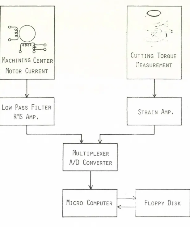
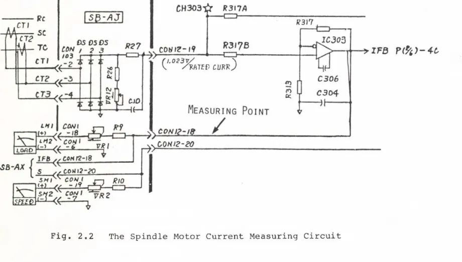
The schematics of the data acqisition is shown in figure 2.1. The spindle motor current was measured in the electronic spindle drive unit.
The cutting torque was measured by strain gauges. The gauges were attached to a specially made workpiece, and the signals were led to a gauge amplifier combined with a low pass filter.
Torque measurement
For torque measurements a special workpiece was made of carbon steel. The workpiece, performing the functions of a dynamometer, comprised of two parts. The lower part, CHAPTER 2
20
Fig. 2.1 Data Acquisition Syst'~
Fig. 2.2 The Spindle Motor Current Measuring Circuit
22
fastened directly on the machine tool table, served as a stand holding the part machined. The two components were fixed together with M14 bolts. The torque was measured on the stand.
Spindle motor current measurement
The spindle motor current was measured in the DC spindle drive unit. The measured current was smoothed by a lowpass filter and a root-mean-square amplifier before the A/D converter sampled the signal.
2.3 CUTTING TORQUE - MOTOR CURRENT TRANSFER FUNCTION MEASUREMENT
2.3.1 TRANSFER FUNCTION CALCULATION METHOD
The input signal 'x(t)' has the spectral density 'Pxx(f)', the output signal 'y(t)' has 'Pyy(f)'. A cross spectral density 'Pxy(f)1 between input and output signals is defined as the Fourier transform of the cross correlation function. The relationship among these functions can be described with the help of the transfer function 'G(f)'.
One relationship describes the connection of the functions a s :
Pxy(f) = G (f) Pxx(f) or
2.1
G (f) Pxy(f) / Pxx(f) 2.2.
23 CHAPTER 2
The coherence function
2 2
ABS [Coh(f)] = ABS [Pxy(f)] /Pxx(f)Pyy(f) 2.3 measures the reliability of the calculations.
2.3.2 CUTTING EXPERIMENTS
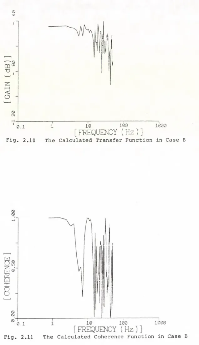
Experiments of two types were performed. As can be seen from figure 2.3, in experiment 'A' a workpiece of round shape was cut vertically. The mean diameter of the workpiece and the diameter of the tool were the same. The workpiece in experiment 'B1, a half cylinder, was cut horizontally. The rim thickness of the workpiece was much less than the diameter of the tool, so the displacement of point of application along the cutting path was negligible.
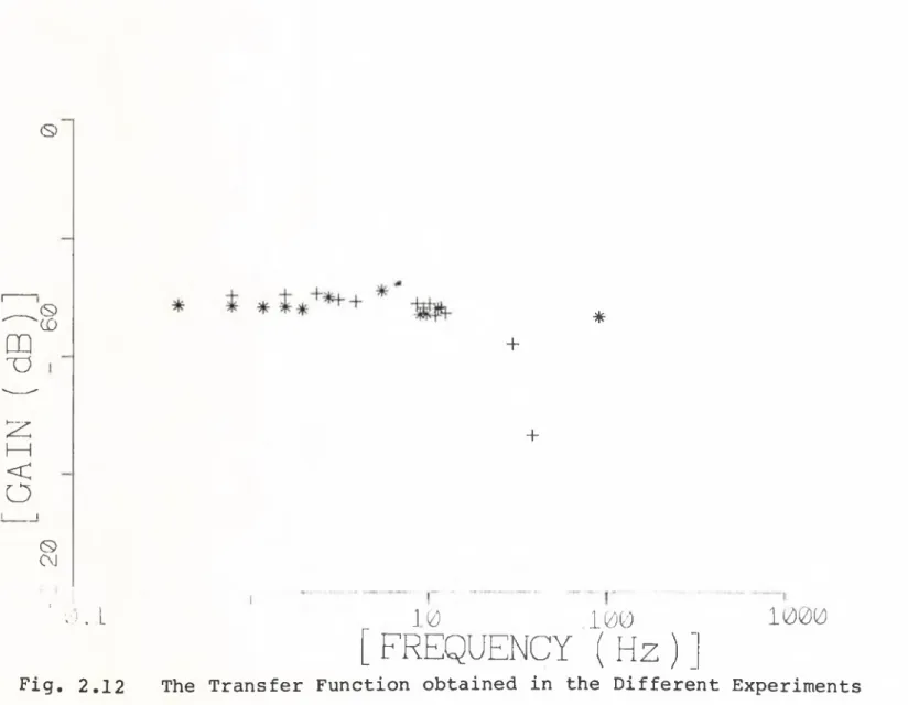
The resultant cutting torque - spindle motor current transfer function obtained by summarizing the results of different experiments is shown in figure 2.12. The figure indicates that the transfer function is constant in the lower frequency range, at least below log omega = 2 , i.e.
below 16 Hz. As the system is supposed to be linear, the break point of the transfer function must be at the highest frequencies of the examined range, or above. As the frequency range examined was that of real cutting experiments, we can conclude that the transfer function of the system is constant in the frequency range used.
24
Fig. 2.3 Cutting Experiments ( A & B Type of Cutting)
CuttingTorque
25
2e
Fig. 2.4 Measured Torque in Cutting Experiment A
<
Fig. 2.5 Measured Current in Cutting Experiment A
[ C O H E R E N C E ] 3 [ G A I N ( d B )1
26
g. 2.6 The Calculated Transfer Function in Case
3s
The Calculated Coherence Function in Cas Fig. 2.7
MotorCurrentCuttingTorque
27
o
Time Fig. 2.9 The Measured Current in .erimént B
[ C O H E R E N C E ] 2 [ G A I N ( d B ) ]
28
©ír
©X)
s:\J
0 1 1 10 100 1000
[ FREQUENCY (Hz)]
g. 2.10 The Calculated Transfer Function in Case B
Fig. 2.11 The Calculated Coherence Function in Case B
; G A I N ( d B )
<S>
r
<S>
CO *
+
I roU3 I +
s>
CM
' A) . 1 ' ] 0 1 0 0 1 0 0 0
[FREQUENCY ( Hz)[
Fig. 2.12 The Transfer Function obtained in the Different Experiments
30
2.4 CONCLUSION
The results indicate that the spindle motor current reflects reliably the cutting torque in the used frequency range. The calculated transfer function was constant in the lower frequency range (about 0 - 1 6 Hz). The spindle motor current is very easy to measure, as spindle drive units measure it for control purposes. On the other hand, as the measuring point is relatively far from the actual cutting point, the information obtained about the cutting process is less accurate. The inertia of the tool and of the spindle gear unit was neglected in the experiments. For a more precise measurement, however, this factor must also be taken into consideration. Finally we can conclude that the cutting state can be reliably monitored via the spindle motor current, as the cutting torque - spindle motor current transfer function can be regarded as constant in the range of cutting signals used.
31
CHAPTER 3
DETECTION OF THE BREAKAGE OF A MULTIPLE EDGED TOOL BY AUTOREGRESSIVE MODELLING
3.1 INTRODUCTION
3.1.1 THE MONITORING METHODS OF THIS STUDY
\
One of the two monitoring methods of this study is presented in this chapter. The two methods use different approaches, as they have different targets. The method described here is to detect tool breakages by detailed analysis of the spindle motor current, and uses no preliminary information about the cutting process in contrast with the comprehensive method described in chapter four. The two methods are complements of each other as far as their applications are concerned, and make up a monitoring system described in chapter five.
Here, after a short section revealing the connection between estimation theory and the examined phenomenon the theoretical background of this method is summarized, then the monitoring method itself and the application experiments
32
are presented. The theoretical summary is based on existing literature. The main points are discussed in respect of the application and special attention is paid to practical problems, such as initialization. The application method is described by relying on the theoretical background. Finally application experiments illustrate the method's performance.
3.1.2 TOOL BREAKAGE AND ESTIMATION (FILTERING) THEORY
In case of single edged tools an efficient solution has been described in [28] for tool brekage detection. Here the case of a tool with more cutting edges is examined.
Our main purpose is the study of small, sometimes microscopic breakages, when the dimensions of the damaged surface on the cutting tip are only within a few millimeters, but we would like to detect greater damages too. Small breakages cause usually small changes in the cutting process, hence their reflection in the cutting torque is also very weak. The mean of the signal does not change significantly, therefore a method monitoring it can detect no abnormality in the signal. The methods comparing the signal with maximum values or with a reference pattern are monitoring the running average of the signal, in order to include some tolerances, so they miss this kind of failures. This type of phenomena are usually examined by using spectrum analytical methods. There are some new methods in spectrum analysis, which offer advantages over
3 3
classical methods in computation and evaluation as well.
These methods are closely related to estimation and filtering theory, in fact they are a special application of it.
CHAPTER 3
Based on linear estimation and filtering theory a method for detection of cutting edge breakage in case of a
tool with more cutting edges is proposed in this chapter.
3.2 THE WAY OF MODELLING THE CUTTING PROCESS
3.2.1 ESTIMATION
The estimation problem consists in determining a model, which approximates to the time history of the system from
the erroneous measurement.
A problem of great importance is determining the parameters of a model based on observations of the physical process being modelled. In some cases the system parameters can not be determined a priori or they vary during system operation. In such case a model can be used, which depends explicitly on these parameters. Based on data from the physical plant and from the model a parameter identifier adjusts the model on-line, thus performing a real time system identification. The method described here follows a similar way. A model describing the physical process is chosen, and its parameters are estimated recursively. The tool breakage is detected as a change in the physical
3 4
process, which is reflected in the system model updated real time.
3.2.2 STOCHASTIC LINEAR ESTIMATION
3.2.2.1 PROBLEM FORMULATION
We consider a dynamic system whose state in time is described by the function 'x(t)'. The discrete case is discussed here only, i.e. when the state of the system is given at (usually equally spaced) time instants. We are interested in knowing the value of 'x(k)' for some fixed 'k', but this 'x(k)' is not directly accessible to us for observation. On the other hand we have a sequence of measurements z(l), z(2), ... z(j), which are causally related to x(k). The estimation problem is to determine a function between 'x' and 'z' in some rational and meaningful manner. If k=j the problem is called filtering, if k>j it is prediction and if k<j it is smoothing or interpolation.
3.2.2.2 THE FILTERING METHOD
The filter we consider has the following equations:
X(n,n-1) = H(n) X(n,n) 3.1
P(n,n-1) = H(n) P(n-l,n-l) H'(n) 3.2 P(n,n)
-1
[P (n,n-l) + M'(n)V -1
(n)M(n) ] -1
3.3 -1
= P(n,n) M'(n) V (n) 3.4
G(n)
X(n,n) = X(n,n-1) + G(n) [z(n) - M(n) X (n,n-l) ] 3.5.
3 5
CHAPTER 3
These equations mean that first, in equation 3.1, the previous estimation is updated according to the state transition equation. Then correction gain 'G' is computed with the help of estimation covariance ' P', observation mechanism 'M' and noise variance ' V in equations 3.2 - 3.4.
Finally equation 3.5 gives the new estimate . Using the so called matrix inversion lemma equations 3.3 - 3.4 can be transformed into a different form, and a new, algebraically equivalent algorithm is resulted in:
X(n,n-1) = H(n) X( n-l,n-l) 3.6
P( n,n-l) = H(n) P(n-l,n-l) H'(n) 3.7 -1 G(n) = P(n,n-1) M '(n)[V(n)+M(n)P(n,n-l)M'(n)] 3.8 P(n,n) = [E - G(n)M(n)] P(n,n-1) 3.9 X(n,n) = X(n,n-1) + G(n) [z(n)-M(n)X(n,n-l)] 3.10
where 'E' is the unit matrix [7], Equations 3.6 - 3.10 represent a simpler form of the Kalman filter, when the plant noise is omitted from the model. The previous form, equations 3.1 - 3.5, is usually titled the sequential estimator, and as it can be derived by using Bayes' theorem on conditional probability sometimes it is also referred to as Bayes-filter. The filters satisfy the minimum variance criterium, in fact they are recursive formulations of it.
As far as computational features are concerned, the two formulas have significant differences. The Kalman formulation requires the inversion of only one matrix, which
36
has the same order as the observation vector. The other formulation calls for the inversion of at least one matrix of the order of the state vector. The simpler calculation can be a deciding factor in some applications.
A problem with the Kalman formulation is the initialization. In the first formulation we can select an initial vector ’X(1,0)' completely arbitrarily, and then by setting the inverse of the covariance matrix singular, i.e.
-1
P (1,0) = 0 3.11
we make the subsequent estimate totally independent of
’X(1,0)'.
In the Kalman formulation, however, this can not be done, since setting
P(1,0) = c E 3.12
('c' means a very great scalar and * E 1 is the unit matrix), and substituting it into 3.8 and 3.10 we will get a result, in which 'X (1,0) 1 will enter into the first estimate.
Therefore in order to start the filtering succesfully, a preliminary information included in the initial vector
'X (1,0)1 is necessary.
Too accurate measurements, i.e. when the variance of the measurement error is very close or equal to zero (V=0), can also cause troubles: the estimation variance matrix
3 7
CHAPTER 3
'P(n,n)' will be singular. Theoretically it is impossible, but due to finite accuracy of our computers a small noise variance can be wiped out completely by computer roundoffs, and the matrix 'P' will be positive definite only marginally and then degenerate into indefinite. This makes the whole process unreliable and the filter be divergent. Thus the Kalman formulation runs into trouble in trying to process too precise observations. In this work larger noise variances were used to circumwent this problem.
3.2.2.3 PROCESS MODELLING, AUTOREGRESSIVE MODEL
In many applications the so called autoregressive moving average (ARMA) models have proven to approximate deterministic and stochastic discrete time processes well.
They are especially popular in human speech analysis, seismic data, ocean wave data analysis and others [8], [10] . Here an attempt is made to apply it to cutting data analysis.
The model expresses the output sequence with the following equation:
(SYSTEM IDENTIFICATION)
P q
I
a'(k) X(n-k) = I b ' (1) u(n-l) 3.13k =0 1 = 0 or
P q
X(n) =-
I
a(k) X(n-k)+I
b (1) u(n-l)k = 1 o -
1
n= 0
3.14 where 'X(n-k)' denotes the outputs and 'u(n-l)' the inputs
3 8
of the system. The coefficients 'a(k)' and 'b (1) * have to be determined by some parameter identification method. The first term on the right side of equation 3.14, which contains only the signal's past is called the self regressive or autoregressive (AR) branch, the second is the moving average (MA) branch of the model. It is very interesting that a general ARMA or an AR process can be represented by a MA model, and an ARMA or MA process can be modelled by an AR one, but in the adequate model the order will be higher, maybe infinite [9]. The AR model, requiring only linear equations for parameter identification, has a computational advantage over the other two.
For sequential estimation of AR parameters the recursive least square method gives a straightforward solution with a fair computational load. The procedure can be interpreted as a Kalman filter. The basic problem is to find the least sqare solution of the AR parameter estimate vector for the observed process. Considering the following system equations:
X (k+1) = X(k) 3.15
z(k) = M(k) X(k) + v(k) 3.16
an estimation can be performed either with equations 3.1 - 3.5 or 3.6 - 3.10.
3 9
CHAPTER 3
3.2.2.4 THE RESIDUAL
The difference of estimated and actually measured data has great importance in estimation technics and usually it is referred to as the residual. It is used in the algorithms to correct the estimation, as we have seen. New observations bring new information about the physical process, and in this way the estimator's knowledge about the process is innovated, therefore it is also termed innovation process [13] , [14] , [15]. The residual will increase when the process changes abruptly, because the model follows the process with a delay, and the change appears in the model only after a time lag. This suggests, that the residual can be monitored to detect abrupt changes in the process.
3.3 TOOL BREAKAGE DETECTION BY AUTOREGRESSIVE MODELLING
3.3.1 BREAKAGE DETECTION PRINCIPLE
A model of the cutting process is built up in the computer, and its output is regularly compared with the physical process. When the physical process changes due to a breakage, the approximation by the original model deteriorates, giving worse results, and the difference between the output of the model and the monitored parameter of the current physical process increases. Accordingly, an unexpected increase in the difference between the model output and the monitored process parameter shows the
4 0
deterioration of the model, which, on the other hand, indicates an unexpected change in the machining process: a tool breakage.
Practical considerations
The first step towards computerized processing of cutting data is to find an adequate model of the cutting process. It is not our aim to find a general comprehensive model as far as cutting dynamics is concerned. On the other hand, the model should be in good correspondence with the real process and give a similar output, in order to be able to use it for monitoring purposes. An AR model is easy to handle in a computer, as the system equations are linear.
And even if the process turns out to have a moving average branch, an AR model of higher order will give satisfactory results. In the following a method for describing the cutting process by an AR model and its application to detect tool breakage caused changes in the signal will be discussed.
3.3.2 EXPERIMENTAL RESULTS AND DISCUSSIONS
For cutting data analysis and tool breakage experiments the milling operation was examined. The face milling process has been chosen for the experiments, since
- in face milling the cutting forces are large, which may cause more frequent breakages
CHAPTER 3
- the use of throw-away tips in face mill cutters and their easy replacement make the experiments easier to perform
Nevertheless, it must be stated that cutting experiments suggest very close similarity between face and end milling.
3.3.2.1 EXPERIMENTS AND RESULTS
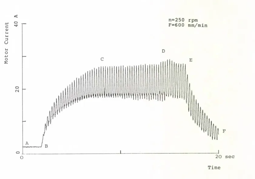
An example of a typical small breakage is shown in figures 3.1 - 3.3. The experiment was performed on a vertical machining centre (Yamazaki V 7 .5). The tool used was a six-tooth face mill cutter, 125 mm in diameter, which cut a workpiece made of carbon steel (C= 0.45 %). The cutting conditions were the following:
cutting speed = 15.625 m/min (250 rpm) feed rate = 0.4 mm/tooth (600 mm/min)
The experiment can be followed in figure 3.1. First the tool was rotating in the air while moving ahead in feed direction, this was the "air cutting". At point 'B' the foremost part of the tool entered the workpiece material, then at 'C the full cutting width was reached. The breakage occured at point 'D1, and at point 'E1 the cutting width began to decrease as the tool went out of the workpiece. The periodicity of the signal corresponds to the spindle speed, the distance in time between two peaks is one revolution. The signal before the breakage is shown in figure 3.2, after enlarging along both axes. The graph reveals, that the tool had some eccentricity, one of the
MotorCurrent
<
Fig. 3.1 Measured Spindle Motor Current (Sampling Interval=5msec)
4 3
n=250 rpm F = 6 00 mm/min
Fig. 3.2 Measured Spindle Motor Current before Tool Breakage
Sampling Interval = 5 msec
n=250 rpm
Time Fig. 3.3 Measured Spindle Motor Current after Tool Breakage
Sampling Interval = 5 msec
44
teeth had a greater share from cutting than the others. The high peaks preceded by falls in the signal suggest, that a tooth had to cut thicker chips than the others. Figure 3.3 shows the signal after the breakage. A smaller peak is present yet at the left side of the graph, but it disappears in the following revolution by rising to the level of the higher peak. This can be explained in that way, that one tooth has broken but continued cutting. Cutting with a broken edge required greater force, which caused a rise in the torque.
The detection signal
The calculated detection signal is shown in figure 3.5.
Figure 3.4 shows again the measured motor current, but here the sampling time was twenty milliseconds. (Only every fourth data of the original set were used.) The change in the current (torque) signal became more difficult to recognize with human eye, but it is still visible. The output of the monitoring system, the residual, was enlarged by twenty times in figure 3.5 in order to make it visible.
Between points 'A1 and 1A l 1 the AR model is adjusting itself to the process and there is no output. After point 1A l ' the output is already valid. The real cutting begins at point 'B'. As the physical process changed, i.e. the tool began to cut the workpiece, there is some difference between the model and the process, and this is reflected in the increase of fluctuations in the residual. After a transient period
Residual
45
<
Sampli:.:: Interval = 20 msec
p=28 V=0.02%
<
sec Time Fig. 3 r 5 Tool B re a k a g e Detection Signal
4 6
the fluctuations decrease, the greater peaks fade away, which shows that the model readjusted itself to the process.
The residual does not show any special mark at point 'C where the tool reached the full width of cut. In point 'D' there is a large spike indicating the tool breakage. As the cutting process changed abruptly, the amplitude of the peaks is about twice as great as in point 'B'. Also, there are large individual peaks rather than a general increase in the amplitude of the fluctuations. The peaks fade away similarly to point 'B1, indicating that the model readjusts itself to the changed process. In point 'E1 the foremost point of the cutter reached the end of the workpiece, and began to leave the workpiece. Comparing the points 'B', 'D' and 'E' we can see that the peaks are the smallest at 'B'.
It is also apparent^ that at 'B' and 'E' the fluctuations increase in the residual, while at 'D' only individual peaks can be observed. From a different point of view we can say that while the changes in the process at points 1 B' and ' E' are fairly slow and can be predicted if the workpiece is known, the change of the process at point 'D' is fast and unpredictable.
3.3.2.2 THE AR MODEL FOR FACE MILLING
The method of AR modelling was that the coefficients of the model, expressing the actual data as a linear combination of the previous data, were recursively estimated by a Kalman filtering algorithm. In other words, the AR
4 7
model says that each time an additional observation of the signal 'z' was attained, it was expressed in the form:
z (k) = M(k) X(k) + v(k) 3.17
where 'M' denotes the vector of prevoius observations, 'X' is the coefficient vector to be determined and 'v* is some unknown disturbance supposed to be a zero mean white noise process independent of the observed signal. The updating of
'M' is a simple shifting operation, the new data steps in and the oldest one is dropped out of the observation vector.
Applying the set of equations to this case we get the following:
P(n) = P(n-1) -
-1
-P(n-1)M'(n)[V+M(n)P(n-1)M1(n)] M(n)P(n-l) 3.18 -1
X(n) = X(n-l)+P(n)M'(n)V (n)[z(n)-M(n)X(n-1)] 3.19 where 'P1 is the estimation covariance and 1V is the noise variance. The noise variance was supposed to be constant.
Using 3.18 and 3.19 the coefficient vector of the AR model, 'X', was recursively estimated. Then by using the coefficients an AR model was built up and the output was calculated at every step. The initial value of every variable was taken as zero, except for the estimation covariance, which was taken as unit matrix.
CHAPTER 3
4 8
3.3.2.3 PRACTICAL ASPECTS OF AR MODELLING
Determination of the model order
Several criteria have been introduced for selection of the AR model order, i.e. to determine how many previous data are needed to estimate the signal reliably [19] - [25].
These criteria give considerable help in selecting a proper order. Nevertheless, when using them against actual data rather than simulated processes, their performance may worsen [26], and in the final analysis subjective judgement can not be eliminated.
The first method discussed is called the final prediction error (FPE). The FPE for an AR process is defined as
2 -1
FPE(p) = s (k) (N+p+1)(N-p-1) 3.20 where s(k) is the average prediction error of the model, 'N'
is the number of data samples and 'p' is the model order.
The FPE increases as 'p* approaches 'N', which reflects the increasing uncertainity of the estimation. The order 'p' selected is the one for which FPE is the least.
Another selection criterion determines the model order by minimizing an information theoretic function introduced by Akaiké. Assuming the process has Gaussian statistics, this information criterion (AIC) is defined as
49
AIC(p) = N ln FPE + 2p 3.21.
Here again the model selected is the one for which the AIC is the least. As 'N' increases, the two criteria, FPE and AIC, will approach each other.
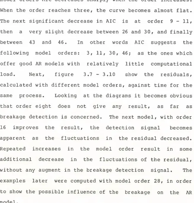
Figure 3.6 shows the AIC against model order for the example shown previously. It can be seen that for very low model orders AIC decreases sharply when the order increases.
When the order reaches three, the curve becomes almost flat.
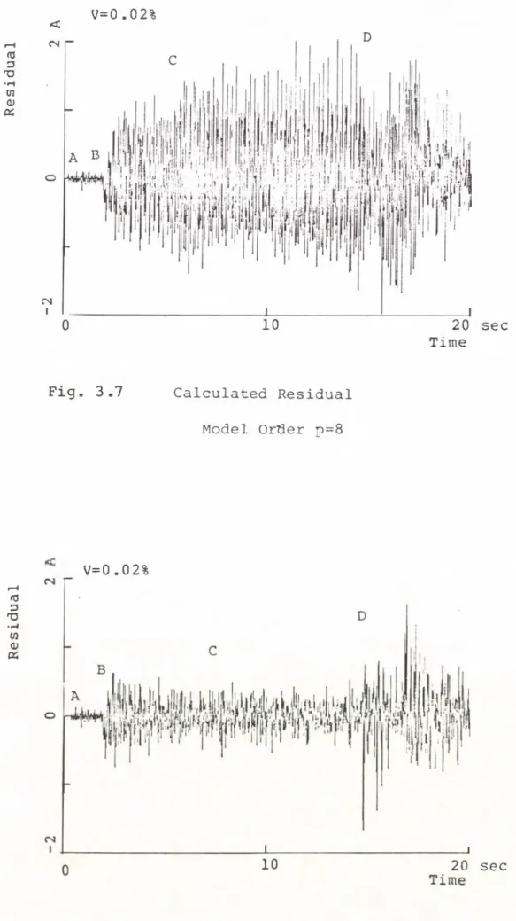
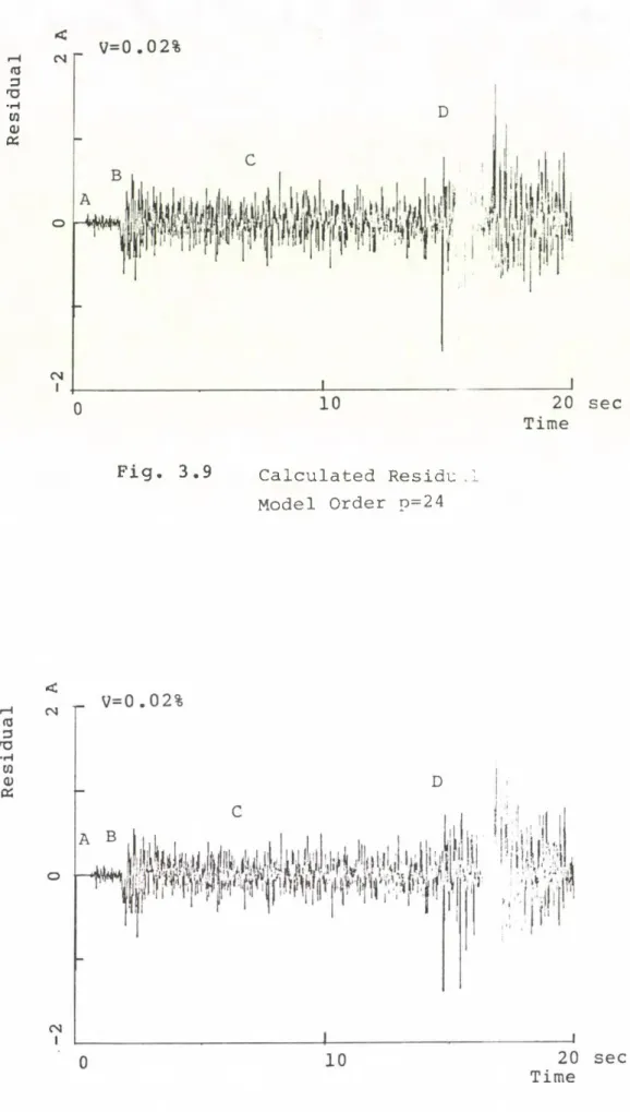
The next significant decrease in AIC is at order 9 - 11, then a very slight decrease between 26 and 30, and finally between 43 and 46. In other words AIC suggests the following model orders: 3, 11, 30, 46; as the ones which offer good AR models with relatively little computational load. Next, figure 3.7 - 3.10 show the residuals, calculated with different model orders, against time for the same process. Looking at the diagrams it becomes obvious that order eight does not give any result, as far as breakage detection is concerned. The next model, with order 16 improves the result, the detection signal becomes apparent as the fluctuations in the residual decreased.
Repeated increases in the model order result in some additional decrease in the fluctuations of the residual, without any augment in the breakage detection signal. The examples later were computed with model order 28, in order to show the possible influence of the breakage on the AR model.
CHAPTER 3
CD
0
Fig. 3.6
PODEL nRDER
Information Criterion by Akaiké
ResidualResidual
51
V=0.02%
<
Fig. 3.7 Calculated Residual Model Order p=8
V=0.02%
sec
sec
Fig. 3.8 Calculated Residual Model Order p=16
Residual
5 2
Fig. 3.9 Calculated Reside.I Model Order p=24
<
Fig. 3.10 Calculated Residual Model Order p=32
5 3
CHAPTER 3
Summarizing the results on model order determination we may conclude that although there are some theoretical criteria, the best and most reliable method is finally a subjective judgement. At least one whole revolution must be included in the data processed (twelve samples were taken from every revolution), and further increase in the order may be useful, as the breakage may cause change in higher coefficients of the model too. The inclusion of two revolutions proved to be sufficient. The detection signal not necessarily improves when the order of the model increases, but the tendency exists, and an optimum must be found.
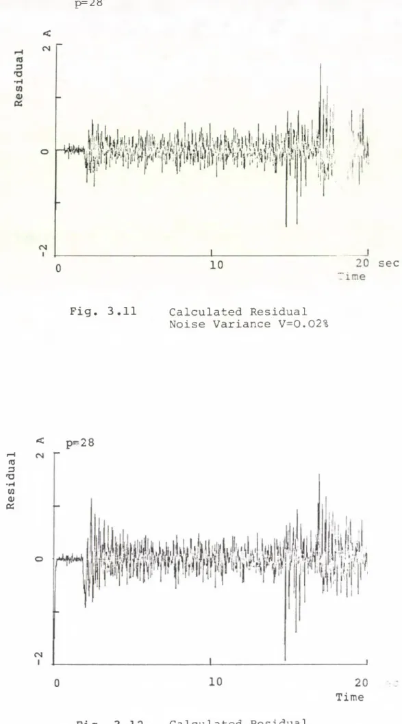
The observation noise variance
Although the supposition of a noise describing the uncertainities and inaccuracies in the measurement system is well founded, there are no good methods to measure any parameter of it. The assumption that it is a zero mean white noise independent of the observed cutting process is plausible and all we need to estimate the model is the noise variance ' V ; it was supposed to be constant in the experiments. Figures 3.11 - 3.12 show the results of different calculations: the residuals calculated with different noise variance against time. The order of the model was 28. The smallest value of the noise variance was about 0.02 % of the signal mean, its absolute value being 0.1. The result shown in figure 3.11 is very good, the
Residual
5 4
p=28
<
Fig. 3.11 Calculated Residual Noise Variance V=0.02%
<
p-28Time
sec
F i g 0 3.12 Calculated Residual Noise Variance V=20%