Research 33(6l6)-6^00;

SHOCK L A Y E R STRUCTURE AND

ENTROPY L A Y E R S IN HYPERSONIC CONICAL FLOWS Robert E. MelnilJ and Richard A. Scheuing^

Grumman Aircraft Engineering, Corp., Bethpage, New York

ABSTRACT

This paper is concerned with the problem of obtaining uni- formly valid solutions to the nonlinear conical flow equations in the thin-shock-layer limit. The basic thin-shock-layer theory is shown to be non-uniformly valid on certain crossflow surfaces. The non-uniformities are of the general type referred to as entropy layers. Uniformly valid solutions are obtained

"by applying the P.L.K, method and G. Carrier's boundary layer technique. The two approaches are shown to lead to similar results.

INTRODUCTION

In this paper the problem is considered of obtaining uniformly valid solutions to the nonlinear conical flow equations in the thin-shock-layer limit. The application of thin-shock-layer theory to conical flows has been considered, and the various approaches (Refs. 1-7) reviewed briefly in order to present an overall view of work accomplished to date in this field.

In his first paper on the subject, Gonor (Ref. l) considered the particular case of hypersonic flow of a perfect gas over a yawed right circular cone. He simplified the equations by in- troducing a variant of the Von Mises streamline coordinates.

Then, assuming analyticity with respect to the density ratio across the shock, he expressed the solution of the transformed equations as a power series in terms of the limiting density

Presented at ARS International Hypersonics Conference, Cam- bridge, Massachusetts, August l 6 - l 8 , 1 9 6 1 . This research has been supported by the Flight Control Lab. of the USAF Aeronauti- cal Systems Division under Contract no. AF 33(6l6)-6^00; the Air Force technical representatives are D. Hoak and H. Max Davis.

Research

^Assistant Chief of Research.

ratio. Only the lowest order equations, which govern the limit- ing flow, were considered further. The solutions to these equa- tions, given in terms of two quadratures, indicate that the crossflow streamlines terminate on the cone surface. Gonor then reasoned that if the body surface is a stream surface in the exact solution, an entropy layer must he present in the approxi- mate solution.

In a later paper (Ref. 2 ) , Gonor extended the previous analy- sis to include arbitrary conical bodies. The generalization was made by using general conical coordinates, taking the body as one of the coordinate surfaces. The equations, similar to those appearing in the rigjat-circular-cone case, are complicated by the presence of the scale factors for the coordinate system.

In practice these scale factors are lengthy and difficult to evaluate for a general body surface. Gonor applied the theory to elliptic cones and flat delta wings at yaw, for both of which the scale factors can be determined explicitly. The calculation for the delta wing was carried out to second order in the den- sity ratio. To this order the shock wave is shown to consist of two planes which intersect in the plane of symmetry. The lateral velocity is nonzero at this point and the solution is singular there. An investigation of the behavior of the solu- tion for the elliptic cones indicates that the singularity does not occur for any small value of the semiaxis ratio greater than zero.

In a general paper on inviscid hypersonic flows (Ref. 3 ) , Scheuing reported on a similar investigation carried out inde- pendently at Grumman. In this investigation Gonor¹ s original work was extended to smooth but otherwise arbitrary conical bodies. The work differed from Gonor1 s treatment (Ref. 2) of the same problem in several respects. Gonor restricted his analysis to perfect gases and chose a coordinate system that required one to calculate a pair of mutually orthogonal conical surfaces for each body shape. It was an almost trivial matter to incorporate equilibrium real gas effects into the analysis as reported in Ref. 3· ^ ^e coordinate problem was considerably simplified by use of a boundary layer type of coordinate system which eliminated the computation of the orthogonal surfaces.

In Ref. 4, Cheng considered the hypersonic flow over a slightly yawed, right circular cone. He expressed the solution as a

triple power series in terms of parameters that are essentially the density ratio, inverse of the Mach number squared and the yaw angle. He was able to solve the resulting equations in the physical plane. The procedure is thus a thin-shock-layer analog of Stone¹ s theory (Ref· 8) . Cheng obtained solutions for the first three terms in closed form and listed them in his report.

He studied third-order effects and encountered the logarithmic singularities in the density, radial velocity and the entropy on the body surface that signal the presence of an entropy layer.

The singularity is shown to be caused by the non-uniformity of the series expansions. On the basis of a reasonable assumption for the functional form of the lateral velocity, Cheng was able to obtain an explicit solution valid within the entropy layer.

Cheng also considered in general terms the behavior of the flow of a real gas in the immediate vicinity of a three-dimensional pointed body. He then considered the implications his analysis had on the study of hypersonic viscous boundary layers and in- dicated the general applicability of a small crossflow analysis for this problem.

Thin-shock-layer theory for right circular cones at small yaw was also developed by Freeman (Ref. 5 ) anä. Guiraud (Ref. 6 ).

Freeman, considering only lowest order effects in the density ratio, extended thin-shock-layer theory to include arbitrary three-dimensional configurations. He specialized the theory to a right circular cone at yaw, treating the yaw effects by a power series expansion in the yaw angle. Explicit results were given for terms up to second order in the yaw angle.

In Ref. 6 Guiraud, using the formal method of asymptotic ex- pansion, gives an elegant derivation of thin-shock-layer theory applicable to arbitrary three-dimensional surfaces. Guiraud carries the process to second order and applies his general theory to a number of specific problems, including the yawed right circular cone. Guiraud, as did Cheng and Freeman, treated the yaw effects by expanding the relevant functions in power series in the yaw angle. The calculations are carried out to second order and the logarithmic singularity present in both Cheng's and Stone's analyses again appears, which is not sur- prising since, for this problem, Cheng's and Guiraud's solution are identical. Guiraud noted the relationship between the log- arithmic singularity and the entropy layer but did not pursue the matter further.

As part of their general studies in Newtonian flow, Hayes and Probstein in their text (Ref. 7) considered the Newtonian flow near the axis of symmetry of an arbitrary conical surface. They were able to obtain particularly simple solutions that clearly illustrate the centrifugal and nonaxially symmetric effects.

Although some of the investigators noted the existence of non- uniformities in the basic approximation, none except Cheng were concerned with the problem of obtaining a solution valid in the entire region of disturbance. However, Cheng's analysis is re- stricted to small deviations from axial symmetry. In the present

analysis it is shown, as was shown by Cheng, that non-uniformi- ties and the associated entropy layers occur in other more gen- eral cases. Therefore there appear to be entropy layer phenom- ena associated wholly with the thin-shock-layer approximation and it is with these non-uniformities that the present investi- gation is concerned. Since the non-uniformities are intimately linked to the topological structure of the crossflow streamline patterns, major emphasis is placed on this facet of the problem.

It should be mentioned that the present authors are not con- cerned with the zero pressure singularity which plagues all of Newtonian theory. This singularity was studied in the axisym- metric and two-dimensional cases by Freeman (Ref. 9)> "wko ob- tained discouraging results respecting practical applications of the theory to flows which exhibit such singularities. In addition the present paper does not consider the Newtonian shock lines discussed in Ref. 7 which appear to be associated with an as yet undetermined type of non-uniformity. Thus con- sideration is given only geometries for which the pressure is everywhere large and for which Newtonian shock lines do not ap- pear.

BASIC EQUATIONS AND BOUNDARY CONDITIONS

The assumption of a thin shock layer suggests the use of a coordinate system of the boundary layer type with either the shock or the body as a coordinate surface. Since the direct problem (body given) is of interest, use will be made of the body-oriented, boundary layer type of coordinates shown in Fig.

1 . The body surface is the surface η = 0, and ξ = constant sur- faces are the planes normal to the body, defined so that 0 is either a plane of symmetry or a leading edge. The direction of ξ is defined so that the r , η , ξ coordinate system is right- handed. With this choice of coordinate system, the reduced

scale factors are χ^ =1.0 and

χ = c o s η - K £ sin 77

and the reduced coordinate-line curvatures are K^= 0 and

sin 77 + K £ (ξ) cos η

where K£ ( ξ ) is the reduced curvature of the body surface.

The region in which this coordinate system may be used is limited by the condition that Χξ be always positive. This places a restriction on the magnitude of Κ^( ξ ) which must sat-

isfy the condition

K^b'(f) < cot 1 7 3( f )

where η³(ξ) is the equation of the shock wave. Since r/^s is small under the conditions considered, this restriction is not important in the present analysis. It does, however, rule out the possibility of studying concave corners or other regions of very high positive curvature.

The equations of motion for conical flow were given in Ref. 3 for such a coordinate system. Thus referring to Ref. 3 (cor- recting an error in sign) one obtains

V f άΧξΡγη

2 2 0 ( l b )

άνη % , 1 ÔP - ,

Ί + ν

" 17

S " 7 H

5 vf ^ ^{+ K}, 1 ü d d )

V j- r Τ V _ T v , V >- — V I Vv , — —

<?S àS (le)

ξ Χξοξ * 3η

where v^{r } }} and are the nondimensional velocity compon- ents in the r , 77 , and ξ directions, respectively, and Ρ , ρ , and S are the nondimensional pressure, density and entropy.

The nondimensional quantities in Eqs. 1 are related to the di- mensional, starred quantities by

P* p* S* h*

ρ = ρ = — S = h =

p* V *² Pt St V ²

r 00 00 00

V * V * V *

— v = — v = IL v* vi ν* ^νξ y*

•where h i s t h e n o n d i m e n s i o n a l e n t h a l p y a n d i s g i v e n h e r e f o r

future reference. To complete this formulation an equation of state and appropriate boundary conditions is required. The previously given equations are valid for an arbitrary gas in thermodynamic equilibrium, and the investigation is carried through without any other assumptions on the nature of the gas.

Therefore it is assumed that there is a known relationship con- necting the thermodynamic quantities. For example

P(P, S) (2)

where p ( p , s ) i s a known function given in either analytic, numerical, or tabular form. As shall be seen, the equation of state enters into the analysis in the last step only and its form does not affect the development of the theory.

The boundary conditions at the shock wave for an arbitrary gas in thermodynamic equilibrium may be readily obtained from the oblique shock wave relations written in terms of e , the density ratio across the shock. Thus at η=η³( ξ)

Ps - l/« ( 3 a )

OS ο* ( 3 b )

X

JJ = € c o s Λ ( 3 c )

V

"'S

c o s² Λ — c o s² σ) „ V/ 2 (3d)

P^s = — — + ( i- i ) c o s²A (3e)

hs = + — ( 1- e " ) cos^ Λ

(Voo-DM^{2 2}

where the subscript s refers to conditions on the disturbed side of the shock and the quantities and are the ratio of specific heats and the Mach number in the undisturbed flow.

The quantities v^N and v^T are the crossflow velocity compon- ents normal and tangential to the shock respectively, and σ and Λ are the angles between the nondimensional free stream velocity vector and the radial and normal directions at the shock wave. Thus

(3g)

c o s A = a^N . ( 3 h )

where a^f is a unit vector in the positive r direction, and a^N is a unit vector normal to shock wave, positive in the direction away from the body. If ω is the angle between the shock wave and the η coordinate surface, then

v_ = Vt sin ω + Vx^T c o s ω

's s ^{i N}s

VP ~ cs ω ~~o s in ω )

s s

ω = t a n-i (kc)

The angle ω and the direction cosines of the vectors a^r and a^N depend on the unknown shock shape and must be determined as part of the solution. These functions can be expressed in terms of the single unknown function η³( ξ ), which specifies the shock shape, and in terms of known functions, which depend on the body shape. Since the derivations of these formulas are fairly complicated and since numerical applications will not be dis- cussed here, they are not given in the present paper but are included in Ref. 10. The shock conditions must be supplemented by a thermodynamic relation of the form

€ = ^ M ^ c o s A ) - (5)

depending on the particular gas under consideration.

In addition to the shock conditions given, the condition of no flow through the body must be satisfied. Thus

- 0 at 7? = 0 (6) In the course of the analysis it will be necessary to intro-

duce streamline coordinates similar to those used by Von Mises in his viscous boundary layer analysis. Following Gonor (Ref. l) a "stream function" ψ is introduced which satisfies

*t

(7)

and is therefore constant on the paths followed by the particles.

Without loss of generality ψ may be defined so that it is equal to the value of ξ at the point where the particle path inter- sects the shock wave. The equation of the shock wave in Ψ, ξ

coordinates is then given simply by

Φ = ξ at η = η³(ξ) (8)

The equations of motion in these coordinates are (Ref. 3)

Dm , .

+ 2m c o t r = 0 (9a)

Χ^ξ

Ό γη , . 1 <?P (9b)

+ ν c o t r + K „ q s i n r = —

S =

ν = v „ ξ xM ^η

ζ

The variables m, τ , and q have been introduced such that

ν = q sin r

ν = q c o s r

(9c)

D ( q2 + ^ ) _ 2 D P

Όξ = ~ ρ Όξ

, Dr ν ^νη \ (9*)

tan τ

I

ΧξΟξ 1 η q2

(9e)

Ρ = P(P,S) (9f)

(9g)

(9h) (9i) (9j) and m is therefore equal to the lateral mass flow. The notation

is employed to distinguish between the two possible meanings of the ξ derivatives. The quantity G in Eq. 9^ is the lateral pressure gradient term

1

G =

1 DP

( 1 0 ) ,2 χΛ>ξ χΏξ

It is given a separate symbol because of the dominant role it plays in the entropy layer analysis and because the order of magnitude analysis is simplified if this tenu is not transformed to streamline coordinates.

Thin-shock-layer theory is based on the assumption of a very dense fluid behind the shock* In order to characterize such flows, it is convenient to introduce a constant parameter char- acteristic of the magnitude of the density in the disturbed re- gion. For a perfect gas, two parameters (y -l)/(y +1) and 1/M² are introduced from the relation that determines the den-

oo

sity ratio across a shock wave. For an arbitrary gas, such as is under consideration, an explicit formula is not available for the density ratio; other means must be found to parameter- ize the problem. However, no matter what choice is made the validity of the thin-shock-layer theory does, in the last analy- sis, depend solely on the magnitude of density in the shock layer. This leads one to use as parameter some particular values of the density ratio computed from the shock wave equation or chart for the specific gas. For this computation one would use the actual free stream Mach number and some shock angle charac- teristic of the angles to be expected for the particular geom- etry under consideration. With a thin shock layer, it is reas- onable to use the body angle at a given station for this pur- pose. Since the density ratio is an analytic function of the

shock inclination, it is also an analytic function of a param- eter selected in the manner previously described. Thus in the present investigation the flow is characterized by the param- eter 7 computed from the thermodynamic relation 5 for some angle characteristic of the body surface

Γ == e (M c o s A () ( 1 1 )

oo r e t

where A^{r ef} is a suitably chosen reference angle. Of course, the separate influences of y^ and are completely masked in this procedure, but as mentioned previously it is the density ratio which controls the main features of the flow field.

Though this choice was made in order to keep the analysis as general as possible, it does in fact simplify the overall, prob- lem in that only one parameter need by considered.

In the present investigation the thin-shock-layer theory is developed by applying the formal procedures of asymptotic ex- pansions to the full, nonlinear, conical flow equations. Specif- ically solutions are sought in the following general form

f =

Σ

η = 0

where the π^η is a decreasing sequence of functions depending on 7alone, defined so that the f 's approach finite, nonzero func- tions in the thin-shock-layer limit 7-* 0. The functions fⁿ are said to provide a uniformly valid Nt h order approximation to f if

and

(13a)

(13b)

The form of the expansion depends solely on the choice of the independent variables and of the sequence π^η . The region of validity, defined by Eq. 13b, depends on the form of the series and will therefore also depend oh the choice of the independent variables and of the sequence π^η . In many problems it is not possible to determine a single expansion valid in the whole re- gion of interest. In these cases the solution is represented by a number of different expansions, each valid in some sub-

domain of the original. The solution is complete if these var- ious expansions match and if the various subdomains span the region of interest. Two expansions are said to match if their regions of validity overlap and if they are asymptotically equiv- alent in the overlap region. The problem of determining uni- formly valid solutions is essentially a problem of determining the proper coordinates to characterize the solution. Two methods, the P.L.K, method (Ref. 10) and the Carrier boundary layer tech- nique (Refs. 11 and 12), have been developed from this viewpoint and are capable of treating a large class of non-uniformities.

These techniques are used in the present analysis and are dis- cussed in a later section of this paper. In this part of the analysis the thin-shock-layer theory of Refs. 1-7 are fitted into the formal scheme outlined in the foregoing. In this re- spect the present derivation of thin-shock-layer theory is some- what similar to Guiraud's (Ref. 6) although the details are con-

siderably different. This expansion is shown to be valid in

some domain that includes the shock wave but that does not in general span the whole region of interest. In the latter part of the analysis the additional steps required are undertaken to obtain a solution uniformly valid in the whole domain. In this preliminary investigation only the first terms of various expansions are considered. The ordinary thin-shock-layer theory discussed in the Introduction is referred to as the "outer flow,"

and is now considered.

OUTER FLOW (NEWTONIAN THEORY)

The first step in the construction of the expansion for the region which is called here the outer flow is the determination of the order of magnitude of the dependent variables and the scale of the three coordinates with respect to the basic char- acteristic parameter 7. Since the outer expansion is to be valid at the shock wave, these orders of magnitude are estab- lished from the oblique shock wave relations. By definition

« - 0( 7 ) ( l l t a )

The scale of the vertical coordinate η is given by simple mass flow considerations as

η = 0(7) (14b)

Since

ω = 0 (7)

the shock wave equations suggest the following relations

vf, P, h, S - 0(1) ( l 4 c )

vr 1/p = 0(7) (1*MI)

The magnitude of , and the scale of the coordinate ξ de- pends on the body geometry, the direction of the free stream velocity vector and the coordinate system used. In the present analysis smooth surfaces are considered, so the assumption may be made that

« bounded function

(l^e) This assumption does not exclude supersonic leading edges from the study since the shock wave effectively separates the edge from the region of interest.

The determination of the magnitude of is also a purely

geometric problem. If y ξ is taken as equal to 0(f ), the pro- cedure reduces essentially to Cheng's approach (Ref. k). The assumption = ο ( Γ1 / /2 ), when combined with the other order of magnitude relations, also leads to a consistent theory which is more general than Cheng's and in fact includes it. In both of these analyses the pressure change across the layer is 0 ( 7 ) and is therefore negligible to first order. In these analyses the streamlines and shock shapes would be computed in the first step. The pressure in the layer correct to 0(7 ) is then deter- mined by integrating the normal momentum equation across the layer.

In the more general case

= 0(1) ( i l t f ) The centrifugal term then contributes a first-order effect on

the pressure and must be accounted for in first term of the ex- pansion. This effect also influences the first-order stream- lines and shock shapes which must therefore be determined in the second stage of the analysis, after the pressure distribution has been calculated. That the v ^ = o(l) case includes the other two cases will be shown later by a simple method.

In boundary layer coordinates, the scaling of the ξ coordin- ate also involves geometric considerations. In any given prob- lem consistency with the magnitude assumption of K' must be chosen. Therefore in the present analysis, i.e., κ' = 0(l), one obtains

This assumption determines the effect of differentiation with respect to ξ holding η fixed, and it is not obvious that it carries over to streamline coordinates where the ξ differentia- tion is for fixed ψ . This is particularly true near symmetry planes because the streamline coordinate system is degenerate there. From the definition of ψ

O d d

ξ Χξνξ ξ Χ^ξΒ'ξ * θη

and hence v(D/x* Df) is the transformation of the convective operator. Because of Eqs. ±k, it is obvious that

ν —B— - 0(1) (Ife)

ξ

ξ\φ = o ( D Q A i )

It is seen that in streamline coordinates the scale of ξ is closely coupled to the magnitude of and will vary with it, becoming very small in regions where ν ξ-* 0. However, the two conditions given by Eqs, ikf and l^i, when taken together, yield consistent results which are valid in the entire domain of the outer flow.

Finally, the orders of magnitude of m and χ ^ are found to be

m, χξ = 0( 1 ) (l^j)

Without loss of generality the scale of φ can be taken as unity.

The order of magnitude relations then leads to consideration of the following series representations.

For the dynamic variables:

vr = ν( ° > + 7 ν ω ⁺...

ν .7v(p> + ?2v( l )+_

η η η

ζ ζ ξ q = q ( ° ) +7 q W + . . .

r - + Γ Γ < « + . . .

Ρ = ρ(0) ⁺7 ρ (^χ)⁺. . .

For the geometric variables:

η =7η«» ⁺7²ηΜ⁺...

(15)

χ = 1 + i^XW +...

ξ ξ

Λ = A^b + 7Λ^{( 1 )}+...

σ = + 7σ^ + . . .

For the thermodynamic variables:

ρ = I p « » ⁺ p( D+ ?p(2)⁺...

h = h<°> ⁺7 h œ⁺. . .

(16)

s = ^S( ° ) + 7sW⁺... (17)

•where A^b and are functions of the body shape alone defined by

A^b . ( Λ ) ^ = 0

The functions , and are determined by the thermodynamic properties of the gas which in the most general case are specified by tables or graphs. Under this circumstance the calculation of the perturbation densities, density ratio and entropy is not straightforward. A consistent procedure can be constructed, however, from the definition of uniform validity, Eq. 1 3 b . Thus

p<°> - 7 , ( P <0>fS <0> >

r ( 1) _ sq > ) -,(o> ) ( 1 8

and in general

Ν - 1

a =0

7(N)

( 0) ^ ( M ^ c o s A t , )

e( M c o s A ^ ) - 7 e( 0) , v

£( 1 ) _ (19)

72

and in general

Ν - 1

(( M^Mc o s A« ) - r ^ ?ⁿe^{( n)}

f( N ) _ Î Î - L0. - N + l

S( ° ) = S ( p f ) , p f ) )

s(p(i)^)Pa))-s(°)

and in general

η - 1

c(n)

7k ^ck k =0

(20)

The thermodynamic perturbations can therefore be computed in sequence from the given tables or charts and previous perturba- tions ·

When the previously given expansions are substituted into the exact nonlinear equations of motion and the various parameter definitions, a large number of equations are obtained, the exact number depending on the number of terms carried in the expan- sions . The resulting equations can be split into a number of subsets and solved in succession to yield the zeroth-order so- lution, the first-order solution, and so on. The problem is not nearly so ponderous as suggested by Eqs. 15-17> because these equations yield a large number of simple identities, a few of which are listed here

v<°> - q<°>cosr<°>

ψ

m

(o) .

(o)

(o) füiÜL

{0)

(21)

ξ άψ άξ

The equations governing the lowest-order system are found to be

Dm<°> 2«<°>

+ « 0 ( 2 2 a )

^ tanrW

^ . - K £ ( 0 ) ^ 0 ) ( 2 2 b ) n

θψ ^b ξ

q*°> - q( s 0 )(^) ( 2 2 C )

= 0

The zeroth-order shock boundary conditions are p(0> ¹

V ^{= COStf^}

s

%

(0) ( · 2 's = (sin

(22d) (22e)

(23a) (23b) (23c)

2 " ) ^{1 / 2}- f ^{( 2 3}d ) ' b -^{c os} °bJ ' "ξ

q(s°) = s i fn (23e) A

s - Ι *1 (23f )

P s = - ^ τ + c o s2 Ab (23g)

where f(°) is given by Eq. 19· A straightforward calculation gives

'/s

^ > > . , ( 0 > £s v

and

»(f» - -cosA^b - - V W (^{2 3}h)

The assumptions leading to Eq. 22d are related to the non-uni- form behavior of the series expansions in certain regions of the flow field. In preparation for the analysis of these non- uniformities, the detailed derivation of that equation is next given.

The form of the series expansions given in Eqs· 16-21 and hence the zeroth-order equations are formally derived by apply-

ing the thin-shock-layer limit 7-»0 to the exact equations and boundary conditions. In carrying out this process the order of magnitude relations are used to construct the various sequences πη and to evaluate the resulting limits. Applying this proced- ure to Eq. 9d it is found that

l im / Pr \ + 1 = lim (Λκ'οοηλ - lim

('-Ϊ^Λ

«-* 0 W ^ / F* θ \ * * / Γ ι θ \ ^{t a n r}/

where G has been replaced with *^G . The first limit in this re- lation is controlled by the scales of ν ξ and ξ . On the basis of a previous discussion of these scales, this limit is set equal to . Therefore to obtain Eq. 22d the last two limits must be set equal to zero. Thus

lim 1 Κ ' c o s τ I 7 ι o \ q ¹ ι

and

l i^m ( ] = 0 tan τ ⁱ

€ i 0

or equivalently

lim ( K^b' 7 ) = 0 (24a)

7 ± 0

and

lim Τ ——

Fl 0 V ^(24b)

The first equation results in the boundedness condition on the surface curvature given in Eq. ike. The second condition ob- viously needs justification in any region -where y ξ-* 0 . In this part of the analysis, it will be sufficient to justify Eq. 2^-b in some region including the entire shock wave. In this case one need only determine the boundedness properties of the ratio

(dP/d£)/yç near symmetry planes. It is safe to assume that both terms go to zero linearly at these planes. Then the only remaining question concerns the Slopes of the distributions.

These are both 0 (1) in the general case and can be shown to be of the same order in the case of small deviation from axial symmetry (e.g., Ref. 8 ) . In any event the assumption of bounded- ness of their ratio can be checked a posteriori. Although Eq.

2^b appears to be valid near the shock for all values of , one may expect difficulty if vt = 0 where dP/θξ Φ 0 . This last point is particularly important since, as shall be seen, there are surfaces where v r is zero and the lateral pressure grad- ients are not. This discussion is continued in the next section where the behavior of the disturbed flow in the vicinity of crossflow stagnation surfaces is considered.

The first step in the solution of the zeroth-order system is the determination of From Eq. 22d, there are two possi- bilities; either

r<°> = 0

Dr<°>

— + 1 = 0 or

The first relation can be shown to lead to a nonzero expansion beginning with a term of 0 ( 7 ) . However, this series cannot satisfy the boundary condition at the shock and need not be considered in the analysis of the outer flow. This solution is mentioned because it does find application in the study of the entropy layer. Thus r^⁰' is obtained by integrating the second equation given as the latter of two possibilities in the foregoing. Since

r<°> « r<°> at ξ - φ

then

r<°> - 4^{0 )}W +φ- ξ (25a)

Substituting this into Eq. 22a and integrating obtains (0) · 2 (0)

m^v ' sin τ^{κ J}

(25b)

m<°> (ψ) s i n2 r<°) (φ)

Solving the remaining equations obtains (Ref. 3)

q( 0 )^{= q}( 0 )^W ( 2^{5 c})

ft

p(0) ^{= P}(0) ⁺ / q ^w

ψ

Φ

^(0) ^m f

ΣΙ^ί_

p( 0)

v(0) _ ^v(0) (25f)

where

Qty) (25g)

v(0)²

The limit Φ^(ξ) is the value of the stream function ψ at the body surface, and is determined by the boundary condition on the body. The qualitative properties of the foregoing solution

is discussed more fully in Ref. 10.

The integrations indicated in Eqs. 25 are carried out along the vertical scale f= constant between the shock point φ^ξον the body point φ=φ^ and the variable point φ . The integration variable φ is also a running variable along the shock wave.

Therefore, it can be interpreted, in the integration, as a parameter which identifies points on the vertical scale and as-

sociates with these points other points on the shock wave.

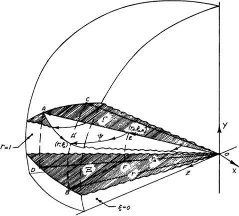
Thus in order to carry out the integrations the mapping of points on the shock wave to the vertical scale must first be determined. The Figure 2 shows the general situation with the vertical scale magnified to illustrate the mapping. In the figure, A is a typical point on the shock surface and A¹ is its

"image" point on the vertical scale ξ = .

One should be careful not to confuse the behavior of cross- flow streamlines with actual streamlines, particularly with re- gard to the continuity properties of actual streamlines. In using the concept of crossflow streamlines it is important to remember that the crossflow streamlines are actually the curves of intersections of stream surfaces, φ= constant, with the spherical surface,r= constant. Crossflow streamlines can therefore terminate in the flow field at crossflow stagnation points where the actual streamlines are in the radial direction.

Thus, in contrast to an actual two-dimensional flow, not every streamline that enters the shock layer upstream of a station

(e.g., station ξ^ξχ in Fig. 2) need cross that station.

Figure 3 shows the various surfaces and curves referred to in the previous discussion for a typical case. Tbe surfaces labeled

Γ , Ξ , and Ψ are the shock surface, the body surface and a typical stream surface, respectively. The curve E-A'lying in theW= constant surface is a typical three-dimensional stream- line, whereas the curves A-A'and F-B'are the "conical" and

"normal" projections of this streamline onto the spherical sur- face r= l and the body surface. By "conical" and "normal" is meant the projection along r and η coordinate lines respectively.

The arc C-B 'lying in the spherical surface, which shall be called the body normal, is the locus of points on the vertical scale corresponding to the body point B' (the vertical scale has again been magnified for purposes of discussion).

It is well known (Refs. 5> 6 and 7) that the streamlines play a particularly important role in the thin-shock-layer theory of general three-dimensional flows. The appearance of Newtonian shock lines in three-dimensional flows is an example of a three- dimensional phenomenon that is easily interpreted in terms of the streamline pattern on the developed surface. Therefore, in

any thin-shock-layer analysis of a three-dimensional flow there should he a careful study of the topological structure of the streamline in the shock layer. Such a study was undertaken by the present authors and is reported in Refs. 10 and U (a lengthier version of the present paper). Since the analysis of the streamline pattern is fairly lengthy and since it is fully discussed in the cited references, the present authors provide, without proofs, a description of some overall features of the crossflow streamline pattern.

Figure k, based on the analysis in Refs. 10 and 1 1 , gives a qualitative picture of the crossflow shock layer structure.

The notation corresponds to that used in Fig. 7 of Ref. 1 1 . The point to be stressed is that the crossflow streamlines do not terminate at a crossflow stagnation point, as one might ex- pect, but instead terminate at a crossflow stagnation surface, that is, a surface on which the crossflow velocity vanishes.

This surface is an envelope of the crossflow streamlines and consequently the entropy must be discontinuous across it. In addition, the slope of the lateral velocity distribution across the shock layer also jumps, as indicated in Fig. 5·

ENTROPY LAYER

In the previous sections it has been indicated how thin-shock- layer theory could be approached by the formal procedures of the theory of .asymptotic expansions. Also, the form was derived of the expansion appropriate for some as yet undefined regions of the shock layer. A simple analysis of the next terms in the series indicates that the region of validity of the outer solu- tion will, in general, not include the whole region of interest.

In this section, the regions of non-uniformity will be defined and the appropriate expansions, valid in these regions, deter- mined .

To illustrate clearly the basic nature of the non-uniformities, one need only investigate the analytic properties of the series representation for the function τ . The equation for τ is given by Eq. 9^ and is easily transformed into

(26a)

with G and H defined by

1 (26b)

G =

7 p q² Χξ^

and

- ^vi

H =

tan r Γ Π

K ' c o s r - - ! (26c)

*q L ^η q J

If the outer-solution expansions are substituted into Eq. 9b it is found that

.r<°> Dr' (0) + 1 and

and

p(0)^q(0)^{2 H}

v i0 )

The zeroth-order outer solution is given by

Dr<°>

+ 1 = 0

(27)

t a n r( 0 ) . _7i(0) ⁺H<0) _ (1) ^{t a n r}( 0 ) (28a) οξ ξ

•where

SCO L _ ^ (28b)

H(0) _ _JL_ w ^{s i n r}( 0 ) (28c)

q(0) ^b

(29a)

or

r^{( 0)} - 4 W - ξ (29b)

where

ή, -

i

W

Ά (29c)

Eq. 28a indicates a singularity at = 0 . Expanding the solu- tion of Eq. 56 about the zeros of r(0) obtains

r < » » G£°>

1α (ή,-ο

"where

G£>> . [5(0)] i m € b ( 3 0 b)

Therefore will have a logarithmic singularity at_the zeros of r ( ° ) if f 0. From Eq. 10 it can be seen that GJS>) is

zero only at symmetry planes. Thus the stagnation surfaces are loci of logarithmic singularities. It is concluded that the outer flow is not uniformly valid in the neighborhood of cross- flow stagnation surfaces. Higher-order terms of the series are even more strongly singular and the outer solution becomes com- pletely meaningless in these regions.

The appearance of a non-uniformity in the approximate solution indicates the presence of a term which, although negligible in the outer flow and uniformly small in the entire region, is capable of producing a first-order effect in regions where the non-uniformities are present_. From the previous analysis one can see_that the function f G is just such a term. It was shown that € G, which is essentially the pressure gradient, is neg- ligible in some region of the shock layer, including the shock wave and symmetry planes. The demonstration depended on the boundedness of the ratio of lateral pressure gradient to lateral velocity. Near the shock Ρ »Psand dPs/df taken along the shock is 0 ( v £ ). Thus the ratio is clearly bounded in a region which includes the shock wave. However as one moves across the shock layer along a body normal, many cases of a crossflow stagnation surface will be encountered. Since the lateral pressure grad- ient is in general not zero at these surfaces, the forementioned ratio is unbounded. The reasoning for the neglect of the pres- sure gradient term breaks down and the term must be retained in these regions. With the troublesome term identified one may determine its effect on the crossflow streamline pattern and develop the uniformly valid solution.

It is clear from the previous discussion that the pressure gradient term can have a first-order effect only in a region near the non-uniformity. As a result, it is expected that the outer solution will remain unchanged in most of the flow field but will be modified greatly near crossflow stagnation surfaces.

Within the zeroth-order approximation, the pressure gradient effects on an infinitely dense fluid are completely negligible and the streamlines terminate on a crossflow stagnation surface, which was shown to be an envelope of streamlines. However, if the density is large but finite, the lateral pressure gradient terms will cause a very low velocity flow along the stagnation surface. This slight lateral velocity causes substantial changes in the streamline behavior near these surfaces. With

ν ξ small but nonzero, the crossflow streamlines will no longer terminate on a specific surface but must terminate at a point determined by the conditions = θΡ/θξ=0. Since all the stream- lines will flow into this point, it is likely that this point is the nodal point singularity commonly referred to in the

literature as the "Ferri vortical singularity," The stagnation surface of the zeroth-order outer solution will most likely be- come, in a more accurate analysis of the entropy layer, the center of a finite region of low velocity crossflow. The stream- lines will probably be parallel and spaced close together, thus indicating large gradients of S , ρ , and v^f across the layer.

Before proceeding with the formal asymptotic analysis, it will be instructive to consider the apparent difference between the entropy layer of the thin-shock-layer analysis and the now familiar entropy layer associated with conical perturbation theories. In these latter theories, the lateral pressure grad- ient terms are retained in the first-order analysis, but the crossflow streamline shapes are approximated by body normals;

the actual streamlines are assumed to deviate only slightly from this basic, axial,1 y symmetric pattern. However, near the body surface the exact streamlines are parallel to the body surface and the perturbation solution exhibits logarithmic singularities indicating the occurrence of non-uniformities.

The singular behavior is, in this case, directly attributable to the approximation of the streamline shapes near the body sur- face. In the hypersonic case, no approximations involving streamline shapes are introduced and the non-uniform behavior of the solution is caused solely by the neglect of the lateral pressure gradient term. Cheng (Ref. k) in his analysis of the entropy layer considered both effects but did not note any dis- tinction in the way the basic parameters, a the angle of attack, and € enter irito the solution. However the procedure of treat- ing both effects simultaneously probably masked any possible differences.

In the remaining part of this paper a rational theory of hyper- sonic entropy layers is developed using two different approaches.

In the first method the problem is treated by the boundary layer techniques of Carrier (Refs. 12 and 1 3) , and then the same prob- lem is treated by Lighthill1s technique for rendering approxi- mate solutions to physical problems uniformly valid (Refs. Inl-

and 1 5 ) · The boundary layer method is more closely related to the physics of the problem and it expresses the solution in a form which clearly exhibits the fundamental nature of the singu- larity. Lighthill1 s method, although more abstract then the boundary layer theory, is more systematic and better suited for determining the higher-order terms in the expansions. In addi- tion Lighthill1s approach yields a solution in a form better suited for numerical application. In this preliminary investi- gation the present authors are concerned only with the problem of obtaining the simplest uniformly valid solution and not with the development of a complete theory, valid to any order.

Therefore, in general, only the first terms in the various ex- pansions are considered.

In the section dealing with outer flow, it was seen that the first step in the solution was the determination of the lateral velocity , or equivalently the "lateral angle" τ . The low- est-order solution for τ was found by neglecting the effects of the lateral pressure gradient terms on r · In the previous dis- cussion it was seen that this step led to non-uniformities in certain regions of the flow field. Thus it appears that the question of non-uniforaiity is closely linked to the determina- tion of the variable r .

Equation 27 provides two possible solutions for , one of which has already been discussed. This solution (Eq. 29a), was shown to be valid in a region including the shock but was

singular near surfaces where r ( ° ) = 0. The second possible solu- tion to Eq. 27 was found to be r ( ° ) = 0, and thus in this inves- tigation of non-uniformities one is led quite naturally to ex- amine the expansions derived from this solution. An expression for r is assumed in the form

r = ΓΓ < ° > + . . . (31)

i

and the subscript i indicates "inner solution." Substituting Eq. 31 into Eq. 26a brings

r<°> = - G <0> = - - 1 (32)

1 pj0) q.(0)2 Βξ

using Eq. 28b. It is noted that p/0) , q/0) and P /0 ) must be determined in order to complete the solution for r . ( ° ) . Leav- ing this question for the moment and assuming that these quan- tities can be determined, the "matching" of the inner and outer solutions is next investigated.

To prove that two solutions match it must be shown that:

l) they have a common region of validity; and 2) they are asymp- totically equivalent in their common range of validity. On the basis of the last of these two conditions, it is obvious that the two solutions obtained thus far do not match. To illustrate, one may refer to Fig. 6, in which is is seen that these solutions intersect but with discontinuous slope. Thus the first terms of the expansions can not be asymptotically equivalent in any common range. This is to be expected for at least two reasons:

The scale of the independent variable is the same in each region, and secondly there is no free constant (or more accurately no free function of φ ) with which to effect the matching.

The matching problem can be treated by two fundamentally dif- ferent approaches, one based on the inner solution and the sec- ond based on the outer solution. In each of these procedures

the main idea is to extend the range of validity of one of the two basic solutions so that it overlaps the range of validity of the other. In working from the inner flow one is faced with a classical singular perturbation problem in which the highest- order derivative is dropped in each stage of the analysis. The reduction of the order of the differential equation results in a reduction of the number of possible boundary conditions that can be satisfied. In the present case a first-order differential equation is reduced to an algebraic equation and the number of boundary conditions that can be satisfied is reduced from one to zero. This explains, in mathematical terms, the lack of freedom in the matching problem. The problem is solved in this approach by application of Carrier1s boundary layer techniques which were designed to treat problems of the general type just outlined.

The method used in the second approach is closely linked to the mode of failure of the outer solution. In studying the be- havior of the outer solution, it was seen that the first-order term had a logarithmic singularity at ξ Investigation of the higher-order terms of the expansion indicated am even more singular behavior at ξ=ξ\^> . The ratio of successive terms can be shown to be unbounded in the neighborhood of the singular point. This divergence of the expansion can be avoided by modifying the expansion procedure as indicated by P.L.K, method

(Refs. Ik and 15 ) .

In Carrier's method an arbitrary stretching of dependent and independent variables is introduced. The stretching factors are defined by the conditions that the highest-order derivative is retained in the lowest approximation and that the new,

stretched coordinate is measured from the point of application of the boundary condition. In the present case there is a matching condition instead of a boundary condition, and it will be sufficient to measure the stretching variable from the point

The stretched variable is therefore defined by the re- lations

r = 7a7 (33a)

ξ - fb - ? b ? (33b)

The condition that the highest-order derivative be retained leads to

a = b (3IO

Substituting Eqs. 33 into 26a and making use of Eq. 3^, one finds

taD(€

7)iJBL+ χ I = 7 ( H - G) χ. (35)

The coefficient a is determined by the condition that the solu- tion match with the inner solution. This leads to

a - b - 1 (36)

with the result that

+ χ Α - ( H -

G )v

From Eq. 26c it is seen that

Η = 0(r) = 0 (77)

and Η is negligible to the order considered. In addition one obtains from Eq. 16

χξ - ι + 0(O

so that the final equation for the matching or "transition"

solution is given by

7(0) ^{+ 1} . _ g < ° > (37)

where the superscript 0 again denotes the lowest-order solution.

One further simplification results by introducing the coordin- ate stretching, Eq. 33, into the equation for G ^# Thus consid- ering G as a function of ξ for fixed ψ

G(f,7) = G ( ? , 4,7)

Since

it is found that

lim G( £ fb, 0 - G (f^b,0) for J fixed (38) and the function G ^ may be replaced by the constant g£°^ which

is equal to the value of at ξ = £^b · Therefore

- - « £ • » ^{) ( 3 9}

from vhich

7(0) - Gg») ^{l n} (-(0) ⁺ = _ J + c ^{( ψ)} where c is an arbitrary function of φ .

The matching conditions for the inner flow take the form

lim 7(°> = lim r j^{0 )} (In)

Expansion of the inner solution (Eq. 6 0 ) about f=£b yields

r(.^{0) =} _ G t^{0 )} + ^{0 ( 4 -} ξ) (tea)

Similar expansion of the transition solution (Eq. kO) for ξ-*-*»

(

The matching condition therefore requires that both error terms vanish simultaneously in the limit *-»0 (or ξ·* This condi- tion is obviously satisfied for any ξ in the region

f - fb - 7° 0 < η < 1

It is noted that the matching of the inner and transition solu- tions does not impose any condition on the arbitrary function

c ( φ ). Thus the transition solution adds the freedom required for matching to the outer flow. In order to match the transi- tion solution to the outer flow and thereby to fix the arbitrary function c ( φ ) , one first writes the transition solution in terms of the variables of the outer solution. Thus Eq. hO be- comes

r(o) _ TG^O) [LN ( R( 0 ) ⁺

_

7 ] .

_

Thus if c is chosen so that

c = - G£ ° > I n ? ( * 5 )

then

r<°> - $ , - £ + 0(7)

Consequently the transition and outer solutions match in the whole outer region with an error of 0 ( 7 ) · With c defined by Eq. 4-5, the transition solution becomes

It may be noted that the solution for r^t is given implicitly by Eq. kj. Although Eq. k'J clearly exhibits the nature of the singularity, its form greatly complicates the completion of the full zeroth-order uniformly valid solution.

On the basis of the foregoing discussion it is clear that the solution must behave as indicated in Fig. 6. In this repre- sentation the transition region is a mathematical boundary layer across which the derivative dr/άξ rapidly changes in magnitude.

By the use of Carrier's boundary layer technique, a uniformly valid solution for r(0) is obtained by splitting the flow field into three regions and finding the appropriate expansion valid in each. The solutions were shown to match but because of the implicit form of the transition solution, uniformly valid solu- tions for the other variables were not derived. In this sec- tion the P.L.K, method is applied to develop a representation for r ( ° ) that will bring a complete solution in a compact form.

The use of this general method could not obtain a single repre- sentation uniformly valid in the whole region. As shall be seen, a separate solution for the inner flow is still required.

In the P.L.K, method both dependent and independent variables are expressed in terms of an auxiliary variable and are expanded in powers of 7 . This introduces a degree of freedom into the problem which can be used to control, to some extent, the behav- ior of the expansions near the singularity. When the P.L.K, method is successful, both sets of expansions can be made to converge in the neighborhood of the singular point.

The authors next consider the behavior of the solution to Eq.

26a with tan r approximated for small τ and χ. approximated by the first term in its series development

(Vr)

where the subscript ο denotes outer flow. If

where

then

d"o - _

(ξ + €τ0) = G - H = ι(ξ) (1|β)

άξ

which is exactly in the form of one of the cases treated by Lighthill in (Refs. Ik and 15)· Eq. kd clearly indicates the applicability of the P.L.K, method to the present problem. In fact since the singularity occurs at = 0, the approximations on tanr introduces only higher order effects, and solutions to Eq. 4 8 would yield valid first-order results in the neighbor-*

hood of the singularity.

In the present investigation it is convenient to use Temple's method of regularization (Ref. 16) to obtain the P.L.K, expan- sions. To apply this method Eq. 26a is written as

Dr - [ t a n r + €j]x^

Όξ tan r

where the term G-Hhas been replaced with J and the subscript ο has been dropped, since no confusion will arise. Next the auxiliary variable ζ and an arbitrary function f ( ζ ) is intro- duced, and the foregoing equation is split into the equivalent system

Dr

f ( z ) = - [ t a n r + e J ]

f ( z ) Dz

Όξ tan r

The f ( ζ ) is chosen so that the expansions for r and ξ start with the terms and ζ . Thus

f ( z ) = t a n r( 0)

The governing system of equations become

t a n r(0) .El ^ä _ [ t a n r + 7 j ] (49a)

Dz

t a n r( 0 ) EL . (k9b) Dz γ

ξ

If all the variables are expressed in the series form indi- cated by Eqs. 15-17> it becomes possible to express the func- tion J as

Τ = T( n) (50a)

η = o

The following series development is introduced for ξ

(50b)

η = 0

The and χ/η^ are in general known functions of ξ at each stage of the solution and must be expressed in terms of ζ to proceed. For each j(n) and χ ^ the following expansions are valid ^

7 0 » ^{( a} . J ( n )^{( 2 ) +} j ^ ( D ⁺ . . . (51)

dz dX(n) (Z)

χ[^η)(ξ) = x i^{n )}( z ) + 7 —1 f < »⁺. . . (52) f £ dz

Substituting the foregoing expansions and the expansions in Eqs. I 5 - I 7 into Eqs. 49 brings

+ 1 = 0 (53a)

Dz

D£ W _^{= i} (53b)

Dz

( 0 ) D r < » r < » - ( 0 ) , . (530) tan r ' + -— = - J ( z )

»z c o s2 r<°>

ο ^ ω r œ_xa)^{s i n r}( o )^{c o s r}( o ) (53d)

0 2 = . i n r < ° > c o . r « >