Accepted manuscript of the paper Cite as:
Tamás Bozóki, Ernő Prácser, Gabriella Sátori, Gergely Dálya, Kornél Kapás and János Takátsy, 2019:
Modeling Schumann resonances with schupy, Journal of Atmospheric and Solar-Terrestrial Physics, Volume 196, 105144, https://doi.org/10.1016/j.jastp.2019.105144
© 2019. This manuscript version is made available under the CC-BY-NC-ND 4.0 license http://creativecommons.org/licenses/by-nc-nd/4.0/
Research Paper
Modeling Schumann resonances with schupy
Abstract
Schupy is an open-source python package aimed at modeling and analyzing Schumann resonances (SRs), the global electromagnetic resonances of the Earth-ionosphere cavity resonator in the lowest part of the extremely low frequency band ( 100 Hz). Its very-first function forward_tdte applies the solution of the 2-D telegraph equation obtainedintroduced recently by Prácser et al. (2019) for a uniform cavity and is able to determine theoretical SR spectra for arbitrary source-observer configurations. It can be applied for both modeling extraordinarily large SR-transients or
“background” SRs excited by incoherently superimposed lightning strokes within an extended source region. Three short studies are presented which might be important for SR related research.
With the forward_tdte function our aim is to provide a medium complexity numerical background Tamás Bozókia,b,∗ bozoki.tamas@csfk.mta.hu, Ernő Prácsera, Gabriella Sátoria, Gergely Dályac, Kornél Kapásc, János Takátsyc
aResearch Centre for Astronomy and Earth Sciences, Geodetic and Geophysical Institute, Csatkai Endre utca 6-8, Sopron H-9400, HungaryGeodetic and Geophysical Institute, Research Centre for Astronomy and Earth Sciences, Csatkai Endre utca 6-8, Sopron H-9400, Hungary
bSchool of Environmental Sciences, University of Szeged, Aradi vertanuk tere 1, Szeged H-6720,
HungaryDoctoral School of Environmental Sciences, University of Szeged, Aradi vertanuk tere 1, Szeged H-6720, Hungary
cEotvos Lorand University, Pazmany Peter stny. 1/A, Budapest H-1117, Hungary
∗Corresponding author. Research Centre for Astronomy and Earth Sciences, Geodetic and Geophysical Institute, Csatkai Endre utca 6-8, Sopron H-9400, Hungary.
∗Corresponding author. Geodetic and Geophysical Institute, Research Centre for Astronomy and Earth Sciences, Csatkai Endre utca 6-8, Sopron H-9400, Hungary.
Author has made corrections in ce:affiliation. Carry out the corrections in sa:affiliation also using the XML Editor.
for the interpretation of SR observations. We would like to encourage the community to join our project in developing open-source analyzing capacities for SR research as part of the schupy package.
Keywords: Schumann resonances; Earth-ionosphere cavity; Numerical model; Python package
1.
Introduction
Schumann resonances (SRs) are the global electromagnetic resonances of the Earth-ionosphere cavity, characterized by peak frequencies of about 8, 14, 21, 26 etc. Hz (Balser and Wagner, 1960; Galejs, 1972;
Madden and Thompson, 1965; Nickolaenko and Hayakawa, 2002; Price, 2016; Sátori, 1996; Schumann, 1952;
Wait, 1996). They are known as a powerful tool for monitoring lightning activity on regional and global scales (Boldi et al., 2018; Dyrda et al., 2014; Sátori and Zieger, 1999; Williams and Sátori, 2004) and also as an important source of information about the global state of the lowest part of the ionosphere (Dyrda et al., 2015;
Kudintseva et al., 2018; Nickolaenko et al., 2012; Roldugin et al., 2003, 2004; Sátori et al., 2016; Shvets et al., 2017; Williams and Sátori, 2007). Recently, a major interest arose for SRs in connection with gravitational wave detection (Coughlin et al., 2016, 2018; Kowalska-Leszczynska et al., 2017).
BasicallyEssentially, it is the very weak attenuation rate (about 0.5 dB/Mm, Chapman et al., 1966; Wait, 1996) of electromagnetic (EM) waves in the lowest part of the extremely low frequency band ( 100 Hz) that enables the formation of SRs. Lightning radiated EM waves can travel a number of times around the globe before losing most of their energy and the constructive interference of the waves propagating in the opposite directions (direct and antipodal waves) forms the resonance structure. Most of the lightning strokes formare part of a quasi-steady “background” field from where individual lightning discharges cannot be distinguished, while there also exist extremely large excitation events known as SR-transients or Q-bursts (Boccippio et al., 1995; Guha et al., 2017; Ogawa et al., 1967) which largely exceed the “background”s signal strength.
In the last decades several approaches have been published about the numerical modeling of SRs with various complexity (Kulak et al., 2003b; Kulak and Mlynarczyk, 2013; Morente et al., 2003; Toledo-Redondo et al., 2016; Yang and Pasko, 2006). Many of them were applied with great success to understand peculiar observational phenomena (e.g. Kudintseva et al., 2018; Kulak et al., 2003a; Yang and Pasko, 2006, 2007). On the other hand there are observations where detailed numerical interpretations are still desired (e.g. Sátori, 1996; Satori, 2003; Satori and Zieger, 2003). In order to facilitate such kind of scientific objectives here we present a new python function forward_tdte which is capable of modeling the theoretical SR spectraum for arbitrary source-observer configurations with medium complexity. The basis of the code is the forward modeling part of Prácser et al. (2019) rewritten in python. This function is part of the newly established open- source python package callednamed schupy. In Section we introduce the applied 2-Dtwo-dimensional telegraph equation (TDTE) framework. Following that, we describe the schupy package and the forward_tdte function in Section and then carry out three short studies in Section . Finally, we summarize our main conclusions in Section .
2.
Theoretical background
2
3 4
5
The theoretical description of SRs is most naturally formulated in spherical coordinates (r, ϑ, φ). The radius of the inner boundary, the Earth's surface, is denoted by R and the height of the ionosphere by h. Furthermore, we use the following notation conventions:
• standard physical quantities (i.e. voltages, V, currents, I, admittances, Y, etc.) are denoted by capital letters,
• the surface densities of the same quantities are denoted by calligraphic letters (e.g. , ),
• while linear densities are denoted by lowercase letters (e.g. i).
During our derivation we assumeuse the fact that the time evolution of the solution can be separated from its spatial dependence, and takes the form of with various ω frequencies, where j is the imaginary unit.
We assume that the Earth-ionosphere waveguide can be modeled as a 2-D transmission line ( Fig. 1 ) which is a valid approximation, as the wavelengths of the guided waves are much longer than the distance between the Earth's surface and the ionosphere. In a local treatment the transmission surface can be represented by elementary circuit components. These elementary components can be described by four quantities, namely (admittance) and (impedance), where C and L denote the capacitive and the inductive elements, respectively, and can be expressed in the following general form:
where G is the conductance, B is the susceptance, R is the Ohmic resistance, and X is the reactance.
(1)
Fig. 1
From charge conservation on the surface the divergence of the surface current density vector in the ionosphere can be written as:
where is the current density of the source and V is the electric potential between the ionosphere and the Earth's surface. An additional equation can be obtained from the differential Ohm's law:
It follows that the natural variables of the TDTE approach are the voltage (V) and the surface current density vector ( ), while the electric and magnetic field components can be expressed as:
from V and (Madden and Thompson, 1965 ).
If we assume, that the surface of the Earth and the ionosphere are perfect conductors and there is vacuum between them, then:
where and denotes the capacitance and inductance, respectively.
In addition, we also assume, that the impedance and admittance are constants on the surface, i.e. we have a uniform Earth-ionosphere cavity. In this case Eqs. (2) and (3) can be combined to arrive at the telegraph equation:
Circuit network of the 2-D transmission line (from Madden and Thompson, 1965). The inductive elements cover the ionosphere while the capacitive elements connect it with the Earth's surface.
(2)
(3)
(4)
(5)
(6)
(7)
In order to find the solution for this equation, first we assume, that the source term can be described by a vertical Dirac-δ current impulse (representing a single lightning stroke) and construct our coordinate system in a way that its North Pole coincides with the position of the source. Since the source is symmetric under rotations around the vertical axis in this case, the solution will be independent of the coordinate φ. A general potential on the surface of a sphere can be expressed as a linear combination of spherical harmonics. Due to rotational symmetry the solution can be expressed in the form:
where is the Legendre polynomial of degree n. The Laplacian acts on the Legendre polynomials as
where R is the radius of the sphere. Note, that by exchanging the variable ϑ to we arrive at Legendre's equation, which is the defining equation of the Legendre polynomials. The source term can also be expressed using Legendre polynomials (see e.g. Bronshtein and Semendyayev, 1997 , on the completeness of Legendre polynomials):
where I is the total current, which we get when integrating for the surface of the sphere. Inserting Eqs. (8) and (10) into Eq. (7) and using Eq. (9) we arrive at
Since the Legendre polynomials are linearly independent the solution can only be achieved trivially, i.e. when all coefficients are 0. Hence, solving for and inserting it back into Eq. (8) we get:
(8)
(9)
(10)
(11)
where we introduced the notation , which is the current moment of the lightning source. This way M becomes the source quantity, which is more suitable for generalized uses. As stated in Prácser et al. (2019) by using Eqs. (3) and (4) this formula gives the same expression for the EM field components as in e.g. Galejs (1972) ; Mushtak and Williams (2002) ; Nickolaenko and Hayakawa (2002) ; Wait (1996) .
The generalized formula for arbitrary ( ) source and ( ) observation locations can easily be acquired by replacing with , where γ is the angle between the source and observation positions, and can be expressed in the following form:
Using Eqs. (3) and (4) and the relation , one can derive expressions for the components of magnetic induction:
Using these expressions and Eq. (4) we can obtain the general equations for , , :
where d d [Instruction: To DC: Delete the last math
only]are the first order associated Legendre polynomials. These equations were first published recently by (12)
(13)
(14)
(15)
(16)
(17)
Prácser et al. (2019) and can be regarded as the generalization of the formalism introduced in the PhD thesis of Nelson (1967).
In a more realistic scenario the resistance of the ionosphere and the conductance of the air are not equal to zero as it has been assumed in Eqs. (5) and (6). However simply assigning them nonzero values the elegant analytical formalism of Eqs. (15)–(17) would not hold anymore. Therefore, following the method of Kirillov and Kopeykin (2002), we take the losses into account by introducing two complex equivalents for the altitudes of the transmission line and , defined by the following relations (see Madden and Thompson, 1965;
Greifinger and Greifinger, 1978; Mushtak and Williams, 2002):
where
It follows that the capacitive admittance and the inductive impedance is also modified:
and hence, the following relation holds:
Thus, in Eq. (12) and all other equations that follow from this one, h is replaced by , and Eq. (21) has to be inserted in the denominator. In case of and these heights simply become h. About the determination of and see e.g. Kulak and Mlynarczyk (2013) or Mushtak and Williams (2002) .
For the evaluation of the (associated) Legendre polynomials in practical applications (Eqs. (15)–(17) ), it is convenient to use the following recursive formula:
(18)
(19)
(20)
(21)
(22)
where , and . Using this relation, we only need the first few Legendre polynomials, namely
, , , and .
In order to consider multiple sources the summed effect of each source has to be calculated. Since the superimposed lightning strokes are incoherent in nature their power spectral densities have to be used for the summation (e.g. Nickolaenko et al., 1996). It follows, that the unit of the source term is C2km2/s corresponding to electric and magnetic spectra in mV2/m2/Hz and in pT2/Hz, respectively.
3.
Package description
The schupy package contains a modeling function at its current release, named forward_tdte, which simulates SRs generated by an arbitrary distribution of lightning sources specified by the user and returns the theoretical electric and magnetic fields at the user-specified location.
The schupy package can simulate point sources as well as extended ones. It is possible to specify the size of the extended source, which the code will represent as randomly distributed point sources within the given radius from the center of the source that, which haves a total intensity specified by the user (as an example see Fig. 2). The method of the height calculation can be set either to “mushtak” corresponding to the model of Mushtak and Williams (2002) or to “kulak” corresponding to the model of Kulak and Mlynarczyk (2013).
Geographic locations of the sources and of the observing station can be visualized by schupy, making use of the cartopy package for visualization of the Earth. 1
The schupy package is available via the pip package manager system (https://pypi.org/project/schupy/) and the project's Github page: https://github.com/dalyagergely/schupy, where a more detailed technical description is presented as well..
Fig. 2
Map of an extended source at (radius = 1 Mm).
4.
Short studies based on schupy.forward_tdte
In this section we present three short studies based on schupy.forward_tdte which might be interesting for SR related research. First, we test the convergence of theoretical spectra, then we compare the spectra generated by two antipodal sources, and finally the difference between the spectra of point and extended sources is investigated. The function calls that we used for the short studies are provided in the Appendix[Instruction: To DC: link to Appendix]. of the paper.
4.1. Convergence of theoretical spectra
As it can be seen in Eqs. (15)–(17) the electromagnetic field components of SRs arecan be calculated as an infinite sumsmation of (associated) Legendre-polynomials. Practically, only a finite number of summation can be done (up to n), thus the question arises: at what n can we accept the result? It is to be noted, that the answer depends on the source-observer distance.
In order to investigate this problem we carry out a test where the (lat,lon) positions of a point-like lightning
source with source intensity are: , , ,
, and , respectively and the theoretical
spectra are determined for the location in each case. The theoretical spectra are calculated for the
Fig. 3
Convergence of the theoretical spectra for the component for different source-observer distances. n denotes the maximal order of Legendre-polynomials included in the summationto sum.
following values of n: [10, 50, 100, 500, 1000, 5000]. All the positions are on the Equator, therefore the component is always zero. The results are shown in Figs. 3 and 4.
It can be noted that converges faster than . Our conclusion is that in most cases should be enough except when calculatingfor withwhen the observer is close to the source ( ).
4.2. Theoretical spectra of antipodal sources
This test is devoted to compareing theoretical spectra of antipodal sources. Here, our motivation is to gain more insight about non-uniqueness, which manifests as parallel equivalent solutions for the SR inversion task (see e.g. Prácser et al., 2019 ). In a lossless cavity antipodal sources would produce exactly the same spectra at arbitrary location on Earth. However the Earth-ionosphere cavity is lossy, which is taken into account by introducing and complex equivalents of the altitudes. The question is, in what extent does the theoretical spectra differ in this formalism.
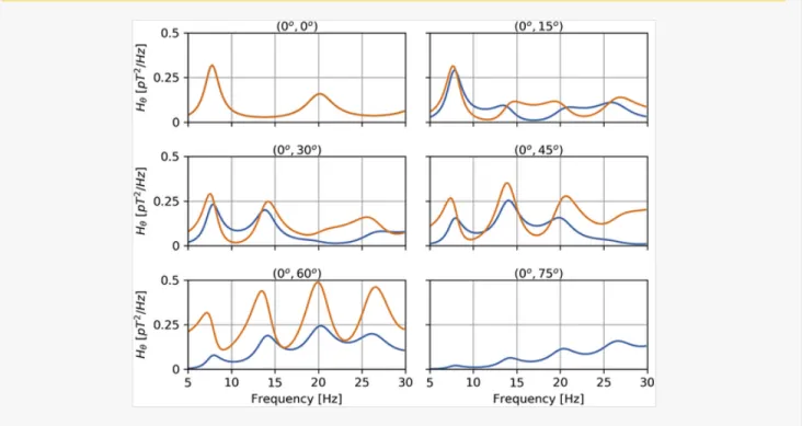
We place two sources with the same intensities of at antipodal positions and and determine the theoretical spectra for the following locations: , , , , and . As in the previous test, all the positions are on the Equator, therefore the component is always zero.
Fig. 4
The same as Fig. 3 but for the component. Note, that the upper limit of the y axis is different for the two shortest source- observer distances than for the other cases.
It can be seen that in the midpoint the theoretical spectra are exactly the same (Figs. 4 and 5Figs. 5 and 6)[Instruction: To DC: Figs. 5 and 6 floatanchor here], however apart from this specific point the two spectra are noticeably different (see Fig. 6).
4.3. Point versus extended source
In this test we compare the theoretical spectra of a point source with thatose of an extendeddistributed source (with a radius of 1 Mm). Both the centroid position of the extended source and the location of the point source are , and we determine the theoretical spectra for the equatorial distances of , , , , and . The extended source consists of 100 randomly distributed sources within the given radius with a total intensity of , the same value as set for the point source. Fig. 7 shows the relative difference of the two cases, defined as
where S denotes the theoretical spectrum (either or ). As in the previous two studies, is always zero.
Fig. 5
Theoretical spectra of the component for the two antipodal sources at different observer positions. The orange and the blue lines mark the theoretical spectra of the sources at and , respectively.
(23)
Fig. 6
Replacement Image: H_theta_all.png
Replacement Instruction: To graphics: Replace image requested. The ylabel was wrong on the previous version.
It can be noted that the further the source is the larger the relative difference between the field generated by the two kinds of sources becomes. As it can be expected the most noticeable differences can be found at the nodal points of the resonance field.
Figure Replacement Requested
The same as Fig. 5 but for the component.
Fig. 7
The relative difference between the theoretical spectra of a point and an extendeddistributed (radius = 1 Mm) source.
5.
Summary
• In this paper we introduced our newly established open-source python package schupy and its very-first function forward_tdte for SR modeling, which enables to calculatinge the theoretical SR spectra for arbitrary source-observer configurations.
• The package can be downloaded via pip and the source code is freely available on Github.
• We have carried out three short studies where we investigated the convergence of the theoretical spectra, the theoretical spectra of antipodal sources and the theoretical spectra of an extended distributed source.
• We encourage the community to join our initiation and participate in developing open-source analyzing capacities for SR research as part of the schupy package.
Acknowledgements
The authors would like to acknowledge the very valuable and fruitful discussions with Earle Williams on the topic of this paper. Special thank concerns We thank Anirban Guha that hewho enabled the comparison of the present model with the SR model developed at MIT. The MIT effort in Schumann resonances has been generously supported by Grainger Foundation. We are thankful to István Bozsó for his helpful comments on the code. The work of T. Bozóki and G. Dálya was supported by the ÚNKP-198-3 New National Excellence Program of the Ministry of Human Capacities. T. Bozóki was supported by the COST Action CA15211. The contribution of G. Sátori was supported by the National Research, Development, and Innovation Office, Hungary-NKFIH, K115836, and also by the COST Action CA15211.
Appendix
Additionally, we would like to provide some support for readers aiming to reconstruct the three short studies presented in this article. First, forward_tdte function and numpy should be imported with the following commands: from schupy import forward_tdte, import numpy as np.
• The convergence of theoretical spectra can be tested with the following piece of code:
Previous Version
Updated Version
, where the source distance is 10[Instruction: To DC: 10 (deg sign)] and the summation is done up to 500 in this case.
• the theoretical spectra of antipodal sources with:
,where the observer position is (0,15) in this case.
• and the relative difference between the theoretical spectra of a point and an extended distributed source with:
, where the observer position is (0,15) in this case.
References
i The corrections made in this section will be reviewed and approved by journal production editor.
Previous Version
Updated Version
Previous Version
Updated Version
Chapman, F.W., Jones, D.L., Todd, J.D.W., Challinor, R.A., 1966. Observations on the propagation constant of the earth ionosphere waveguide in the frequency band 8 c/s to 16 kc/s. Radio Sci. 1, 1273–
1282.
Coughlin, M.W., Christensen, N.L., Rosa, R.D., et al., 2016. Subtraction of correlated noise in global networks of gravitational-wave interferometers. Class. Quant. Gravity 33, 224003.
Kulak, A., Ziba, S., Micek, S., Nieckarz, Z., 2003. Solar variations in extremely low frequency propagation parameters: 1. a two-dimensional telegraph equation (tdte) model of elf propagation and fundamental parameters of schumann resonances. J. Geophys. Res.: Space Phys. 108.
Madden, T., Thompson, W., 1965. Low-frequency electromagnetic oscillations of the earth-ionosphere cavity. Rev. Geophys. 3, 211–254.
Morente, J.A., Molina-Cuberos, G.J., Portí, J.A., et al., 2003. A numerical simulation of earth’s electromagnetic cavity with the transmission line matrix method: schumann resonances. J. Geophys.
Res.: Space Phys. 108.
Balser, M., Wagner, C.A., 1960. Observations of earth-ionosphere cavity resonances. Nature 188, 638–
641.
Boccippio, D.J., Williams, E.R., Heckman, S.J., et al., 1995. Sprites, elf transients, and positive ground strokes. Science 269, 1088–1091.
Boldi, R., Williams, E., Guha, A., 2018. Determination of the global-average charge moment of a lightning flash using schumann resonances and the lis/otd lightning data. J. Geophys. Res.: Atmos. 123, 108–123.
Bronshtein, I.N., Semendyayev, K.A., 1997. Handbook of Mathematics. third ed. Springer-Verlag, Berlin, Heidelberg.
Coughlin, M., Cirone, A., Meyers, P., et al., 2018. Measurement and subtraction of schumann resonances at gravitational-wave interferometers. Phys. Rev. D 97.
Dyrda, M., Kulak, A., Mlynarczyk, J., et al., 2014. Application of the schumann resonance spectral decomposition in characterizing the main african thunderstorm center. J. Geophys. Res.: Atmos. 119, 13,338-13,349.
Dyrda, M., Kulak, A., Mlynarczyk, J., Ostrowski, M., 2015. Novel analysis of a sudden ionospheric disturbance using schumann resonance measurements. J. Geophys. Res.: Space Phys. 120, 2255–2262.
Galejs, J., 1972. Terrestrial Propagation of Long Electromagnetic Waves, International Series of Monographs on Electromagnetic Waves. Pergamon Press.
Greifinger, C., Greifinger, P., 1978. Approximate method for determining elf eigenvalues in the earth- ionosphere waveguide. Radio Sci. 13, 831–837.
Guha, A., Williams, E., Boldi, R., et al., 2017. Aliasing of the schumann resonance background signal by sprite-associated q-bursts. J. Atmos. Sol. Terr. Phys. 165–166, 25–37.
Kirillov, V.V., Kopeykin, V.N., 2002. Solving a two-dimensional telegraph equation with anisotropic parameters. Radiophys. Quantum Electron. 45, 929–941.
Kowalska-Leszczynska, I., Bizouard, M.-A., Bulik, T., et al., 2017. Globally coherent short duration magnetic field transients and their effect on ground based gravitational-wave detectors. Class. Quant.
Gravity 34, 074002.
Kudintseva, I.G., Galuk, Y.P., Nickolaenko, A.P., Hayakawa, M., 2018. Modifications of middle atmosphere conductivity during sudden ionospheric disturbances deduced from changes of schumann resonance peak frequencies. Radio Sci. 53, 670–682.
Kulak, A., Mlynarczyk, J., 2013. Elf propagation parameters for the ground-ionosphere waveguide with finite ground conductivity. IEEE Trans. Antennas Propag. 61, 2269–2275.
Kulak, A., Kubisz, J., Michalec, A., Ziba, S., Nieckarz, Z., 2003. Solar variations in extremely low frequency propagation parameters: 2. observations of schumann resonances and computation of the elf attenuation parameter. J. Geophys. Res.: Space Phys. 108.
Mushtak, V.C., Williams, E.R., 2002. Elf propagation parameters for uniform models of the earth–
ionosphere waveguide. J. Atmos. Sol. Terr. Phys. 64, 1989–2001.
Nelson, P., 1967. Ionospheric Perturbations and Schumann Resonance Data, PhD Thesis MIT, Project NR–371–401, Geophysics Lab. MIT, Cambridge Mass.
Nickolaenko, A., Hayakawa, M., 2002. Resonances in the Earth-Ionosphere Cavity, Modern Approaches in Geophysics. Springer Netherlands.
Nickolaenko, A., Hayakawa, M., Hobara, Y., 1996. Temporal variations of the global lightning activity deduced from the schumann resonance data. J. Atmos. Terr. Phys. 58, 1699–1709.
Nickolaenko, A.P., Kudintseva, I.G., Pechony, O., et al., 2012. The effect of a gamma ray flare on schumann resonances. Ann. Geophys. 30, 1321–1329.
Ogawa, T., Tanaka, Y., Yasuhara, M., Fraser-Smith, A.C., Gendrin, R., 1967. Worldwide simultaneity of occurrence of a q-type elf burst in the schumann resonance frequency range. J. Geomagn. Geoelectr. 19, 377–384.
Prácser, E., Bozóki, T., Sátori, G., et al., 2019. Reconstruction of global lightning activity based on schumann resonance measurements: model description and synthetic tests. Radio Sci. 0.
Price, C., 2016. Elf electromagnetic waves from lightning: the schumann resonances. Atmosphere 7.
Roldugin, V.C., Maltsev, Y.P., Vasiljev, A.N., Shvets, A.V., Nikolaenko, A.P., 2003. Changes of schumann resonance parameters during the solar proton event of 14 july 2000. J. Geophys. Res.: Space Phys. 108.
Roldugin, V.C., Maltsev, Y.P., Vasiljev, A.N., Schokotov, A.Y., Belyajev, G.G., 2004. Schumann resonance frequency increase during solar x-ray bursts. J. Geophys. Res.: Space Phys. 109.
Sátori, G., 1996. Monitoring schumann resonances-ii. daily and seasonal frequency variations. J. Atmos.
Terr. Phys. 58, 1483–1488.
Satori, G., 2003. On the dynamics of the north-south seasonal migration of global lightning. In:
Proceeding of the 12th ICAE, Global Lightning and Climate. pp. 1–4.
Sátori, G., Zieger, B., 1999. El nino related meridional oscillation of global lightning activity. Geophys.
Res. Lett. 26, 1365–1368.
Satori, G., Zieger, B., 2003. Areal variations of the worldwide thunderstorm activity on different time scales as shown by schumann resonances. In: Proceeding of the 12th ICAE, Global Lightning and Climate. pp. 1–4.
Sátori, G., Williams, E., Price, C., et al., 2016. Effects of energetic solar emissions on the earth–
ionosphere cavity of schumann resonances. Surv. Geophys. 37, 757–789.
Schumann, W.O., 1952. Über die strahlungslosen Eigenschwingungen einer leitenden Kugel, die von einer Luftschicht und einer Ionosphärenhülle umgeben ist. Zeitschrift Naturforschung Teil A 7, 149–
154.
Shvets, A.V., Nickolaenko, A.P., Chebrov, V.N., 2017. Effect of solar flares on the schumann-resonance frequences. Radiophys. Quantum Electron. 60, 186–199.
Toledo-Redondo, S., Salinas, A., Fornieles, J., Portí, J., Lichtenegger, H.I.M., 2016. Full 3-d tlm simulations of the earth-ionosphere cavity: effect of conductivity on the schumann resonances. J.
Geophys. Res.: Space Phys. 121, 5579–5593.
Wait, J., 1996. Electromagnetic Waves in Stratified Media. IEEE/OUP series on electromagnetic wave theory, Institute of Electrical and Electronics Engineers.
Williams, E., Sátori, G., 2004. Lightning, thermodynamic and hydrological comparison of the two tropical continental chimneys. J. Atmos. Sol. Terr. Phys. 66, 1213–1231. (SPECIAL - Space Processes and Electrical Changes in Atmospheric L ayers).
Williams, E.R., Sátori, G., 2007. Solar radiation-induced changes in ionospheric height and the schumann resonance waveguide on different timescales. Radio Sci. 42.
Yang, H., Pasko, V.P., 2006. Three-dimensional finite difference time domain modeling of the diurnal and seasonal variations in schumann resonance parameters. Radio Sci. 41.
Queries and Answers
Query: Your article is registered as a regular item and is being processed for inclusion in a regular issue of the journal.
If this is NOT correct and your article belongs to a Special Issue/Collection please contact p.johnson.2@elsevier.com immediately prior to returning your corrections.
Answer: Yes
Query: Please confirm that given names and surnames have been identified correctly and are presented in the desired order and please carefully verify the spelling of all authors' names.
Answer: Yes
Query: Please confirm that the provided email “bozoki.tamas@csfk.mta.hu” is the correct address for official communication, else provide an alternate e-mail address to replace the existing one, because private e-mail addresses should not be used in articles as the address for communication.
Answer: Yes, it's correct.
Footnotes
Text Footnotes
Yang, H., Pasko, V.P., 2007. Power variations of schumann resonances related to el niño and la niña phenomena. Geophys. Res. Lett. 34.
[1] https://scitools.org.uk/cartopy/docs/latest/.
Highlights
• We established an open-source python package schupy for analyzing SR observations.
• We present its very-first function forward_tdte for theoretical SR modeling.
• Calculation of SRs for arbitrary source-observer configuration has been implemented.
• Important theoretical tests have been carried out.
Query: Please check the edits made in the affiliation b, and correct if necessary.
Answer: I've changed it back to it's original form.
Query: Please note that “Fig. 6” was not cited in the text. Please check that the citation(s) suggested by the copyeditor are in the appropriate place, and correct if necessary.
Answer: Thanks for noticing this mistake. Your suggestion was not correct, but I've now corrected it.
Query: Have we correctly interpreted the following funding source(s) and country names you cited in your article:
Grainger Foundation, United States; COST, European Union; NKFIH, Hungary; Ministry of Human Capacities, Hungary?
Answer: Yes