Tight Upper Bounds for Semi-Online Scheduling on Two Uniform Machines with Known Optimum
Gy¨ orgy D´ osa
∗Armin F¨ ugenschuh
†Zhiyi Tan
‡Zsolt Tuza
§¶Krzysztof W esek
, k∗∗Latest update on April 18, 2017
Abstract
We consider a semi-online version of the problem of scheduling a se- quence of jobs of different lengths on two uniform machines with given speeds 1 ands. Jobs are revealed one by one (the assignment of a job has to be done before the next job is revealed), and the objective is to minimize the makespan. In the considered variant the optimal offline makespan is known in advance.
The most studied question for this online-type problem is to determine the optimal competitive ratio, that is, the worst-case ratio of the solution given by an algorithm in comparison to the optimal offline solution. In this paper, we make a further step towards completing the answer to this question by determining the optimal competitive ratio forsbetween
5+√ 241
12 ≈ 1.7103 and√
3 ≈ 1.7321, one of the intervals that were still open. Namely, we present and analyze a compound algorithm achieving the previously known lower bounds.
Keywords: Scheduling, semi-online algorithm, makespan minimization, mixed-integer linear programming.
∗Department of Mathematics, University of Pannonia, Veszpr´em, Hungary, dosagy@almos.vein.hu,corresponding author
†Helmut Schmidt University / University of the Federal Armed Forces Hamburg, Holstenhofweg 85, 22043 Hamburg, Germany,fuegenschuh@hsu-hh.de
‡Department of Mathematics, Zhejiang University, Hangzhou, Peoples Republic of China, tanzy@zju.edu.cn
§Department of Computer Science and Systems Technology, University of Pannonia, Veszpr´em, Hungary,tuza@dcs.uni-pannon.hu
¶Alfr´ed R´enyi Institute of Mathematics, Hungarian Academy of Sciences, Budapest, Hungary
kHelmut Schmidt University / University of the Federal Armed Forces Hamburg, Holstenhofweg 85, 22043 Hamburg, Germany,wesekk@hsu-hh.de
∗∗Faculty of Mathematics and Information Science, Warsaw University of Technology, ul.
Koszykowa 75, 00-662 Warszawa, Poland,wesekk@mini.pw.edu.pl
1 Introduction
Combinatorial optimization problems come with various paradigms on how an instance is revealed to a solving algorithm. The very commonoffline paradigm assumes that the entire instance is known in advance. On the opposite end, one can deal with the pureonline scheme, where the instance is revealed part by part, unpredictable to the algorithm, and no further knowledge on these parts is assumed. In between these two extremes, and also highly relevant for many practical applications, are semi-online paradigms, where at least some characteristics of the instance in general are assumed to be known, for example, the total instance size or distributions of some internal values.
As a continuation of our work [11], we consider a semi-online variant of a scheduling problem for two uniform machines, that is defined as follows. Suppose that two machines M1 and M2 are processing a sequence of incoming jobs of varying lengths. Machine M1 has a speed of 1, so that a job of length ` is processed within` units of time, whereas machineM2has a speed ofs≥1, so that a job of length ` can be processed within `s units of time. The load of a machine is the total size of jobs assigned to that machine (without dividing by the speed of the machine). This definition is non-standard, but in this way some of our calculations become simpler. The jobs must be assigned to the machines in an online fashion, so that the next job becomes visible only when the previous job has already been assigned. The goal is to find a schedule that minimizes the total makespan, that is, the point in time when the last job on either machine is finished. We assume that the optimal value of the makespan for the corresponding offline problem (where all jobs are known in advance), denoted by OPT is available to the scheduler, and can be taken into account during its assignment decisions.
We are interested in constructing an algorithmAthat solves this semi-online problem, and achieves a small makespan. Of course, for a given instanceIof the problem, the (offline) OPT = OPT(I) value is a lower bound for the semi-online problem. Thus, we consider the competitive ratio OPT(I)MA(I) ≥1, whereMA(I) is the makespan value achieved by algorithmAwhen applied to instance I, as a performance measure.
The competitive ratiorAof an algorithmAis then defined as the worst case of this ratio, that is, the supremum over all possible problem instances:
rA= sup
MA(I)
OPT(I) :I is an instance
.
One can try to bound the value ofr from below by estimating the infimum of rA over all algorithmsA, that is,
r∗:= inf{rA:Aan algorithm}.
We call r∗ the optimal competitive ratio. An algorithm A is said to be r- competitive, if for any instanceI its performance is bounded byrfrom above:
MA(I)
OPT(I) ≤r. An optimal algorithm in this sense isr∗-competitive.
1.1 Survey of the literature
The problem of scheduling a set of jobs onm(possibly not identical) machines with the objective to minimize the makespan (maximum completion time), with the jobs being revealed one-by-one, is a classic online algorithmic problem.
Starting with results of Graham [20], much work has been done in this field (see for example [1, 7, 14, 16, 17, 19]), although even if we restrict only to the case of identical machines, the optimal ratio is still not known in general.
From both the theoretical and practical point of view, it may be important to investigate semi-online models, in which some additional information or re- laxation is available. In this work we consider the scheme in which only the optimal offline value is known in advance (OPT version); however it is worth mentioning a strong relation with another semi-online version of the described scheduling problem, in which only the sum of jobs is known (SUM version) [2, 4, 5, 13, 21, 22, 23]. Namely, for a given number m of uniform (possibly non-identical) machines the optimal competitive ratio for the OPT version is at most the competitive ratio of the SUM version (see D´osa et al. [13]; for equal speeds this was first implicitly stated by Cheng et al. [10]).
For a more detailed overview of the literature on online and various semi- online variants, we refer to the survey of Tan and Zhang [24].
Azar and Regev [6] introduced the OPT version on (two or more) identical machines under the name of bin stretching, and this case was studied further by Cheng et al. [10] and by Lee and Lim [22]. However, knowing the relation between the OPT and SUM versions, the first upper bound for two equal-speed machines follows from the work of Kellerer et al. [21] on the SUM version.
We must mention some recent papers in the case of identical machines by Gabay et al. [18] and B¨ohm et al. [8, 9]. The main reason is the similarity of attitudes by which we and those authors approach the problems: they also use separate algorithms for certain good situations. In particular, [9] makes this method very explicit. During the execution of some (online) algorithm, we sometimes meet some “good situations”. This means that the schedule can surely be finished without any bigger problem or surprise, i.e. keeping the targeted worst-case ratio. And the more difficult cases are handled by some other algorithm which is exactly trained to deal with the difficult situations.
We do this idea by handling the good situations by algorithmFinalCases, and the remaining not so friendly cases by another algorithm, calledInitialCases.
The separation of the final and other cases seems to be very natural for this type of problem.
In this work we are interested in the OPT version on two uniform machines with non-identical speeds, therefore we summarize previous results for this case.
Recall that speeds of machines are 1 and s. Known bounds on the optimal competitive ratior∗ are expressed in terms ofs.
Studies on this version of the problem were initiated by Epstein [15]. She provided the following bounds:
r∗(s) :
r∗(s)∈h
3s+1 3s ,2s+22s+1i
fors∈[1, qE≈1.1243]
r∗(s)∈h s 34+
√65
20 ),2s+22s+1i
fors∈ qE,1+
√65
8 ≈1.1328 r∗(s) =2s+22s+1 fors∈1+√65
8 ,1+
√ 17
4 ≈1.2808 r∗(s) =s fors∈1+√17
4 ,1+
√3
2 ≈1.3660 r∗(s)∈h
2s+1 2s , si
fors∈1+√3
2 ,√
2≈1.4142 r∗(s)∈h
2s+1 2s ,s+2s+1i
fors∈√ 2,1+
√5
2 ≈1.6180 r∗(s)∈h
s+1 2 ,s+2s+1i
fors∈1+√5
2 ,√
3≈1.7321 r∗(s) =s+2s+1 fors≥√
3
whereqE is the solution of 36x4−135x3+ 45x2+ 60x+ 10 = 0.
Ng et al. [23] studied this problem with comparison to the SUM version.
They presented algorithms giving the upper bounds
r∗(s)≤
2s+1
2s fors∈1+√3
2 ,1+
√21
4 ≈1.3956
6s+6
4s+5 fors∈1+√ 21 4 ,1+
√13
3 ≈1.5352
12s+10
9s+7 fors∈1+√13
3 ,5+
√ 241
12 ≈1.7103
2s+3
s+3 fors∈5+√ 241 12 ,√
3 and proved the following lower bounds:
r∗(s)≥
3s+5
2s+4 fors∈√ 2,
√21
3 ≈1.5275
3s+3
3s+1 fors∈√21
3 ,5+
√193
12 ≈1.5744
4s+2
2s+3 fors∈5+√ 193 12 ,7+
√145
12 ≈1.5868
5s+2
4s+1 fors∈7+√145
19 ,9+
√ 193
14 ≈1.6352
7s+4
7s fors∈9+√ 193 14 ,53
7s+4
4s+5 fors∈5
3,5+
√ 73
8 ≈1.6930
D´osa et al. [13] considered this version together with the SUM version. Their results included the bounds
r∗(s)≥
( 8s+5
5s+5 fors∈5+√205
18 ,1+
√ 31
6 ≈1.0946
2s+2
2s+1 fors∈1+√ 31 6 ,1+
√17
4 ≈1.2808 r∗(s)≤
( 3s+1
3s fors∈
1, qD≈1.071
7s+6
4s+6 fors∈ qD,1+
√145
12 ≈1.0868
whereqDis the unique root of the equation 3s2(9s2−s−5) = (3s+1)(5s+5−6s2).
Finally, the recent manuscript [11] whose results complement this work of the present authors provided the following lower bounds:
r∗(s)≥
6s+6
4s+5 fors∈√21+1
4 ≈1.3956,
√73+3
8 ≈1.443
12s+10
9s+7 fors∈5 3,13+
√1429
30 ≈1.6934
18s+16
16s+7, fors∈13+√1429
30 ,30+7
√ 186
74 ≈1.6955
8s+7
3s+10, fors∈30+7√ 186 74 ,31+
√8305
72 ≈1.6963
12s+10
9s+7 fors∈31+√8305
72 ,4+
√ 133
9 ≈1.7258
Here we collected only a brief summary of known bounds; for further details about previous results we refer to D´osa et al. [11].
1.2 Our contribution
After the work of D´osa et al. [11], between 53 and √
3 there are two intervals, namely 13+√
1429 30 ,31+
√8305 72
≈
1.6934,1.6963
that we call narrow interval and [5+
√ 241 12 ,√
3]≈[1.7103,1.7321] that we callwide interval, where the ques- tion remained open regarding the tight value of the competitive ratio.
In the narrow interval the upper bound is very close to the lower bound (the biggest gap is still smaller than 0.000209), so in this paper we focus on the wide interval, for which we present an optimal compound algorithm which has a competitive ratio that equals the previously known lower bounds.
We apply the method of “safe sets”. This idea probably first applied in [15].
The concept is used also later by Ng et al. [23] and Angelelli et al. [3] (called
“green set” in the latter), and also used by D´osa et al. [13]. Once those sets are properly defined (cf. Figure 2), we try to assign the next job in the sequence to a machine where its completion time will be in some safe set. In case of the quoted papers, the safe sets are defined in such a way that the next property holds inany case: after some initial phase when the loads of both machines are low, a job will surely arrive that can be assigned into a safe set. In other words, the boundaries of the safe sets areoptimized in the way that the best possible competitive ratio would be reached while the above property holds.
Now, we make a crucial modification extending the power of the method.
We realize that, keeping the above property, the algorithm cannot be optimal in the considered interval of speeds, therefore we do not insist on this property for defining the boundaries of the safe sets. We are less restrictive as we allow the possibility that during the scheduling process, some relatively big job may arrive, which cannot be assigned within a safe set. But it turns out that this unpleasant case can be handled by another kind of algorithm. So, for any incoming job first we try our algorithm “Final Cases” which uses the safe sets, to assign the actual job into a safe set if possible. If this is not possible, we apply our second algorithm “Initial Cases” to assign the job.
Figure 1: Known and new upper and lower bounds from Epstein [15], Ng et al.
[23], and D´osa et al. [11].
We further show that our algorithm matches the best known algorithm of Ng et al. [23] regarding the competitive ratio on the interval [1+
√13 3 ,5+
√241 12 ]≈ [1.5352,1.7103]. For a visual comparison of the previously known results and our contribution we refer to Figure 1. Whenever the dotted line (that represents an upper bound) is on an unbroken line (that represents a lower bound), the optimal competitive ratio is known.
2 Notions and definitions
Letq0:= 1+
√ 13
3 ≈1.5352, which is the positive solution of 6s+64s+5 =12s+109s+7 . Letq6:= 5+
√241
12 ≈1.7103, which is the positive solution of 12s+109s+7 =2s+3s+3. Letq7:= 4+
√ 133
9 ≈1.7258, which is the positive solution of 12s+109s+7 =s+12 . We note that the values q6 and q7 were already defined in the paper [11].
Then the wide interval is [q6,√
3]. For the remainder of this article we consider values ofsfrom the wide interval only. We define
r(s) :=
( r2(s) := 12s+109s+7 , ifq6≤s≤q7≈1.7258, i.e.,sis regular, r5(s) := s+12 , ifq7≤s≤√
3, i.e.,sis large.
We remark that the valuer2(s) is the same as in our preceding paper D´osa et al. [11]. The speeds to the left from the narrow interval (which are not
considered in this paper) were called smaller regular speeds. The speeds to the right of the narrow interval were called bigger regular speeds, now we call these speeds simply as regular. The valuer5(s) is Epstein’s lower bound from [15] on the right side of the wide interval. Note also that the graph ofr2(s) can be seen on the figure between q6 and q7, where the dotted line touches the unbroken line. Similarly, the graph ofr5(s) appears betweenq7and√
3, where the dotted line touches the unbroken line.
Let OPT and SUM mean, respectively, the known optimum value, and the total size of the jobs. Note that SUM≤(s+ 1)·OP T, and the size of any job is at mosts·OP T. We denote the prescribed competitive ratio (that we do not want to violate) byr.
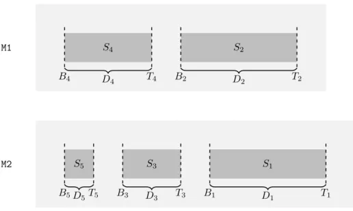
The optimum value is assumed to be known, and for sake of simplicity we will assume that OPT is equal to 1. (This can be assumed without loss of generality by normalization, i.e., dividing all of the job lengths by the optimal makespan.) Then we define five safe setsSi:= [Bi, Ti] with sizeDi:=Ti−Bi
fori= 1, . . . ,5 as follows (see also Figure 2):
1. B1:=s+ 1−randT1:=rs, thusD1= (s+ 1) (r−1), 2. B2:=s+ 1−srandT2:=r, thusD2= (s+ 1) (r−1),
3. B3:= 2s−2r−rs+ 2 and T3:=s(r−1), thus D3= 2r−3s+ 2rs−2, 4. B4:= 4s−2r−3rs+ 3 andT4:=r−1, thus D4= (3r−4) (s+ 1), 5. B5:= 6s−5r−4rs+ 6 andT5:= 10s−7r−7rs+ 9, thusD5= 4s−2r−
3rs+ 3.
These sets define time intervals, and they are called “safe” because if the load of the machine is in this interval, this enables a “smart” algorithm (as the one we introduce later) to finish the schedule by not violating the desired competitive ratio. In other words, from the point of view of an algorithm (which wishes to keep the competitive ratio low), we want to assign the actual job in a way that the increased load of some machine will be inside a safe set.
3 Properties
In this section we summarize some technical properties and estimations of the definitions and notions from the previous section, which are needed within the computations in the subsequent sections.
Lemma 1 r5(s)≥r2(s)fors≥q7.
Proof. r5(s)−r2(s) = s+12 − 12s+109s+7 = 9s2(9s+7)2−8s−13 ≥ 0, which is true since 9s2−8s−13≥0 holds if and only ifs≤4−
√133
9 ors≥ 4+
√133 9 =q7.
M2 M1
S5
D5 B5 T5
S3
D3
B3 T3
S1
D1
B1 T1
S4
D4
B4 T4
S2
D2
B2 T2
Figure 2: Safe sets.
Lemma 2 The following inequalities hold in the entire considered domain of the functionr, i.e., for all s∈[q6,√
3].
1. 3s+22s+2 < 43 <1.35< r(s)<minn
4s+3 3s+2,s+2s+1o
<2s+1s+1 <2.
2. 8s+76s+5 ≤r(s).
3. s+3s+2 <7s+55s+4 <s+12 ≤r(s)<6s+64s+5.
Proof. The rightmost part in Lemma 2.1, i.e. 2s+1s+1 < 2, holds trivially. All other claims in 2.1 and 2.2 but the ones which regardr5(s) are already proven in [11], thus we give only this unproved part here. Moreover, we give the proof for 2.3, whose claims were not considered before.
1. The leftmost lower bound holds as 3s+22s+2 < 43 is equivalent to 4(2s+ 2)− 3(3s+ 2) = 2−s > 0, and hence to s < 2. Further, it is easy to see that r(s) = s+12 > 1.35, since s > 1.7 in the domain of r5. Regarding the upper bound, 2s+1s+1 > s+2s+1 holds trivially sinces >1, thus it remains to show that r <minn
s+2 s+1,4s+33s+2o
. Note that 4s+33s+2 ≥ s+2s+1 for positives holds if and only if (4s+ 3)(s+ 1)−(s+ 2)(3s+ 2) =s2−s−1 ≥ 0, i.e., s≥ 1+
√5
2 ≈1.618. Therefore, for larges we need to show only that r < s+2s+1. We have s+12 −s+2s+1 <0, which holds sinces2−3≤0 is true.
2. For largeswe get that s+12 ≥ 8s+76s+5 holds if and only if (6s+ 5)(s+ 1)− 2(8s+ 7) = 6s2−5s−9≥0, i.e.,s≥ 5+
√241
12 ≈1.7103 =q6which is valid.
3. Regarding the leftmost inequality, 7s+55s+4 −s+3s+2 = 2(s−1)(s+1)
(s+2)(5s+4) >0 trivially holds. The next inequality holds since s+12 −7s+55s+4 = 5s2(5s+4)2−5s−6 >0 holds if s > 5+
√145
10 ≈ 1.7042 (and this value is smaller than q6). Regarding r(s)≥ s+12 , for large speeds the inequality holds trivially (with equality) and for regular speeds we have already seen the validity of the inequality in Lemma 1. Thus we are done with the lower bound; let us see the upper bound. For regular swe have 6s+64s+5 −12s+109s+7 = (9s+7)(4s+5)6s2−4s−8 ≥0, which is true, since 6s2−4s−8≥0 for s≤ 1−
√ 13
3 ands≥ 1+
√ 13
3 =q0 ≈1.535.
For larges we have 6s+64s+5 −s+12 = −4s2(4s+5)2+3s+7 = (s+1)(7−4s)
2(4s+5) ≥0, which is true sinces≤1.75.
In the next lemma we state some properties of the safe sets. Note that an alternative option to define the safe sets would be to require these properties below.
Lemma 3 1. D1=D2,
2. T1−T3=sandT2−T4= 1, 3. B3=B1−D1,
4. B4=B2−D3, 5. B5=B3−D4, 6. T5=B5+B4.
Proof. Proofs of the equalities in Lemma 3.1 to 3.4 were given in D´osa et al.
[11]. Since these proofs use nothing else than the definition of the safe sets, we do not repeat them. For proving 3.5 and 3.6 we use again the definitions of the boundaries.
5. B5+D4= (6s−5r−4rs+ 6) + (3r−4)(s+ 1) = 2s−2r−rs+ 2 =B3. 6. B5+B4= (6s−5r−4rs+ 6) + (4s−2r−3rs+ 3) = 10s−7r−7rs+ 9 =T5.
The next lemma proves that the safe sets are well defined in the sense that they are disjoint sets, and follow each other in the described order on the ma- chines.
Lemma 4 The following inequalities hold:
1. 0≤B4< T4< B2< T2,
2. 0< B5< T5≤B3< T3< B1< T1.
Proof. We note that in the paper D´osa et al. [11] we already introduced the first four safe sets (in the same way), with the same properties. In this paper we need the fifth safe set as well, moreover the claims of the lemma hold also for large values ofs, thus we need to give the proof of the lemma again. In the calculations we generally use Lemma 2, unless stated otherwise.
1. From r≤ 4s+33s+2 it follows that 0≤4s+ 3−3rs−2r =B4. From r > 43 and the definition we have that 0<(3r−4)(s+ 1) =D4=T4−B4. From r < s+2s+1 it follows 0<(s+ 1−sr)−(r−1) =B2−T4. Byr >1 we have that 0<(s+ 1)(r−1) =T2−B2.
2. We observe that for positive s the inequality 0 < 6s−5r−4rs+ 6 = B5 is equivalent to r(s) < 6s+64s+5, which holds. Lemma 3.6 states that T5−B5=B4, and thus usingB4>0 from Lemma 4.1 we haveT5−B5>0.
From r ≥ 8s+76s+5 it follows that 0 ≤ 5r−8s+ 6rs−7 = (2s−2r−rs+ 2)−(10s−7r−7rs+ 9) = B3−T5. From r > 3s+22s+2 it follows that 0 < 2r+ 2rs−3s−2 = D3 = T3−B3. From r < 2s+1s+1 it follows that 0 < (s+ 1−r)−s(r−1) = B1−T3. By r > 1 we have that 0<(s+ 1)(r−1) =D1=T1−B1.
We will need some further properties regarding the safe sets. These proper- ties make the later calculations easier.
Lemma 5 1. D1=D2>max{B2, D3}, 2. B2<1 andB1< s,
3. T3−T5≥B2, 4. B2≥B3, 5. T2≥B1, 6. D3> B4, 7. T4+D3> B2, 8. 2D1> s, 9. T4+D1>1, 10. T4+T2≥s.
Proof. We generally use Lemma 2 for the lower or upper bounds onr(s).
1. D1 = D2 holds directly by definition. For D2 > B2 we equivalently have D2−B2 = (s+ 1)(r−1)−(s+ 1−sr) = 2sr−2s−2 +r > 0, and hence r(2s+ 1) > 2s+ 2, which holds. Finally, from D2 −D3 = (rs+r−s−1)−(2r−3s+ 2rs−2) = −rs−r+ 2s+ 1 > 0 we get
2s+1
s+1 > r, which is true.
2. B2=s+ 1−sr <1, andB1=s+ 1−r < ssince 1< r.
3. We haveT3−T5−B2=s(r−1)−(10s−7r−7rs+ 9)−(s+ 1−sr) = 7r−12s+ 9rs−10≥0 if and only ifr≥12s+109s+7 . This is trivially true for anys≤q7, and true fors > q7by Lemma 1.
4. We have B2−B3 = (s+ 1−sr)−(2s−2r−rs+ 2) = 2r−s−1≥0 if and only ifr≥s+12 , which holds.
5. T2−B1=r−(s+ 1−r) = 2r−s−1≥0.
6. D3−B4= (2r−3s+ 2rs−2)−(4s−2r−3rs+ 3) = 4r−7s+ 5rs−5>0 if and only ifr > 7s+55s+4.
7. T4+D3−B2> B4+D3−B2= 0, by Lemmas 3.4 and 4.1.
8. 2D1−s= 2 (s+ 1) (r−1)−s= 2r−3s+ 2rs−2>0 holds if r > 3s+22s+2, which is true.
9. T4+D1−1 = (r−1) + (s+ 1) (r−1)−1 = 2r−s+rs−3>0 if and only ifr >s+3s+2.
10. T4+T2−s= (r−1) +r−s= 2r−s−1≥0 sincer≥ s+12 .
4 Algorithm FinalCases
First the loads are zero. The actual loads of the machines will be denoted as Lm (m= 1 or m= 2) just before assigning the next job. Thus, for example, ifL1denotes the actual load of the first machine, then after assigning a job to this machine, the new load will again be denoted byL1.
Here we define a subalgorithm, which works (and will be applied) only if the next job can be assigned to a machine whose increased load will be within some safe set. We call the algorithmFinalCases. We will say, for the sake of simplicity, that some step is executed if the condition of this step is satisfied and the actual job is assigned at this step. Otherwise we say that the step is onlyexamined. In other words, entering some step, it is examined whether the condition of the step is fulfilled or not. If yes, the step is executed. If not, the step is not executed. Moreover, for the sake of simplicity, if some step is not executed, we do not write “else if” in the description of the algorithm; if it turns out that the condition of some step is not satisfied, then the algorithm simply proceeds with examining the next step.
Theorem 6 Suppose that some of Steps 1 to 5 of Algorithm FinalCases is executed. Then all subsequent jobs are also scheduled by this algorithm, and the competitive ratio is not violated.
Algorithm 1:FinalCases
Data: current loadsL1, L2 for machinesM1,M2; index iof current jobxi
1 if L2+xi ∈S1then
L2:=L2+xi // assign job xi to M2 L1:=L1+PN
j=i+1xj // assign all subsequent jobs to M1
stop // no more jobs, terminate
2 if L1+xi ∈S2then
L1:=L1+xi // assign job xi to M1 L2:=L2+PN
j=i+1xj // assign all subsequent jobs to M2
stop // no more jobs, terminate
3 if L2+xi ∈S3 and L1< B2then
L2:=L2+xi // assign job xi to M2 whileL1+xi+1< B2 do
i:=i+ 1 // next job
L1:=L1+xi // assign job xi to M1
i:=i+ 1 // next job
goto Step 1
4 if L1+xi ∈S4 and L2< B3then
L1:=L1+xi // assign job xi to M1 whileL2+xi+1< B3 do
i:=i+ 1 // next job
L2:=L2+xi // assign job xi to M2
i:=i+ 1 // next job
if L2+xi ∈S1 orL1+xi∈S2 orL2+xi∈S3 then goto Step 1
whileL2+xi< B1 do
L2:=L2+xi // assign job xi to M2
i:=i+ 1 // next job
goto Step 1
5 if L2+xi ∈S5 and L1≤B4then
L2:=L2+xi // assign job xi to M2 whileL1+xi+1< B4 do
i:=i+ 1 // next job
L1:=L1+xi // assign job xi to M1
i:=i+ 1 // next job
if L2+xi∈S1 orL1+xi∈S2orL2+xi∈S3 orL1+xi∈S4 then goto Step 1
whileL2+xi< B1 do
L2:=L2+xi // assign job xi to M2
i:=i+ 1 // next job
goto Step 1
return // back to the main program, if used as subroutine
Proof.
1. Suppose that Step 1 is executed. Then the load L2 of the fast machine M2will be not more thanT1=rs, thus we do not violate the competitive ratio r by the fast machine. On the other hand, the final load of the fast machine is at leastB1=s+ 1−r, because we assigned jobxi toM2.
Applying SUM≤s+ 1, the final loadL1of the slow machineM1cannot be more thanr, sinceL1= SUM−L2≤(s+ 1)−(s+ 1−r) =r, which means that the competitive ratio is not violated by the slow machine either.
2. Now suppose that Step 2 is executed. The proof is almost the same as for Step 1. The load of M1does not exceedT2, so the competitive ratio is not violated by the slow machine. Moreover the final load of the slow machine isL1≥B2=s+ 1−sr, thusL2≤SUM−L1≤(s+ 1)−B2=sr=T1, and we are done.
3. Suppose that Step 3 is executed. After assigningxi toM2,B3≤L2≤T3
holds. Then we possibly assign several jobs to M1. We claim that the increased load of M1 cannot remain below B2. Indeed, assume that it stays below B2. ThenB2<1 from Lemma 5.2, and also Ts3 =r−1<1 from the rightmost estimation in Lemma 2.1. Hence the makespan would be strictly less than OPT = 1; a contradiction. Thus there must arrive a job that ends the loop, i.e. some jobxj withL1+xj ≥B2. At this point the algorithm goes back to Step 1. We claim that with this job xj the condition of Step 1 or Step 2 is satisfied, so the algorithm will assign all remaining jobs as explained above, and does not violate the competitive ratio.
Suppose that the condition of Step 2 is not satisfied, i.e.,L1+xj∈/S2. Together with the previously satisfied conditionL1+xj ≥B2, we deduce that L1+xj> T2, from which it follows thatxj > D2. We show that in this case the condition of Step 1 is already fulfilled. Indeed, for the lower bound we have L2+xj > B3+D2=B3+D1=B1 (where from left to right we applied the condition of Step 3, the definitions of D1 and D2, and Lemma 3.3), while for the upper bound we haveL2+xj≤T3+xj = s(r−1) +xj =sr−s+xj =T1−s+xj ≤T1 (where from left to right we applied the condition of Step 3, the definitions of T3 and T1, and the inequalityxj≤sdue to the fact that longer jobs would exceed OPT = 1 even on the fast machine). So we are entering Step 1 or Step 2.
4. Suppose that Step 4 is executed. After assigningxi toM1,B4≤L1≤T4 holds. Then we possibly assign several jobs to M2. We claim that the increased load of M2 cannot remain below B3. Indeed, assume that it stays belowB3. Then L1 ≤T4 =r−1 <1 from Lemma 2.1, moreover
B3
s < Bs1 <1, where we use Lemmas 4.2 and 5.2. Hence the makespan would be strictly less than OPT = 1; a contradiction. Thus there must arrive a job that ends the loop, i.e., some jobxj withL2+xj≥B3.
If L2+xj is in S1, or L1+xj is in S2, or L2+xj is in S3, we go back to Step 1. If Step 1 or Step 2 is executed, we are done. Otherwise the condition of Step 3 will be examined. We know that the condition L2+xj ∈S3 is fulfilled. Observe that the second condition of Step 3, i.e.
L1 ≤B2 also holds, sinceL1 ≤T4 still holds and we have T4 < B2 from Lemma 4.1. Thus Step 3 is executed, and we are done.
Now assume that none of the conditionsL2+xj ∈S1,L1+xj ∈S2, or L2+xj ∈ S3 is satisfied. Let us consider the size of the actual job, xj. Since L2+xj ≥ B3 (from the choice of xj), but L2+xj is not in S3, we deduce that L2+xj > T3. Hence together with L2 < B3 (also from the choice of xj) it follows that xj > D3. Then, using L1≥B4, we getL1+xj > B4+D3=B2 by Lemma 3.4. SinceL1+xj is not inS2, we also deduce that L1+xj > T2 holds. On the other hand, the actual load L1 of M1 is at mostT4. Thus xj > T2−L1 ≥T2−T4 = 1, where the equality comes from Lemma 3.2. Suppose that L2+xj > T1. Then xj > T1−T3 = s (by the first part of Lemma 3.2) would follow, which would violate the value of OPT, because even the faster machine M2can process this job within this makespan. Hence L2+xj ≤ T1. Together with the fact thatL2+xj ∈/ S1, we have thatL2+xj< B1. At this point xj is assigned toM2by the algorithm.
Now several subsequent jobs may be assigned to M2, while the load of M2remains below B1. But, similarly to the previous steps, there must arrive a further job xk that would exceed B1. Indeed, assume that no such jobs exists. Then L1 ≤T4 =r−1 <1 (by Lemma 2.1) and L2 ≤ B1 < s (by Lemma 5.2), so the makespan would stay below OPT = 1;
a contradiction. Thus the assignment of jobs to M2is stopped, and the algorithm goes back to Step 1.
We claim that one of Step 1 or Step 2 will be executed. If Step 1 is not executed, then L2+xk ∈/ S1 and L2+xk > B1 from the previous loop. Together,L2+xk> T1. SinceL2< B1, we obtainxk > T1−L2>
T1−B1=D1. Then we getL1+xk > B4+D1> B4+D3by Lemma 5.1, and B4+D3 =B2 by Lemma 3.4, hence L1+xk > B2. Assume that Step 2 is not executed either. ThenL1+xk ∈/ S2. HenceL1+xk > T2. From this is follows thatxk > T2−L1≥T2−T4= 1, becauseL1≤T4is still true and we haveT2−T4= 1 (from Lemma 3.2). Then there are two jobs, sayxk andxj, which are both bigger than 1, thus both have to be assigned to the fast machine in the optimal schedule. Therefore we have OPT>2s, and 2s >1 (from 2> s), which is a contradiction.
5. Finally, suppose that Step 5 is executed. We assign first the actual job to the machineM2and then we assign jobs to the machineM1untilL1+xi <
B4. Observe that L1 cannot remain below B4. Assume the opposite.
ThenL1≤B4< B2<1 by Lemma 5.2. Moreover,L2≤T5< B1< sby Lemma 2.1. Hence the makespan would be strictly less than OPT = 1; a contradiction. Thus there must arrive a job that ends the loop, i.e., some
jobxj withL1+xj≥B4.
If any of the four conditions L1 +xj ∈ S4, or L1 +xj ∈ S2, or L2+xj∈S3, orL2+xj ∈S1is satisfied, we go back to Step 1. Note that at this moment L1 < B4 < B2 andL2 ≤T5 < B3 (applying Lemma 4).
Hence it follows that some of Step 1 – Step 4 must be executed, and we are done. Therefore, suppose that none of the four conditions is satisfied.
Let us consider the size ofxj.
SinceL1+xj≥B4 (from the choice ofxj), but L1+xj is not inS4, we deduce thatL1+xj > T4. Hence together with L1 < B4 (also from the choice ofxj) it follows thatxj> D4. ThenL2+xj> B5+D4=B3, applyingL2≥B5 and Lemma 3.4. Since L2+xj is not inS3, it follows that L2+xj > T3. Together with L2 ≤T5, we get xj > T3−T5. Then L1+xj >(B2−T3+T5) + (T3−T5) =B2, applyingL1≥0≥B2−T3+T5
(Lemma 5.3). On the other hand, we know thatL1+xj is not inS2, thus it follows that L1+xj > T2. Consequently, using Lemma 3.2, we get y > T2−T4= 1.
We know thatL2+xj is not inS1. Suppose thatL2+xj> T1. Then xj > T1 −L2 > T1 −T3 = s would follow, applying Lemma 3.1, and L2≤T5< T3 by Lemma 4.1; a contradiction. Therefore at this point we assign xj to machine M2, and the increased load of M2 is strictly bigger thanT3and strictly smaller thanB1.
Now several subsequent jobs may be assigned to M2, while the load of M2 remains below B1. There must arrive a job, say xk, such that L2+xk≥B1. Indeed, assume that it stays belowB1. Since we know that L1≤T4, we conclude similarly to the proof of the previous point that this would lead to a makespan strictly less than 1 = OPT; a contradiction.
At this point the algorithm goes back to Step 1. We claim that either Step 1 or Step 2 will be executed. If Step 1 is not executed, thenL2+xk >
T1, sinceL2+xk ≥B1. This together withL2< B1implies thatxk> D1. Therefore we get L1+xk > D1 > B2, by Lemma 5.1. If Step 2 is not executed either, which means thatL1+xk∈/S2 and henceL1+xk > T2, thenxk > T2−L1≥T2−B4> T2−T4= 1, where we appliedL1< B4, B4< T4(by Lemma 4.1), andT2−T4= 1 (by Lemma 3.2).
Summarizing our analysis, we have two jobs,xj andxk, both greater than 1, thus both have to be assigned to the fast machine in the optimal schedule. Therefore we have OPT > 2s, and 2s >1 (from 2> s), which is a contradiction. Therefore Step 1 or Step 2 has to be executed and we are done.
We have seen that AlgorithmFinalCases solves the problem (does not vi- olate the competitive ratio) if some step of the algorithm is executed. The problem is that it may happen — although only rarely — that no step can be
executed because the condition of no step is satisfied. We must take care about these remaining cases. For this we define another algorithm in the next section.
We say that AlgorithmFinalCasesisexecutableif the condition of some step is satisfied. Summarizing our previous investigations, if AlgorithmFinalCases is executable, then doing so we obtain a schedule which does not violate the competitive ratio.
5 Algorithm InitialCases
In order to handle the case where AlgorithmFinalCasesis not executable, we now give the algorithmInitialCasesthat callsFinalCases as a subroutine.
Algorithm 2:InitialCases
1 L1:= 0, L2:= 0 // both machines are empty
i:= 1 // start with first job
whileL2+xi< B5 do
L2:=L2+xi // assign job xi to M2
i:=i+ 1 // next job
call AlgorithmFinalCases
2 L2:=L2+xi // assign job xi to M2
j:=i+ 1 // next job
whileL2+xj < B3do
L2:=L2+xj // assign job xj to M2
j:=j+ 1 // next job
call AlgorithmFinalCases
3 L1:=L1+xj // assign job xj to M1
k:=j+ 1 // next job
whileL2+xk < B3do
L2:=L2+xk // assign job xk to M2
k:=k+ 1 // next job
call AlgorithmFinalCases
4 L2:=L2+xk // assign job xk to M2
`:=k+ 1 // next job
whileL2+x`< B1 do
L2:=L2+x` // assign job x` to M2
`:=`+ 1 // next job
call AlgorithmFinalCases
For proving that AlgorithmInitialCasesisr-competitive in the considered interval, we still need one more claim as below.
Lemma 7 Suppose that machineM1is empty (i.e., L1= 0), and that the load L2 of machine M2is at most B5. If x is a job whose size satisfies x /∈S2 and L2+x /∈S1, then x≤T3−B5.
Proof.Assume thatx > T3−B5. SinceT3−B5≥B2(by Lemma 5.3), it follows thatx > B2. Recall that there is no job assigned toM1so far. Sincex /∈S2, we obtainx > T2≥B1(where the last estimation was shown in Lemma 5.5). From x > B1it then follows thatL2+x > L2+B1≥B1. Together withL2+x /∈S1, we deduce thatL2+x > T1. Hencex > T1−L2≥T1−B5> T1−T3=s=s·OPT (by Lemma 4.2 and Lemma 3.2). This is a contradiction, since no job can be bigger thans·OPT.
After this, we state the next theorem.
Theorem 8 Algorithm InitialCasesisr-competitive for anyq6≤s≤√ 3.
Proof.
1. If Algorithm FinalCases is called in Step 1 and there all jobs are as- signed to machines (in Step 1 and Step 2 of AlgorithmFinalCases), then FinalCases terminates and all jobs are within the safe sets, so the com- petitive ratio ofris not exceeded.
At the end of Step 1, let us denote the actual job by xi. It holds that L2+xi ≥ B5, and before xi came, L2 was below B5. Algorithm FinalCases was called at the end of Step 1, but none of the conditions of the five Steps 1–5 in Algorithm FinalCases was actually true (i.e., FinalCases was not executable). In particular, Step 5 of FinalCases was not executed. SinceL1= 0 (machineM1is empty), andB4>0 (from Lemma 4.1), it thus follows that L2+xi > T5. Together with L2 < B5
it follows from Lemma 3.6 that xi > T5−B5 = B4. Note that at this point still there is no job assigned to M1. Since xi is not assigned to M1 (asFinalCaseswas not executable), in particular, Step 4 of FinalCases is not executable. SinceL2 < B5< B3 (from Lemma 4.2), it means that L1+xi∈/ S4. Fromxi > B4(see above) it then follows thatxi > T4.
Suppose thatxi > B3 holds (from which we derive a contradiction).
Then it follows that xi > T3−B5, because otherwise, if xi ≤ T3−B5, then T3 ≥ xi+B5 > xi +L2 > xi > B3, hence L2+xi ∈ S3. Since L1 = 0 < B2 (from Lemma 4.1), it follows that Step 3 of Algorithm FinalCases would be executed; a contradiction. Hence xi > T3−B5. Note that all assumptions of Lemma 7 are satisfied. Hencex1≤T3−B5; a contradiction. Thereforexi≤B3.
Thus we conclude from the previous two paragraphs that T4 < xi <
B3.
Let us investigate how big the actual load of M2would be, if xi was assigned to this machine; that is, we want to estimate L2+xi. We are going to show thatT5< L2+xi< B3, by excluding all other possibilities.
To prove the lower bound, note that since the algorithm terminated the while-loop, we haveL2< B5 and L2+xi ≥B5. As we argued above, we know thatL2+xi∈/S5, hence we haveL2+xi> T5. To prove the upper bound, we need to exclude two more cases (see also Figure 2).
(a) Suppose that L2 +xi ∈ S3 = [B3, T3]. Since L1 = 0 ≤ B2 (by Lemma 4.1), Step 3 of AlgorithmFinalCases would have been exe- cuted; a contradiction. ThusL2+xi ∈/ [B3, T3].
(b) Suppose that L2+xi > T3. Then xi > T3−L2 > T3−B5 (since L2 < B5, see above). Note that all assumptions of Lemma 7 are satisfied. Hencex1≤T3−B5; a contradiction. Thus L2+xi≤T3. Consequently,T5< L2+xi< B3.
2. We enter Step 2. We assignxi to M2. From the analysis above we know that the loadL2after this assignment is aboveT5 and belowB3.
Then several jobs may come, and they are assigned to machine M2, while the loadL2of M2remains below B3. This termination point of the while-loop will come for sure: otherwise we would have an empty machine M1, and the total load of all jobs, all on machineM2, would be still below B3. SinceB3< B1< s=s·OPT (by Lemma 5.2 and Lemma 4.2), this contradicts the assumption that the optimum value is OPT.
Letxj denote the job upon terminating the while-loop. Now we call Algorithm FinalCases with this index j. Assume FinalCases is not executable (otherwise we are done). It holds thatL2< B3andL2+xj ≥ B3. Furthermore,L1= 0≤B2 (by Lemma 4.1), but Step 3 of Algorithm FinalCaseswas not executed, thusL2+xj ∈/S3. Consequently,L2+xj >
T3, and thusxj > D3. By Lemma 5.6 we have D3> B4. Since no job is assigned to M1, and Step 4 of FinalCases was not executable, moreover L2≤B3, we have thatL1+xj =xj ∈/ S4. Fromxj > D3> B4we deduce xj> T4.
The assumption of xj ≥ B2 will lead to a contradiction as follows.
Since Step 2 of FinalCases was not executable, it holds thatL1+xj = xj ∈/ S2, hencexj > T2. In Lemma 5.5 we proved thatT2 > B1, hence xj > B1. Since also Step 1 of FinalCases was not executable, it holds thatL2+xj ∈/ S1. Fromxj > B1we thus deduce thatL2+xj > T1. Thus we estimate xj > T1−L2 > T1−T3 =s, where the second estimation usesL2 < B3 < T3 and the last inequality is due to Lemma 3.2. Hence xj > s=s·OPT, so job xj would be too large for an optimum value of OPT.
Summing up, we conclude thatT4< xj< B2 holds.
3. In Step 3 we assignxj toM1, and since this is the only job which has been assigned toM1 ever, the loadL1of M1is betweenT4andB2.
Then again, several jobs may come, and they are assigned to machine M2, while the loadL2 of M2remains belowB3. This termination point of the while-loop will come for sure: otherwise we would have machine M1 with a load lower than B2 < 1 = OPT by Lemma 5.2, and the load of L2 is belowB3< B1< s=s·OPT by Lemma 5.2. This contradicts the assumption that the optimum value is OPT.
Letxk denote the job upon terminating the while-loop. Now we call AlgorithmFinalCaseswith this indexk. Assume thatFinalCasesis not executable (otherwise we are done). In particular, Step 3 of FinalCases was not executable, and since L1 ≤ B2, it follows that L2+xk ∈/ S3. Taking into account that L2 < B3 and L2+xk ≥ B3, it follows that L2+xk> T3, hencexk> D3.
From Lemma 5.7 it follows thatxj+xk−B2> T4+D3−B2>0, thus xj+xk > B2. Since Step 2 of FinalCaseswas not executable, it means that L1+xk =xj+xk ∈/ S2, hence xj+xk > T2. SinceL1 =xj ≤B2, we havexk > D2=D1(by the definition ofD1 andD2).
Assume that L2+xk ≥ B1. Since Step 1 of FinalCases was not executed, it would follow that L2+xk ≥T1. Thus taking into account that L2 < B3, we obtain the estimation xk ≥ T1−L2 > T1−B3 >
T1−T3=s=s·OPT (by Lemma 4.2 and Lemma 3.2), which contradicts the optimality of value OPT. ThusL2+xk< B1.
4. We start Step 4 with assigningxk toM2. Then the new loadL2is between T3andB1.
Then for the last time, several jobs may come, and they are assigned to machine M2, as long as the load L2 of M2 remains below B1. The termination point of the while-loop will come for sure: otherwise we would have a machineM1with a load lower thanB2<1 = OPT (by Lemma 5.2), and the load of L2 is below B1 < s = s·OPT by Lemma 5.8. This contradicts the assumption that the optimum value is OPT.
Letx` denote the job upon terminating the while-loop. We will show that nowFinalCasesis executable, thus we are done. Assume the oppo- site: FinalCases is not executable.
At this point we haveL2< B1 andL2+x`≥B1. SinceFinalCases is not executable, in particular, Step 1 ofFinalCaseswas not executable, meaningL2+x`∈/S1. Hence L2+x`> T1, thusx`> D1.
Using xj > T4 from Step 2 above, we can estimate xj+x` > T4+ D1 > D1 > B2 using Lemmas 4.1 and 3.1. Since at this point only xj
is assigned to M1, and Step 2 of FinalCases is not executable, that is L1+x`=xj+x`∈/S2, it also holds thatxj+x`> T2.
We summarize: xi, xj> T4,xk, x`> D2=D1, moreoverxj+xk> T2 andxj+x`> T2.
Note thatxk+x`>2D1> s=s·OPT (by Lemma 5.8). So it follows that xk and x` must be assigned to different machines in any optimum schedule, because even the faster machine M2 cannot handle both jobs within a makespan of OPT.
First, consider an optimum schedule wherexk is assigned to the slower machineM1andx` is assigned to the faster machineM2. Assume that xi
is also assigned to M1. Then we can estimate the load of this machine:
![Figure 1: Known and new upper and lower bounds from Epstein [15], Ng et al.](https://thumb-eu.123doks.com/thumbv2/9dokorg/1074169.71892/6.918.211.713.192.491/figure-known-new-upper-lower-bounds-epstein-ng.webp)