Prediction of biological activity using heterogeneous information sources
PhD thesis
Ádám Arany
Semmelweis University
Doctoral School of Pharmaceutical Sciences
Supervisor: Dr. Péter Mátyus, DSc
Official reviewers: Dr. Gábor Horváth, Ph.D.
Dr. Tóthfalusi László, Ph.D.
Head of the Final Examination Commitee: Dr. Imre Klebovich, DSc Members of the Final Examination Commitee: Dr. László Őrfi, Ph.D.
Dr. Tamás Paál, CSc Budapest
2016
1 Table of Contents
2 Abbreviations ... 4
3 Introduction ... 7
3.1 Pharmaceutical Industry Background ... 8
3.2 Overview of Virtual Screening ... 14
3.3 Overview of Data fusion ... 17
3.4 Network pharmacology ... 21
3.5 Evaluating the performance of virtual screening ... 28
3.6 Probabilistic graphical models in the Bayesian statistical framework ... 38
3.7 Bayesian framework ... 38
3.8 Bayesian networks ... 40
3.9 Bayesian Multilevel Analysis of Relevance ... 42
3.10 Machine Learning methods ... 43
3.11 Linear methods for quantitative prediction ... 43
3.12 Basics of kernel methods... 47
3.13 Data fusion with kernel methods ... 49
3.14 One-class Support Vector Machines ... 51
3.15 Semi-supervised and Positive and Unlabelled Learning ... 53
3.16 Generalization error and cross validation ... 55
3.17 Macau: Bayesian Multi-relational Factorization ... 56
4 Objectives ... 60
5 Methods ... 61
5.1 Information sources ... 61
5.2 Redundancy and complementarity of the information sources ... 69
5.3 Evaluation framework for the fusion methods... 69
5.4 Drug-Indication reference set ... 70
5.5 Application for Parkinson's disease therapy ... 71
5.6 Evaluation of Macau ... 74
5.7 Analysis of the methotrexate pharmacokinetics ... 76
5.7.1 Patient data ... 79
5.7.2 Bayesian multilevel relevance analysis ... 79
6 Results ... 81
6.1 Fusion of heterogeneous information sources for the prediction of the biological effect of small-molecular drugs ... 81
6.2 Application of the Kernel Fusion Repositioning method for finding Parkinson's disease related drugs ... 89
6.3 Predicting multiple activities simultaneously improves the accuracy ... 97
6.4 Comparison of BN-BMLA results to frequentist statistics in the task of associated variance detection for interpersonal methotrexate pharmacokinetics variability ... 99
7 Discussion ... 102
7.1 Fusion of heterogeneous information sources for the prediction of biological activity ... 102
7.2 Application of the Kernel Fusion Repositioning framework to find Parkinson's disease related drugs ... 103
7.3 Prediction of multiple targets simultaneously ... 104
7.4 Advantages of Bayesian methods ... 104
8 Conclusions ... 106
9 Summary ... 108
10 Összefoglalás ... 109
References ... 110
List of own publications ... 118 Acknowledgements ... 119
2 Abbreviations
ADME Absorption, Distribution, Metabolism, Excretion
ATC Anatomical Therapeutic Chemical classification system
AUC Area Under the Curve
BEDROC Boltzmann-Enhanced Discrimination of ROC
BN-BMLA Bayesian Network based Bayesian Multilevel Analysis BPMF Bayesian Probabilistic Matrix Factorization
CNS Central Nervous System
COM Composition of Matter (patent)
CROC Concentrated ROC
CSEA Compound Set Enrichment Analysis
DAG Directed Acyclic Graph
EF Enrichment Factor
FDA Food and Drug Administration
FN False Negative
FP False Positive
GO Gene Ontology
GSEA Gene Set Enrichment Analysis
HCI High Content Imaging
HDACi Histone deacetylase inhibitor
HLGT High Level Group Term (MedDRA)
HLT High Level Term (MedDRA)
HPO Human Phenotype Ontology
HTS High Throughput Screening
IND Investigational New Drug
INN International Nonproprietary Name
IR Infrared (spectroscopy)
ISS IntraSet Similarity
KFR Kernel Fusion Repositioning
LLT Lowest Level Term (MedDRA)
MAF Minor Allele Frequency
MAO-B Monoamine Oxidase B
MCMC Markov-Chain Monte Carlo
MeSH Medical Subject Headings
MKL Multiple Kernel Learning
MOU Method of Use (Patent)
NME New Molecular Entity
NMR Nuclear Magnetic Resonance
OLS Ordinary Least Squares
PCA Principal Component Analysis PCR Principal Component Regression PGM Probabilistic Graphical Model PLS Partial Least Squares regression
PPARγ Peroxisome proliferator-activated receptor gamma PPI Protein-Protein Interaction (network)
PT Preferred Term (MedDRA)
PU Positive and Unlabelled (learning)
QSAR Quantitative Structure-Activity Relationship
RBF Radial Basis Function (kernel)
ROC Receiver Operating Characteristic curve
ROS Reactive Oxygen Species
SAR Structure-Activity Relationship SEA Similarity Ensemble Approach SMARTS Smiles Arbitrary Target Specification SNP Single Nucleotide Polymorphism
SNRI Serotonin-Norepinephrine Reuptake Inhibitor
SOC System Organ Class (MedDRA)
SSRI Selective Serotonin Reuptake Inhibitor SUI Stress Urinary Incontinence
TN True Negative
TP True Positive
UAS Universal Average Similarity UMLS Unified Medical Language System
3 Introduction
As the productivity of the pharmaceutical research and development is lagging behind the sharply increasing costs, the pharmaceutical industry is continuously searching for new approaches in drug discovery. These problems are aggravated also by the price pressure caused by expiring patents, and the ever complicated regulatory procedures. In my doctoral research I developed and applied methods related to two topics, which revolutionized the pharmaceutical industry to ameliorate the effect of the dropping effectiveness of the research and development pipeline: drug repositioning and personalized medicine (Figure 1).
Figure 1 – The investigated topics and their common characteristics.
Drug repositioning or repurposing is a cost-effective and risk-reducing straightforward strategy, which aims at reusing already approved drugs in new therapeutic indications.
From the machine learning perspective the main distinctive feature of drug repositioning
Figure 2 - Topics related to drug repositioning and their relations.
compared to de novo drug discovery is the availability of a wide range of information sources. While conducting the research my primary goal was to develop computational methods to harness these information sources in drug repositioning (see Figure 2). As a first step I created a benchmark dataset containing six different information sources (three chemical structure descriptors, two side effect based descriptors and a target profile), and a drug-indication gold standard set. The goal of my first computational experiment was to compare a novel data fusion methodology, called Kernel Fusion Repositioning (KFR), with a baseline method. My contribution primarily concerned the design and implementation of the KFR framework as well as the application of the KFR framework on the problem of repositioning for Parkinson’s disease. As one of the authors of a novel multi-target prediction method I also applied this method to the repositioning benchmark, and analysed the effect of multi-target learning on accuracy.
My second topic was related to personalized medication, which facilitates the optimal therapy for the patient and is also favourable for the researcher interested in drug development. Predicting the patient-by-patient variability of the pharmacokinetics can help the investigator adjust the doses in a personalized way in order to maximize efficacy and minimize side effects and toxicity. I participated in researching the interpersonal variability of methotrexate pharmacokinetics at high dose levels, developed new clinical descriptors bridging patient and treatment levels, and investigated their usage by applying a novel Bayesian multivariate statistical technique to identify predictive genetic variants.
Moreover, I compared the results against already existing ones based on frequentist statistics.
3.1 Pharmaceutical Industry Background
The past two decades in the pharmaceutical industry have been characterized by decreasing research and development productivity, high attrition rate and high volatility of output. Nowadays a dramatic shift has taken place in the field, including more pre- competition time collaborations, public-private partnerships, and an extremely high number of mergers and acquisitions [1]. The cost of developing a new drug is steadily increasing, while the yearly number of accepted New Molecular Entities (NMEs) is constant or even decreasing regarding only the small molecular drugs. These trends
is deteriorating and the complexity of developing a new drug and the time needed for it is growing significantly [2]. One of the several possible causes of this increased complexity is the stricter regulation environment well illustrated by the increasing number of guidelines [3].
The concentration of research and development efforts in therapeutic areas with larger patient population and higher risk, like chronic and potentially lethal diseases can be observed. A significant exception is the case of rare or orphan diseases, where governmental regulation, like the US Orphan Drug Act and the Regulation (EC) 141/2000 in the EU influence the market [2].
A somewhat radical suggestion to change the patent and the regulatory system has been also discussed in the literature [3]. It is generally accepted that the pharmaceutical industry heavily uses the patent system and employs defensive strategies which can be counterproductive and can further decrease productivity through feedback loops. In the recent years the fear of sharing information seems to ease, but it is still quite prominent.
Another way to move the system to a more cooperative mode of operation is to encourage the cooperation between the academia and the industry in a way that protects the academic focus on the long-term goals and high risk innovation.
The history of modern pharmaceutical industry was started by the large scale manufacturing of penicillin. At that time regulation was less strict, only safety studies were required for approval. Essential changes have taken place after the Contergan case, which have led to the introduction of the drug law, the ”Arzneimittelgesetz” in Germany, and with a bit logical jump to the Hatch-Waxman act in the USA [4, 5].
In the United States a notable step toward the current regulatory system was the enactment of the Drug Price Competition and Patent Term Restoration Act, often referred to as the Hatch-Waxman Act in 1984. It is useful to shortly examine this law, because it has indirect effects to the pharmaceutical development in the entire world. The main goal of the act is to facilitate generic development and price competition. It is achieved firstly by declaring the sufficiency of bioequivalence studies for generic product approval. A generic company can now enter the market by showing with bioavailability studies that their product is equivalent to the original medicine. The originator always has a 5 year data exclusivity period from approval. During this time the original clinical trials cannot
be used in the registration process of the generic competitor product. As a kind of compensation to stimulate research, patent term restoration has been introduced, which means that half of the time spent between the patent submission and the beginning of the marketing period, but maximum 5 years, can be added to the market exclusivity period of the originator. The whole exclusivity period cannot be longer than 14 years.
In the pharmaceutical industry remarkable volatility of the approval rate appeared in the mid-90s. However a dramatic market entry-exit volatility already existed in the 80s, increased explosively in the 90s and the first decade of the 2000s due to mergers and acquisitions. These trends led to an increasing number of managed NME per organisation.
This concentration of patented products led to the birth of a new type of market player, the 'Big Pharma'. Many of these companies do not carry out direct research and development activity or only in limited number, but obtaining NMEs by acquisitions of small companies instead [1].
Historically the time needed for developing a drug from the first screen was 10-15 years, but now this pipeline length is increasing. A target discovery phase, where the main question is the relevance of a target in a particular disease, usually precedes the de novo development, but this is out of the scope of the present work. The identification of the compounds starts with in-vitro or in-silico screening, usually High Throughput Screening (HTS) or virtual screening, where the goal is to search for hits, molecules with high probability of target binding. The preclinical development phase in a broader sense includes the classical chemical development steps such as hit-to-lead transition, lead optimization (changing substitution) and synthesis scale up. Strictly speaking the preclinical studies are experiments carried out to prove that the compound is safe to start human studies. These experiments include metabolic stability assays, toxicology studies and limited efficacy studies on model organisms. Before an experimental compound can be tested on human subjects, it need to be registered at the authority as an investigational new drug (IND). The Human Clinical Trials are divided into phases. During the Phase I studies, the main goal is to characterize the safety profile of the compound: determine the maximal safe dose and the absorption, distribution, metabolism, excretion profile (ADME) using increasing doses. These trials are usually carried out with the involvement of 100 or less healthy volunteers. In special indications like cancer a more frequent adverse
the safety study, usually called Phase I/II study, involves patients and the determination of a small sample based estimate of the efficacy is also possible. In Phase II the goal is the determination of human therapeutic efficacy with participation of limited number, typically hundreds, of patients. This phase is sometimes divided into sub-phases, like II/A and II/B. The classical setup is a double-blind placebo controlled setting, but it is not always applicable. If an already established therapy exists for the disease, for ethical reasons the control is frequently that existing therapy, and the new compound is given on its own or as an add-on to the classical therapy. The Phase III trial is an extension of the Phase II to 5-8000 patients as a multicentre trial. The successful closure of the Phase III is an essential prerequisite for a regulatory approval. If an already approved drug is tested and found effective in a new indication, a regulatory submission is made for label expansion. This type of submission has considerable interest concerning this work. The process is not finished at the point of approval. The final phase of the compound's lifecycle is the postmarketing phase, or Phase IV, which is about the continuous monitoring of safety also known as pharmacovigilance [6]. The manufacturers together with the medical doctors and the patients continuously monitor adverse events. The continuous data acquisition and interim analysis is pervasive during the whole pipeline both for ethical and financial reasons [7]. In the European Union the 'Community code relating to medicinal products for human use' (Directive 2001/83/EC) outlines the main regulatory background.
Regarding the detailed structure of the unsuccessful cases in the 2011-2012 interval, the main cause of failure in Phase II and III Clinical Trials was the lack of efficacy (56%), followed by safety issues (28%) [8]. The most expensive failure is which happens during Phase III; therefore early termination of the probably unsuccessful projects is an interest of the company. This fail-fast approach can be an explanation for the increase of attrition rate in Phase II and the decrease of failure rate in Phase III. It is worth pointing out that the rate of safety failures increased significantly during Phase III, which can serve as a motivation for this work, because suggesting approved and safe drugs for new indications can decrease the number of safety failures [8]. An analysis from 2014 suggests that the research and development output of the industry is still not satisfactory [9].
Drug repositioning or repurposing, i.e. searching for an innovative therapeutic application for an old drug, is a cost-effective and risk-reducing strategy in pharmaceutical research
and development. For an existing compound already approved as a drug in some indications toxicity and pharmacokinetics parameters like ADME profile are available at least in some dosage and for some routes of administration [10]. The already developed manufacturing process or synthesis scale-up can also lower the costs.
The classical case of drug repositioning is when a late failed candidate repositioned to a new indication. The serendipitous observation which led to the repositioning of thalidomide is a good example for this classical route [4]. During a four year period thalidomide with the trade name Contergan was originally marketed as a sedative especially for pregnant women. After its withdrawal due to its serious teratogenic side effects a clinical observation led to its application in erythema nodosum leprosum.
Similarly, the phosphodiesterase-5 inhibitor sildenafil was in clinical phase for angina, but it failed to favourably influence the clinical outcome. However, its side effect later led to its approval against erectile dysfunction with a trade name Viagra [4].
The case of duloxetine is near to what is called a branching development strategy. Eli Lilly and Co. originally developed the compound as a serotonin-norepinephrine reuptake inhibitor (SNRI) antidepressant later marketed in this indication with the trade name Cymbalta. During its development process, based on a mechanistic observation stress urinary incontinence (SUI) as a new indication was suggested [4, 11]. This repositioning was successful, and duloxetine got approved for SUI with the trade name Yentreve.
We can regard drug repositioning as a lifecycle management, which led to the new trend of early repositioning [12]. The available information during the development process has a funnel structure. The information from the early stages is available for a large set of compounds, it is general, and it can be used independently of the indication, but it is a weak predictor of the clinical outcome. As we proceed, the gathered information will be closer to the clinical endpoint, but its specificity for indications will be higher and higher [12].
In fact the most successful repositioned drugs are based on serendipity, despite the several existing systematic approaches [13, 14]. The evidences show that there is need for technological intellectual property beside of expert knowledge for a repositioning biotech to be successful [13]. An important aspect to understand the difficulty of drug repositioning in a classical pharma company is the management mentality against funding
already failed projects. Another difficulty is that the strategic focus indications are specific for a given company, so if we reposition a proprietary molecule it is highly probable that there is no clinical expertise available in this new indication [13].
Two important types of patent need to be discussed here [4, 13]. The strongest one in the sense of protection is the composition of matter (COM) patent, which claims the chemical structure of the compound and grants 20 years of protection from the patent application.
A company needs to protect the compound in development at least before registering it as an IND, so at least half of the time spent in the clinical phases is lost from the market exclusivity period. Therefore, starting a new clinical development phase after a late failure is a risky decision. If a compound fails in Phase III, the company loses too much time to start a new trial: a favourable alternative can be a branched development program [12, 13]. This extended profiling or early repositioning of a drug candidate can facilitate the deeper understanding of the safety and side effect profile of the compound [12, 13].
The other important type of patent in the field of drug repositioning is the method of use (MOU), which claims that the compound can be used to treat a disease. Because the original COM patent usually covers a lot of indications, constructing a MOU patent can be very difficult. Another way to get a new COM patent is the combination of active substances, which forms the base strategy for some of the repositioning biotech companies [4]. In case of the orphan diseases, as already mentioned, an extra protection is granted by the law [13].
Another route to improve the productivity of the pharmaceutical pipeline is the stratification of the patient population. In a more homogeneous population, where a well- defined disease state is present, the lack of efficacy type failures can be reduced [15]. In several cases diseases known in the past as a uniform group actually have several different aetiologies. An excellent example for this is the case of targeted tumour therapies, but the disease heterogeneity is observable in several other therapeutic areas like neurodegenerative diseases or immunological conditions as well [15-17]. This effect can result in apparent inefficacies in clinical trials, as we try to target an ill-defined disease instead of the aetiology.
Drug development for rare or orphan diseases faces with the same complication as stratified patient population: the number of patients can be very low. If we can identify a
common molecular mechanism between diseases, we develop a drug to that mechanism.
Another route is drug repositioning: if we can find a drug already registered in a classical indication which can be applied in the rare case, we can use it as a candidate.
Another important factor is the pharmacokinetics related heterogeneity of the subjects.
Genetic polymorphisms in metabolizing enzymes and transporters can result in significant differences of drug metabolism and therefore can cause a lack of efficacy and toxicity problems.
3.2 Overview of Virtual Screening
To find novel pharmaceutically active compounds with appropriate properties and a patentable new structure sometimes millions of candidates should be analysed. If we can reduce the number of compounds we need to test in an HTS setting, we can reduce the cost of the early phase of the screening program dramatically. Moreover, sometimes the in-house dataset does not provide enough chemical diversity, therefore we plan to use candidates from external sources or to synthetize new chemistry. In this case, identifying a subset of compounds with the highest probability of activity before candidate acquisition or synthesis would result in even higher benefits.
These computational screening methods can be divided into two main classes, target- based methods and ligand-based methods. In the first case, when the structure of the target is known, this information together with the possibly available structure of known target- ligand complexes can be exploited to guide the search for new active compounds. Most often these target structures are available in the form of X-ray crystallography or NMR measurements. In the other case, ligand-based methods only use the structural information of known active and known inactive compounds and attempts to identify the key elements of the structure-activity relationship (SAR) using statistical techniques. In this work we are particularly interested in ligand-based techniques. The most important categories of these methods are similarity searching, classification and quantitative structure-activity relationship (QSAR) modelling. One of the obvious differences of these methods is that they provide ordinal, categorical and numerical predictions respectively.
In its simplest form similarity searching is a basic tool requiring only a single reference compound, and returning a list of neighbours from the database, ordered from the most
similar to the least similar one. Assuming that the similar property principle holds – two compounds with high global similarity have high probability to share the same biological activity – the biologically active compounds will be enriched on the top of the ranking.
The similar property principle is based on the assumption of a smooth structure-activity relationship in the chemical space [18, 19]. While pharmacophore analysis and QSAR based methods focus on local features of the chemical compound, the similar property principle suggests an inherently global viewpoint [18]. This global similarity viewpoint assumes a continuous relation between chemical structure and activity: small changes in molecular structure cause small changes in activity. Therefore its validity is limited by activity cliffs, which can be caused for example by rigid structural elements in the binding site of the target.
A good example for this sudden change of activity in the chemical space is the so called
„magic methyl effect”, where introducing a single methyl group to a compound can result in several fold changes in activity. It is hardly surprising that using purely statistical approaches may lead to the misclassification of some samples near to an activity cliff as outlier. Without background knowledge, a sudden change of the activity caused by an activity cliff and a measurement error cannot be distinguished. In spite of the steric limits and well defined pharmacophoric interactions, the structural plasticity of the binding site makes it possible that in practice the biological activity is a smooth function of the chemical similarity in some regions of the chemical space. These factors also explain the strong dependence of the predictive performance on the target protein and on the reference compounds in question [18, 20]. Moreover, the performance depends on the molecular description method used, and on the different binding modes of similar ligands.
The above mentioned properties of the chemical space confirm the necessity of data fusion to exploit the advantages of the different methods and reference structures.
To define similarities between compounds we need an appropriate mathematical representation of a molecular structure, on which we can apply a function defining the similarity metric we want to use. The most straightforward approach to represent a chemical compound which meets the requirements described above is to assign a vector of numbers to it. This vector is usually called molecular descriptor. Every position in the vector - either binary, categorical or continuous – encodes a feature of the compound. If the position encodes the occurrence of a substructure, the descriptor is also called
molecular fingerprint. The substructure encoded can be two dimensional or three dimensional. In theory 3D fingerprints would contain more information than 2D ones, but in practice experience shows that most of the time the models based on the former show better predictive performance. A possible cause of this is the uncertainty of the relevant conformation used for calculating the 3D descriptor. Since the 2D fingerprint can be calculated directly from the graph structure of the compound, it is more robust.
Most of the time the number of possible substructures is enormous, while the vast majority of them is missing from a given compound. To handle this situation a function with low collision probability – the hash function - is used to map all possible substructures to a lower dimensional vector. Another solution is folding, when positions in a vector are merged and the new position is set to be active if any of its ancestor was active.
Another problem is that similarity is subjective; as Maggiora et al. said „similarity like beauty is more or less in the eye of the beholder” [20]. Or as a machine learning practitioner would say, the selection of the similarity metric should depend on the goal we would like to reach with modelling; that is, it should be determined in a supervised way.
There is a significant difference between classical similarity searching and machine learning methods. This difference is the weighting. Computing similarities between actives and candidates and then applying a predefined similarity threshold does not work, as the optimal threshold depends on the reference compound [20]. When machine learning approaches are used the similarity that we compute will depend on those substructures which are relevant for the binding process, and the possible many irrelevant common substructures will have a low weight.
The most popular similarity metric used on binary fingerprints is the Tanimoto or Jaccard metric. Its most popular chemoinformatics definition in its vectorial form is the following:
or written with sets (Jaccard definition):
The Tanimoto similarity is only used on binary vectors in this work. A possible generalization of the Jaccard similarity to non-binary vectors exists for multisets, sets where the number of occurrence of a substructure is also taken into account:
There are several application areas for molecular similarities, probably the most famous ones are the already mentioned database searching and activity prediction. Molecular similarity also has its application in assessing intellectual property positions and diversity based library enrichment [20]. In these two latter applications our goal is to maximize dissimilarity.
3.3 Overview of Data fusion
Molecules have many different types of measurable or computable characteristics from as simple ones as elemental composition, 2D structure, 3D structure, and physicochemical properties to as complex ones as phenotypic effects in a biological system, which makes the available data very heterogeneous. This heterogeneity is especially high in case of drug repositioning where we can work with much better characterized compounds. The relative importance of these characteristics depends on the scientific question we want to answer. The combination of this type of heterogeneous data should be problem specific, which imposes a significant mathematical challenge. Even in the prediction of drug action, different types of features and different inter-molecular similarity metrics can be predictive for different targets. This type of „no free lunch” characteristic, which is inherent in nature, makes the task even more challenging. The no free lunch behaviour is well known, and mathematically proven in the case of machine learning models [21].
What we call data fusion has always been organic chemists' general practice in a smaller scale. Let us consider a structure elucidation process based on infrared (IR) spectra, mass spectrometry and different multidimensional nuclear magnetic resonance (NMR) experiments. These spectroscopic measurements provide information about the different
aspects of the unknown compound. IR informs us about functional groups with characteristic bands, mass spectrometry about exact molecular mass, and optionally fragmentation data. On the other hand, NMR provides a wide range of information from local environments of protons, carbon, nitrogen, oxygen, phosphorus, fluorine atoms among others, and pairwise bond count distances, or even distances in the three dimensional space. All of these fragments of information, even if some of them are highly redundant, can be used to deduce the structure of the unknown compound with high confidence. In the modern era of big data our need to synthetize information and knowledge is still present, we just need computers to understand the relations in this enormous volume of data.
In chemoinformatics, it is very popular to fuse rankings or scores derived by different methods based on different information sources. In case of the rank fusion, we order the possible candidates (here compounds) and fuse this ranked list to a consensus ranking.
This process can be interpreted as a special case of quantile normalization, a statistical technique often used in expression microarray data analysis [22, 23].
In an earlier chemical application of data fusion basic min-rank, max-rank or sum-rank rules were evaluated on the individual rankings [24]. These rules simply calculate the minimum, maximum or average of the given compound's rank in the different lists, and reorder them using this new derived score. The sum-rank rule is commonly referred to as Borda protocol in information retrieval, which name is used in this work. It is originally an election method named after the French mathematician Jean-Charles de Borda. When applying this method, each voter creates a full preference list of the candidates, and scores them inversely to their preference: gives N point to the first candidate, N-1 to the second, and so on. Finally, these scores are summed globally, and the candidate list is ordered based on these points.
If we assume that every scoring function uses only a single reference structure, we can identify two cases. Two scoring functions can be different because the underlying similarity metric used is different, or because the reference active compound is different.
The data fusion applied in the former case is called similarity fusion, while in the latter case we can talk about group fusion [25, 26]. It is shown by multiple studies that in case of similarity fusion sum-rank outperforms min-rank and max-rank, and the average of the
individual data source performance [24]. Furthermore, in some of the experiments the fused score showed at least as good performance on average as the best individual scoring function [24-26].
In case of group fusion it is shown that max-score fusion is better than sum-score or sum- rank [26-28]. Because in this case the underlying similarity metric is unchanged, there is no need for the quantile normalization effect of the rank based fusion rules [27]. As the naming can be misleading at the first read, at this point it should be noted that min-rank is the quantile normalized pair of max-score and max-rank is the pair of min-score. It is also shown that to gain from the application of group-fusion query diversity is preferred.
However, it is true that lower query diversity results in higher predictive performance both in the case of the single data source and the fused result. An interesting connection is that one-class support vector machines (see details in Section 3.14) can be interpreted as a robust hybrid of max-score and weighted sum-score rules, where representatives – the so called support vectors – are automatically selected from the reference set. These support vectors represent the boundary of the known actives in the chemical space. In our experiments we found that query diversity is preferred only to a limit (see Section 6.1).
The group fusion can be used for scaffold hopping if the fusion strategy is chosen correctly. The simplest max-score rule is expected to result in poor retrieval of new scaffolds, because all of the retrieved molecules will have a single dominant reference molecule, where the similarity is maximal.
A different type of fusion rule beside the rank and score based rules is the voting fusion rule, also called classifier fusion. In this case binary pass-fail votes are aggregated to reach consensus prediction. Votes are collected for all candidates and only those candidates are selected as active which reached a predefined number of pass votes. This fusion technique leads to an increase in precision but a comparable decrease in recall [25, 29, 30].
Unfortunately, it is not possible either to identify the best fusion rule and scoring function combination independently from the target, but fused scores are usually more robust to the change in the task or database than single ones [18, 24, 25]. This shows the real persistent nature of the no free lunch property, and motivates the application of problem specific fusion rules. A possible solution is the application of a regression-based fusion
rule, where the weighting of the different data sources are tuned to get optimal performance on the specific task at hand [31].
Another important decision is how to choose the performance reference for our fusion method. We can compare the fusion result to the best individual data source; in this case the result is clear if the fusion provides a better result than the reference. A less strict reference commonly applied is the average performance of the sources. If our fusion result is better than the average, it is still useful because to select a better than average single data source we need to validate all sources individually, and we will lose statistical power due to the needed validation datasets.
To increase predictive performance in the case of single reference structure Hert el al.
introduced a method called turbo similarity searching. They used the nearest neighbours of the reference structure as co-reference structures and reached performance improvement [32]. They gave a somewhat ad-hoc interpretation of the result in the paper, but a quite plausible interpretation of the performance gain is a more general statistical phenomenon. The method introduces the local structure of the chemical space into the decision process. In that sense the method can be interpreted as a type of machine learning method from the positive and unlabelled learning class, and shows strong similarities to self-training [33]. For a detailed discussion on the positive and unlabelled learning problem see Section 3.15.
A key assumption in similarity and group fusion is that inactive compounds are more diverse than active ones. This assumption makes it highly probable that different metrics score active compounds more consistently than the inactive ones. We can formulate the independent-and-accurate criteria well known in machine learning as follows: in an ideal case we want information sources which produce accurate ranking on active compounds and uncorrelated ranking on inactive ones. Another formulation for this criterion in the special case of ranking fusion was suggested based on the difference of rank–score graphs [34].
The literature of target-based methods usually refers to data fusion methods as consensus scoring. Ligand poses are evaluated with multiple scoring functions, and then a consensus result is computed [29]. Several fusion rules have been applied for consensus scoring including sum-rank and min-rank like rules, and robustified versions of them where the
worst ranks are dropped before applying the fusion rule. Other approaches use binary pass-fail votes computed based on the different scoring functions, or build regression models to combine scores. Another interesting direction is the combination of ligand- based and target-based data sources [35].
3.4 Network pharmacology
Polypharmacology, a property of a compound to be active on more than a single biological target, has been regarded as unfavourable by the classical medicinal chemistry.
Efforts have been made to develop maximally selective compounds, ideally showing high affinity only to a single target. This is a rational approach to reduce the chance of side effects related to off-targets. Paul Ehlich's concept of „magic bullet”, selectively targeting disease causing targets, shaped the landscape of drug design for decades. As the network view of complex diseases got widely accepted, the view of pharmacotherapy as perturbation of a complex network became more and more dominant [36, 37]. Nowadays, the reductionist approach of treating targets as entities standing without biological context is more and more criticized. Psychiatric drugs are typical agents with extensive polypharmacology on central nervous system (CNS) related targets. For example, atypical antipsychotics have activity on a wide range of targets including antagonism on various dopamine and serotonin receptors. Beside the experimental evidences that inhibition of dopamine action on the D2 receptor seems to be essential for their therapeutic value against the positive symptoms of schizophrenia, other targets - especially 5-HT2A - are also important [38]. Actions on these targets determine the differential behaviour of these agents, like the action against negative symptoms or the risk of dyskinesia. This network view can result in a wider range of information sources for in silico methods, including side-effects, off-label uses, molecular biological information and gene expression (see Table 1).
Table 1 - Network levels relevant in the pharmaceutical sciences.
Network Level Possible information sources Disease – Disease Side effect profile, co-morbidity profile Compound – Protein Target profile, metabolizing enzyme
profile
Protein – Protein Pathway analysis, target identification Gene expression Differential expression profiles (e.g.:
CMAP)
The classical target based assay is not appropriate for designing agents with polypharmacology. However, phenotypic screening can be an answer to the problem of modern candidate screening, as it starts from the system level state. In these screens compounds are tested on disease models to achieve a desirable change in phenotype. The downside of this approach is that target deconvolution efforts are needed to figure out the precise mechanism of the candidates found with phenotype based screens.
One class of polypharmacology based therapy can rely on the phenomenon of synthetic lethality. Synthetic lethality is a cellular death occurring due to the simultaneous perturbation of two or more genes or gene products [36, 39]. These perturbations can be caused by genetic change or modification like naturally occurring mutation, knock-out or RNA interference experiment; pharmacological modulation, or environmental changes.
Synthetic lethality can be a particularly important mechanism in cancer therapies, where the difference of the tumour cells and the wild-type host cells are in principle characterizable by specific mutations resulting in a changed protein-protein interaction (PPI) network. This new network can have new lethal targets which are non-essentials in the wild-type cells. This approach can be interesting especially in cases where the causal mutation is a loss of function mutation which is complicated to reverse, or it is found in a gene, whose product is difficult to modulate pharmacologically. Similarly, in case of drug combinations where more than one chemical perturbations are applied, the
prediction of the resulting effect needs to take into account the network structure. The detection of these types of complex interactions demands network based multivariate statistical techniques, which can take into account redundancies and synergies between variables. The Bayesian network based Bayesian multilevel analysis of relevance (BN- BMLA) methodology is an ideal candidate for this task (see Section 3.9).
Designing agents for specific disease cases with known genetic variants also leads us to the field of personalized medicine. As in the case of tumour cells, interpersonal variability of the protein-protein network can lead to differences in the set of relevant targets.
Therefore, the knowledge of the patient specific network can help choose a therapy which will probably be effective in the case in question counter to the classical therapy effective in the general population.
Synthetic lethality highlights one of the probable reasons why we need compounds with polypharmacology: the well-known robustness of the biological systems. As developed by evolutionary steps under continuously changing environmental conditions, these complex systems need to be robust against most of the single point changes and against a wide range of environmental effects. We need network biology based considerations to attain stable changes of the phenotype [37, 40].
Modulating central protein nodes, hubs, with a really high number of connections, can lead to toxicity because of the essentiality of these proteins. Conversely, peripheral nodes are probably well buffered, and drugs acting on these targets can have a lack of efficacy type problems. It is found that the middle ground, highly connected but not essential proteins are good drug targets. According to the network pharmacology paradigm the goal is to identify one or more network nodes – target candidates – whose perturbation would result in system level changes, and, more importantly, a favourable change in the disease related phenotype.
An interesting new direction is the intentional design of multi-target directed ligands, using the already known SARs [16]. One possible option is the design of conjugated ligands when two or more already tested bioactive pharmacophores are linked together to form a new ligand. This method can result in high molecular weight and ADME problems.
Another technique is to design a ligand with overlapping pharmacophores which can lead
to smaller molecular weight and structural complexity, but at the same time makes the design process more complicated.
The method of selective optimization of side activities (SOSA) can also be used as a route to polypharmacology. The main idea of SOSA is to screen a diverse set of existing drugs for new activities with the aim of finding a starting point for further optimization, and not a candidate for direct repositioning [41]. With this method all starting points will be drug like by definition. The optimization goal thereafter will be twofold: on the one hand, to increase the new activity of the candidate; and on the other hand, to reduce the old activity.
In case of optimization for polypharmacology, the original activity can be one of the desirable activities.
Screening methods using gene expression become a universal reductionist approach. The proposal of gene expression as lingua franca of different perturbations on a biological system had a great impact [42]. The Connectivity Map defines a biological state by a gene expression profile, which is clearly a reductionist approach given that the downstream state variables like protein and metabolite levels and post translational modifications are not included.
The Connectivity Map contains a database of reference profiles; gene sets ordered by differential expressions in a control–treatment setting. Using a query signature, a list of differentially expressed genes annotated by the direction of the expression change, the reference databased can be searched. The retrieved profiles are then ordered based on a gene set enrichment score, called connectivity score. The score can be positive or negative depending on the relative direction of the differential expressions. If the directions are the same in the query signature and the database profile the connectivity score is positive, but if they are reverse, the score is negative. The original work suggests that if a perturbation A has negative connectivity score with condition B, then it may reverse the effect of the condition. In practice this is true only if a strong linearity assumption of gene expression changes holds.
Chemical compounds, short hairpin RNAs or, more generally, perturbagens can be used to treat different cell lines. In the Connectivity Map reference set relatively high concentrations (mostly 10uM) and short accumulation times (mostly 6h) were often used.
This time is usually not enough for feedback loops to get activated, and to cause changes in the expression of the target itself [43].
Illustrative examples on histone deacetylase inhibitors (HDACi), oestrogens, phenothiazines and natural compounds show that the method can recover structurally non-related ligands, can differentiate between agonists and antagonist and can be used for target discovery [44]. The usage of disease related profiles from an animal model was also demonstrated on the case of connectivity between diet-induced obesity profiles and peroxisome proliferator-activated receptor gamma (PPARγ) inhibitors. Two demonstrative examples were also given for human samples: Alzheimer's disease and dexamethasone resistance in acute lymphoblastic leukaemia [44].
A similar connectivity database was also built from differential expression profiles based on Gene Expression Omnibus DataSets [45]. A network containing disease and drug nodes and edges between them was constructed using profile correlation or using the same signature enrichment based method as in Connectivity Map. The set of nodes in the network was also extended with the reference profiles from the Connectivity Map. It was illustrated that the disease–drug links in this network can be used as hypotheses for drug repositioning and side effect discovery; while on the other hand, drug–drug links can be useful in target and pathway deconvolution.
A network based analysis method for differential expression in these chemical perturbation experiments discussed above is also suggested [43]. This method uses functional protein associations from a database of known and predicted protein-protein associations. It is shown that simple differential expression based ranking is not a good predictor for target identification, because it relies on feedback mechanisms changing the own expression level of the targets. Therefore, a diffusion method is used to distribute differential expression based evidences through the network. These evidences are diffused through the functional association links, or based on the correlation of the neighbourhood structure of the proteins. It is not surprising that this method works best on nuclear receptors, which are directly linked to the gene expression level. Galahad, a free online service based on this method provides full microarray data processing pipeline for drug target identification [46]. It can be used to prioritize candidate targets, predict new mode of actions or off-target effects.
The network view also changes the way how we see diseases. Contrary to the traditional symptom based classification, more and more effort is made to discover the common mechanisms, and the co-morbidity structure of diseases. A good illustration for the entanglement of disease states is the fact that a naive guilt-by-association based method can reach surprising performance [47]. The suggested method is based on the following assumption: if two diseases share a drug, another drug for one of the diseases can be prioritized as treatment of the other. During the evaluation of the method 12 fold enrichment has been detected in clinical trials relative to random drug–indication pairs.
The similarity of the active ligands on two proteins is a more sophisticated information which can be used. The binding site similarity of two proteins can be significantly different from their sequence similarity and can be unrelated from their evolutionary origin. A common endogenous ligand in a metabolic pathway for example can result in a convergent evolution of the binding sites. A similar phenomenon is the existence of ionotropic and metabotropic receptors for the same endogenous ligand. Based on this observation, a method called the Similarity Ensemble Approach (SEA) was developed [48]. SEA assesses protein similarity using 2D fingerprint based similarity of their ligands. More precisely it analyses the distribution of pairwise Tanimoto similarity scores between ligands of the two proteins with a correction for set size bias. Analysing the differences between sequence based and ligand based similarities shows typical protein groups with divergent and convergent binding site evolution, furthermore it illustrates the current trend of selective ligand design. It has been illustrated that the method can be used for the prediction of new primary or side effect related targets even between protein families [49].
An approach with possible application for personalized medicine is also suggested in the literature [50]. This method can handle repositioning scenarios and novel molecules as well. Using known associations as gold standard for training a classifier to distinguish valid associations from random pairs, the method can be seen as a multi-task learning method. Because data are only available for valid drug–disease associations, random associations are used as a negative set for training. For more details on methods for learning from positive and unlabelled samples see Section 3.15. The method uses five drug–drug similarities (three out of which are drug target related) and two disease–disease
the chemical and side effect aspects, and the similarities between the drug targets based on sequence, PPI network and Gene Ontology (GO) categories. The disease–disease phenotype similarities are based on Medical Subject Headings (MeSH) terms and Human Phenotype Ontology (HPO) base semantic similarity. An alternative set of disease–
disease similarity based on gene expression signatures was also used. This points to the direction of personalized medicine: diseases can be represented with expression profiles, therefore a given specific case of the disease can be screened as well. After the application of a conservative cross-validation scheme the method reached significant predictive performance. A biologically motivated validation technique was also applied based on disease–tissue and drug–tissue associations. The hypothesis behind this validation was that it is highly probable that a target of a drug should be expressed in the tissue, which is relevant in the context of the new indication.
The side effect resource (SIDER) developed by Kuhn et al. contains side effect terms and frequencies of occurrences based on text mining from public data sources, mainly FDA package inserts [51]. For text mining a side effect dictionary based on the Unified Medical Language System (UMLS) ontology has been used. As side effects can be regarded as phenotypic responses to a given chemical perturbation, they represent valuable information for describing biologically active compounds. Placebo controlled frequencies have been also extracted for a subset of the drugs.
It is shown by the same research group, that the set of side effects can be used as a predictor for drug-target interaction in the context of drug repositioning [52]. The above discussed work of this group, which was one of the main motivations of the repositioning related works in our research group, led to a patent application about aprepitant as a potential agent in cancer therapies [53]. It is claimed that aprepitant is a non-competitive inhibitor of the enzyme thymidylate synthase and inhibits cell proliferation.
PROMISCUOUS is another online database project; it is a rich information source with search and network exploration tools with the purpose of helping drug-repositioning [54].
PROMISCUOUS contains four different types of interactions; namely, drug–protein, protein–protein, drug–side effects and drug–drug, where protein targets are also mapped to KEGG pathways. There is a possibility to search the database by drug, ATC class, side effects, targets or KEGG pathways, and to visualize the interaction in a network. The
system has a side effect similarity feature, which is able to list drugs based on a high number of shared side effects.
3.5 Evaluating the performance of virtual screening
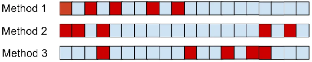
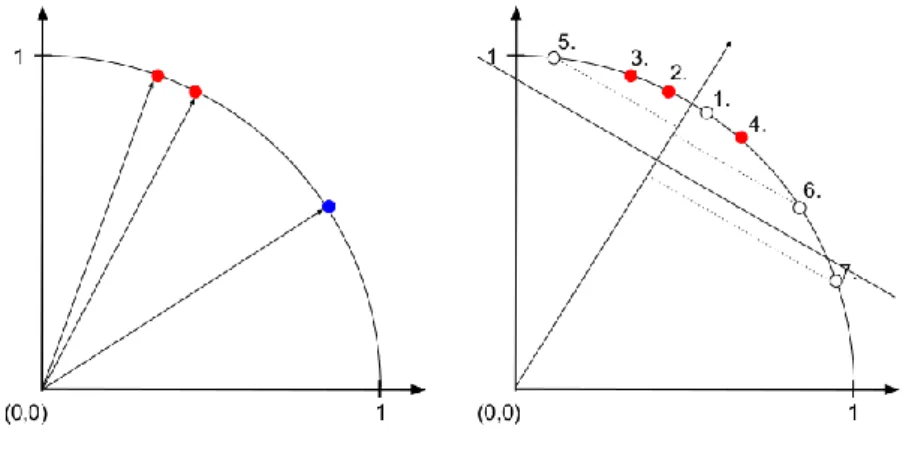
First, we illustrate performance measures in a medicinal chemistry context using a small example. Let us assume we have 20 unknown compounds, 5 out of which are active COX- 1 inhibitor. The fraction of actives (RP) in this dataset is 25%, which is selected for illustrative purposes and unrealistically high in practice. We have three different methods which order these compounds based on the chemical structure and further information we have. After ordering the compounds, we check the COX-1 inhibitory activity of the compounds in vitro, and we get the result on Figure 3.
In this example red colour always indicates active compound and blue indicates inactive compound. In Figure 3 boxes represent compounds in the order the given method ranked them. The question is which method is the best.
The answer, as always, depends on what we mean by 'the best'. To concentrate on performance measures, let us regard these predictors as black boxes, which means there is no use of the predictor on its own; we want to evaluate only the predictive performance of the models. For instance, we cannot learn new chemistry by inspecting them, or we cannot use the models for lead optimization more effectively than just predicting activities of analogues.
If we have limited capacity to test compounds, and we want good candidates for our pipeline, how much can we gain? We will apply a threshold τ to define the position in the
Figure 3 - Output ordering of three hypothetical prioritization methods on 20 compounds: 5 active (red boxes) and 15 inactive compounds (blue boxes). Predicted
activity is highest on the left side and lowest on the right side.
list above which the compounds are predicted to be active. To measure predictive performance we need to define some statistical measures:
True Positive (TP): Number of compounds our classifier predicted as active out of the real active ones.
False Positive (FP): Number of compounds our classifier predicted as active but which actually are inactive.
True Negative (TN): Number of compounds our classifier predicted as inactive out of the real inactive ones.
False Negative (FN): Number of compounds our classifier predicted as inactive, but which actually are active.
All of these four measures are threshold dependent, therefore we could write them as functions as well in the form: TP(τ), FP(τ), TN(τ) and FN(τ) respectively. We will need two parameters of the library, which are independent of the model and the applied threshold:
NP (All Positives): The number of active compounds in our library. NP which applies to our whole library is usually not known, but it can be known in case of a validation set.
NN (All negatives): The number of inactive compounds in our library. The sum of NP and NN is the size of the library NA, and the ratio of actives can be written as RP = NP/NA. As we will see, these numbers will be sufficient to derive all measures we need in a contingency table (Table 2).
Table 2 - Contingency table. Table containing all sufficient statistics we need to assess performance given a threshold τ.
Real active (NP)
Real inactive (NN) Predicted to be
active
True Positive False Positive Predicted to be
inactive
False Negative True Negative
We will use the following derived measures:
Sensitivity (also called Recall): The fraction of the active compounds that the classifier identified successfully. TP / NP
Specificity: The fraction of the inactive compounds that the classifier excluded successfully. TN / NN
Precision (also called Positive Predictive Value): The fraction of real actives, in the set of compounds that the classifier identified as active. TP / (TP + FP)
For a medicinal chemist, precision has a probably more intuitive form called the Enrichment Factor (ER). ER is a normalized form of precision by the fraction of active compounds in the whole dataset. It measures the fold of increase in the number of hits, which the experimenter can get if instead of choosing random compounds from the library, they test compounds predicted by the model. We can write EF proportional to sum of weights for all active compounds [55]:
where the weighting for a compound ranked before the threshold is 1, and after the threshold is 0:
where ri denotes the rank of the active compound i in the output ordering of the model.
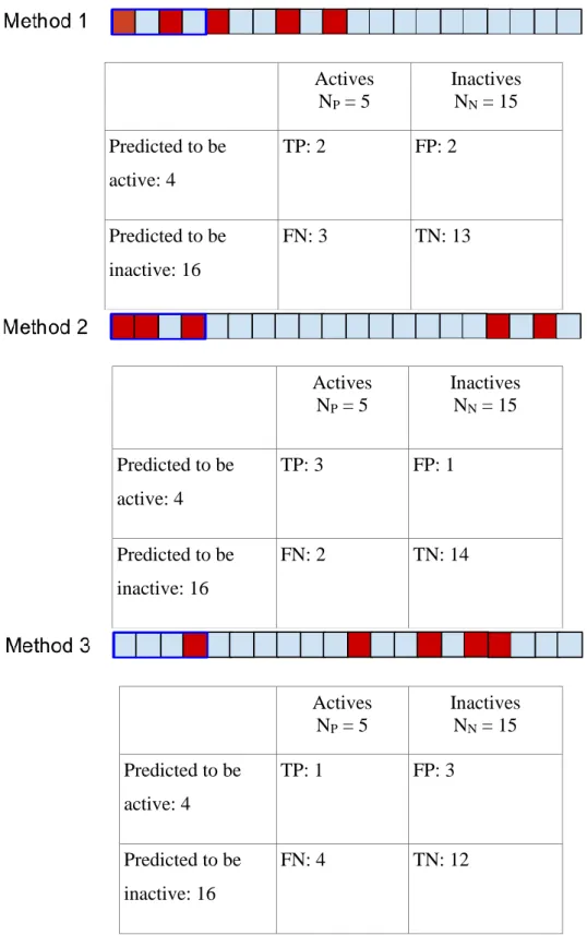
Let us assume that we have capacity to test 4 compounds, so we will use the methods to predict the 4 most likely active compounds (Figure 4).
Actives NP = 5
Inactives NN = 15 Predicted to be
active: 4
TP: 2 FP: 2
Predicted to be inactive: 16
FN: 3 TN: 13
Actives NP = 5
Inactives NN = 15 Predicted to be
active: 4
TP: 3 FP: 1
Predicted to be inactive: 16
FN: 2 TN: 14
Actives NP = 5
Inactives NN = 15 Predicted to be
active: 4
TP: 1 FP: 3
Predicted to be inactive: 16
FN: 4 TN: 12
Figure 4 – Contingency tables and graphical illustration of thresholding for τ = 4
Based on these contingency tables, we can compute the derived measures (Table 3).
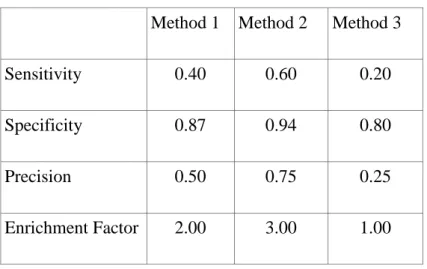
Table 3 - Derived measured computed for τ = 4
Method 1 Method 2 Method 3
Sensitivity 0.40 0.60 0.20
Specificity 0.87 0.94 0.80
Precision 0.50 0.75 0.25
Enrichment Factor 2.00 3.00 1.00
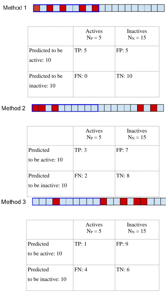
For example, in case of Method 1 40% of the actives (two out of five) has been in the 4 selected compounds, therefore they have been identified successfully, while 87% of the inactive compounds are excluded. The ratio of actives in the 4 selected compounds is 50%, which corresponds to a two fold increase relative to random selection. We can see from Table 3 that the classifier corresponding to Model 2 at the selected threshold outperforms the other two classifiers irrespectively of our optimization goal. For example, this classifier improves our hit rate by 3 folds. While this classifier is objectively better, the same is not true in the level of the methods. Let us choose now a new threshold: we can now test 10 compounds (Figure 5).
Actives NP = 5
Inactives NN = 15 Predicted to be
active: 10
TP: 5 FP: 5
Predicted to be inactive: 10
FN: 0 TN: 10
Actives NP = 5
Inactives NN = 15 Predicted
to be active: 10
TP: 3 FP: 7
Predicted
to be inactive: 10
FN: 2 TN: 8
Actives NP = 5
Inactives NN = 15 Predicted
to be active: 10
TP: 1 FP: 9
Predicted
to be inactive: 10
FN: 4 TN: 6
Figure 5 - Contingency tables and graphical illustration of thresholding for τ =10
The computed derived measures are shown in Table 4.
Table 4 - Derived measures computed for τ = 10
Method 1 Method 2 Method 3
Sensitivity 1.00 0.60 0.20
Specificity 0.67 0.53 0.40
Precision 0.50 0.30 0.10
Enrichment Factor 2.00 1.36 0.40
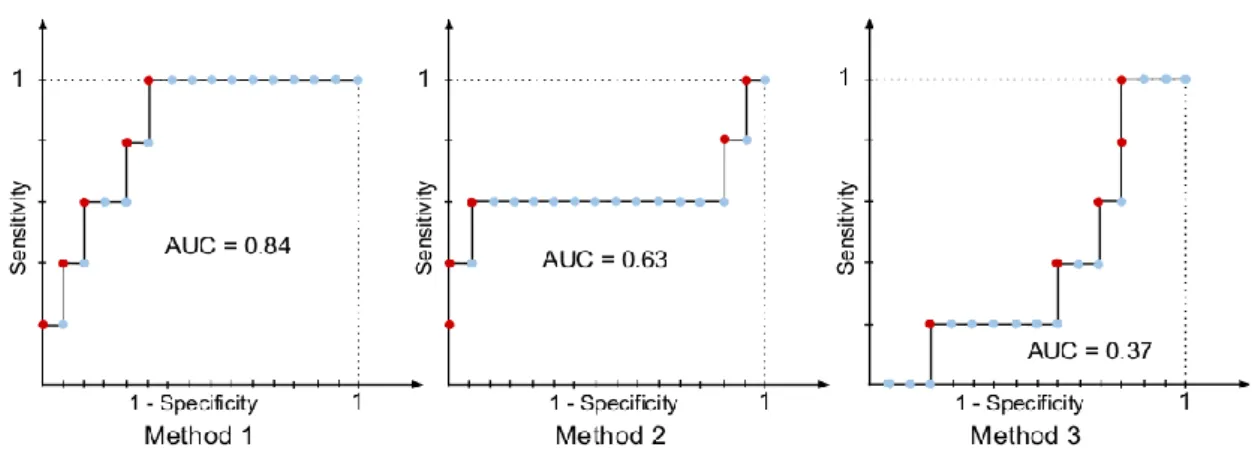
With this threshold the classifier corresponding to Model 1 outperforms the other two classifiers according to all measures. It is clear that the performance of a model we want to use for classification will depend on the threshold, but will not depend on the ordering of the compound above or below that threshold. We can plot this performance for all possible thresholds using a tool called Receiver Operating Characteristic or ROC curve.
As a convention, we plot the sensitivity with respect to 1-specificity for all threshold levels (Figure 6).
In some cases we are interested in the predictive performance of the models in a threshold independent way. One measure to use in this case is the area under the ROC curve (AUC).
The AUC value has a very intuitive interpretation: it gives the probability of ranking an active compound higher than an inactive one if the inactive-active pair in question is drawn uniformly at random. This interpretation relies on the connection between AUC and the Mann-Whitney-Wilcoxon statistics [56].
We can see that according to the AUC measure, Method 1 is better than Method 2, which is better than Method 3. We can also realize that Method 3 would be a bit better if we inverted its ordering. The truth is that the ordering for Method 3 was generated randomly;
and because of the small number of entities, its AUC value can randomly deviate from the totally random model. If we had a huge number of entities, a random model would be a diagonal line with AUC = 0.5. To better understand the apparently controversial statements about Model 1 and Model 2, let us examine the ROC plots of them together (Figure 7, left).
Figure 6 - Receiver Operating Characteristics (ROC) curve of the three different prioritization methods. Every coloured dot corresponds to an active (red) or inactive
(blue) compound in the ordered sequence.
The green ROC curve corresponds to Method 1, and the brown one to Method 2. The green and brown shaded area corresponds to the superiority of Method 1 and 2 respectively. The AUC metric weights the two sub-area equally, Model 1 therefore has higher AUC value.
It can be shown that we can write AUC in the following form:
where ri denotes the rank of the active compound i in the output of the model. From this equation we can see that AUC is a linear transformation of the sum of a weighting, where the weights are:
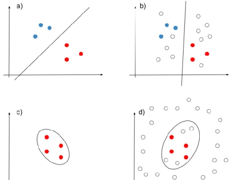
If our chemical library contains several millions of compounds, but we have a limited testing capacity for testing only the top hits – which is the case in practice - , we are usually not interested in the performance after the top hits i.e. in the brown area. We want to weight the early part higher, and only invest time and money in more measurement, if it is really worth it. In this case we are facing the so called early recognition problem. An Figure 7 - Comparison of the Receiver Operating Characteristics (ROC) (left) and the Concentrated ROC curves (right) of Method 1 and Method 2. The green area represents
the superiority of Method 2 in classification tasks using small threshold value, the brown area represents the superiority of Method 1 in case of high threshold values.
intuitive way to do it is to transform the horizontal axis of the ROC curve in such a way, that the area elements in the early part of the curve will be magnified, and in the late part they will be compressed. In a more formal way, we apply a continuous compression function f to 1-specificity, which maps the [0,1] interval to itself, f : [0,1] → [0,1]. An illustration is shown on Figure 7 (right), where we can see that the green area in the low end of the 1-specificity axis is now magnified, while the brown area at the high end is compressed. This type of transformation reflects our preference in the early recognition problem and can be achieved by a concave compression function, which has a derivative higher than 1 for low values, and lower than 1 for high values. This measure is called the concentrated ROC (CROC) [57]. A well-behaving compression function, which we will use in this work is the exponential compression:
This function has a parameter α, which defines how early is the part we want to focus on.
A very similar measure can be derived also form the probability theory point of view, called Boltzmann-Enhanced Discrimination of ROC (BEDROC) [55]. If we enforce that our weighting corresponds to a proper probability density function f(x), than we can interpret our weighted sum in the continuous limit:
as an expected value, which have a similar probabilistic interpretation to AUC given that αNP/NN << 1 holds, which is usually the case in virtual screening, and is the case in our experiments as well.
Similarly to the case of AUC, we need to transform this rank average based metric to get a metric which have values between 0 and 1:
It is important to note that BEDROC is not a measure which tells if our model is better than a random model or not. It tells if our model is better than a reference enrichment, we