Astronomy &
Astrophysics
https://doi.org/10.1051/0004-6361/201834325
© ESO 2019
Secondary eclipse of the hot Jupiter WASP-121b at 2 µ m ?
Géza Kovács1and Tamás Kovács2
1Konkoly Observatory of the Hungarian Academy of Sciences, Budapest, 1121 Konkoly Thege ut. 15-17, Hungary e-mail:kovacs@konkoly.hu
2Institute of Theoretical Physics, Eötvös University, Budapest, 1117 Pázmány Péter sétány 1A, Hungary Received 26 September 2018 / Accepted 3 April 2019
ABSTRACT
Ground-based observations of the secondary eclipse in the 2MASSKband are presented for the hot Jupiter WASP-121b. These are the first occultation observations of an extrasolar planet that were carried out with an instrument attached to a 1 m class telescope (the SMARTS 1.3 m). We find a highly significant eclipse depth of (0.228±0.023)%. Together with other planet atmosphere measurements, including theHubbleSpace Telescope near-infrared emission spectrum, current data support more involved atmosphere models with species producing emission and absorption features, rather than simple smooth blackbody emission. Analysis of the time difference between the primary and secondary eclipses and the durations of these events yields an eccentricity ofe=0.0207±0.0153, which is consistent with the earlier estimates of low or zero eccentricity, but with a smaller error. Comparing the observed occultation depth in theKband with the one derived under the assumption of zero Bond albedo and full heat redistribution, we find that WASP-121b has a deeper observed occultation depth than predicted. Together with the sample of 31 systems withK-band occultation data, this observation lends further support to the idea of inefficient heat transport between the day and night sides for most of the hot Jupiters.
Key words. planets and satellites: atmospheres – methods: data analysis
1. Introduction
When it is combined with other pieces of information (such as planet mass), the low thermal radiation of extrasolar planets is direct evidence of their substellar nature. In addition to this inde- pendent verification, measuring the radiation spectrum yields a wealth of information on atmospheric structure and basic orbital parameters. Because of their low temperatures (relative to the temperatures of their host stars), the best chance of detection clearly lies in the infrared. From the first detection, employing the mid-infrared instrument of the SpitzerSpace Telescope by Deming et al.(2005), many systems have been observed not only by space-based, but also by ground-based instruments attached to 4-m class telescopes. Here we report the multiple detection of the secondary eclipse1 of the hot Jupiter (HJ) WASP-121b in the 2MASS K band by A Novel Dual Imaging CAMera (ANDICAM) attached to the 1.3 m telescope of the SMARTS Consortium2.
The transiting extrasolar planetary system WASP-121 was discovered by Delrez et al. (2016) using the wide-field tele- scopes of the SuperWASP project (Pollacco et al. 2006, see also Anderson et al. 2018for the latest update). The analysis of these and the subsequent spectroscopic followup observations revealed that WASP-121b is a very hot Jupiter, with a maximum pho- tospheric temperature above 3000 K. This is expected because the planet very closely orbits an F star (Porb =1.27 days). The
?Photometric time series are only available at the CDS via anonymous ftp to cdsarc.u-strasbg.fr (130.79.128.5) or via http://cdsarc.u-strasbg.fr/viz-bin/qcat?J/A+A/625/A80
1 Throughout this paper, we also use the word “occultation” for the event of secondary eclipse.
2 For additional details on the instrument, access images, seehttp://
www.astro.yale.edu/smarts/1.3m.html;http://archive.
noao.edu/search/query/
close orbit and the extended planet radius3 of Rp = 1.87 RJ
with a standard mass ofMp =1.18MJimply rather strong tidal dissipation, leading to Roche-lobe filling and then to a speedy disruption within some hundred million years, assuming a stel- lar tidal dissipation factorQstar<108(seeDelrez et al. 2016; and for the signature of a strongly evaporating atmosphere, the near- UV observations ofSalz et al. 2019). In addition, the planet has probably experienced a strong dynamical interaction with some nearby third body, as can be inferred from the large projected spin-orbit angle of 258◦±5◦ (seeDelrez et al. 2016). Interest- ingly, secondary eclipses were observed multiple times by the same authors in the Sloan-z0band by the 60 cm TRAPPIST tele- scope; to our knowledge, this is the first occultation detection from the ground by a telescope of this size. The significant detec- tion of the occultation depth of a mere (0.060±0.013)% resulted in the first direct estimation of the planet temperature. Important followup observations (both during the primary and secondary eclipses) have been made by Evans et al. (2016, 2017, 2018) using theHubbleSpace Telescope’s (HST) Wide Field Camera 3 in the near-infrared, theSpitzer/IRAC detector at 3.6µm, and HST/STIS in the UV. These data indicate a weak H2O emission during occultation and absorption during transit, implying tem- perature inversion due to some high-altitude absorber. In spite of the successful fit of the HST emission spectrum, and quite currently the transmission spectrum observed by the same instru- ment, the authors caution that the solution is not unique (e.g., type of absorber and precision of the fit at different wavelengths).
These issues are not unique to WASP-121b, they are also present in other very hot Jupiters (e.g., WASP-33b, Kepler-13Ab; see Parmentier et al. 2018). In spite of the considerable progress
3 The radius quoted here is the one that appears in the abstract of the discovery paper. We use the radius based on the HST measurements of Evans et al.(2017); see Sect.4.
Table 1. Secondary eclipse observations of WASP-121b in the near- infrared.
Date (UT) Tocc(HJD) Ttot(h) Ntot
02/26/2016 2457444.64855 4.86 177 01/11/2017 2457764.65485 6.13 203 01/25/2017 2457778.67903 6.64 205
Notes.Toccstands for the time of the center of occultation as estimated from the ephemeris given byDelrez et al.(2016) for the primary eclipse in their Table 4.TtotandNtotare the total observing time and gathered data points.
made in the past ten years, there is a substantial lack of under- standing the relations between the physical parameters of the systems and the thermal properties of their planets (see the uni- form analysis byAdams & Laughlin 2018 of ten systems with full infrared phase curves).
The purpose of this work is to add a flux value to the emis- sion spectrum of WASP-121b at a single waveband and thereby increase the number of constraints on future atmosphere mod- eling of the planet. Furthermore, timing estimates are presented to give more stringent limits on the orbital eccentricity, which is a valuable parameter for analyzing the dynamical history of the system.
2. Observations and analysis method
Photometric observations in the 2MASSKand CousinsIbands (effective wavelengths of 2.2 and 0.8µm, respectively) have been made by using the ANDICAM instrument in a beam-splitting mode, allowing simultaneous data acquisition in the two bands4. On each night, the target was monitored continuously, by allow- ing ample amount of pre- and after-event time (permitted by the actual sky position) to reliably fix the out-of-eclipse (OOE) baseline for the event, which lasted for almost 3 h. An expo- sure time of 15–20 s was used, resulting in an overall cadence of 70–500 s because of the overheads, related to read-outs, vary- ing movements due to dithering, and other data acquisition steps.
The observing log with some associated parameters is given in Table1.
For theK-band observations, dithering was used to decrease the higher sensitivity against detector non-uniformity in the near- infrared. We found this method useful because we did not have a priori information on pixel sensitivity. This method also includes some risk, however, because by testing different parts of the CCD, we may bump into bad positions, leading to light curves of larger scatter that is associated with the particular dither posi- tion. Our strategy has proven to be useful in general and led to a higher quality result in the end.
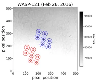
By stacking several images, we show the dither pattern in Fig. 1 for one of the nights. The number of dither positions changed from night to night, and their durations varied. The image (already corrected for flat field) spectacularly exhibits sequences of rings, which are reminiscent of the trace of ear- lier dewdrops. In spite of their high visibility, their effect has been proven to be less damaging for the data quality than the
4 Unfortunately, the signal, hampered by weather and instrumental limitations, in the CousinsIband was too weak to yield any useful plan- etary atmospheric constraint, so we decided to discard it. The expected occultation depth in this band is ∼0.5 ppt, yielding a less than 3σ detection with the data at hand.
0 100 200 300 400 500
pixel position
0 100 200 300 400 500
pixel position
WASP-121 (Feb 26, 2016)
75000 80000 85000 90000 95000
counts
Fig. 1. Dithering pattern used during the near-infrared observations.
The image shows the 2.40×2.40FOV of the ANDICAM near-infrared camera, attached to the 1.3 m telescope of the SMARTS Consortium.
The target (WASP-121=2MASS 07102406-3905506) is in the middle, the comparison star 2MASS 07102364-3905561 is in the lower left cor- ner. North is up and west is to the left. Circles around the target and the comparison star show the aperture sizes used to estimate the stellar and background fluxes.
0.97 0.98 0.99 1.00 1.01 1.02 1.03 1.04
0.40 0.45 0.50 0.55 0.60 0.65
FLUX
PHASE
#13
#9
#6
#6
Fig. 2.Simple photometric flux ratios ordered by the orbital period (pale dots). Some dithers are annotated to show the nightly trends (or the lack of them, i.e., number 9). Dither 6 (gray dots) is plotted also after employing zero-point shift and detrending by the position vector (black dots, see Sect.2for details).
varying pixel sensitivity (which is considerably more difficult to spot because the pixels lack the type of spatial correlation that the rings have).
To produce the photometric time series that was to be used to derive the basic occultation parameters, we proceeded as fol- lows. First we computed simple relative fluxes at various but fixed circular apertures from 10 to 20 pixel radii with an incre- ment of 2 pixels. After much experimenting and inspecting the final product of the full detrending procedure to be described below, we find that an aperture with a pixel radius of 16 yields the light curve with the smallest scatter. All results presented in this paper refer to this aperture size.
By using the relative fluxes (target over comparison star flux, hereafter raw flux) and folding the data with the orbital period, we can determine whether we can see some sign of an occulta- tion event. The result is shown in Fig.2. The pale dots show that the raw fluxes are very noisy, and the event with the expected depth of 0.1–0.2% is hopelessly buried in the noise. We can determine the reason of this somewhat unexpected high level
of noise by examining the individual light curves associated with the various dither positions5. The highlighted light curves show a strong dependence on the dither position, leading to both zero-point shifts and nightly trends. Therefore (not entirely unex- pectedly), we must employ some detrending method that is likely the cause of the trends and zero-point shifts. The detrending step is vital and therefore quite common in the extraction of planetary signals in general, and in particular, in deriving wavelength- dependent transit depths for the exquisite accuracy needed to estimate emission or transmission spectra (e.g.,Stevenson et al.
2012;Kreidberg et al. 2015).
It is well known that ground-based instruments detect stellar light deformed by the multiplicative noise and systematics orig- inating from the Earth’s atmosphere and from the environment or instrument. In addition, we also have an additive noise source from the sky background,
F=F0×Tatm×Tenv+Fbg, (1) whereFis the detected andF0is the true stellar flux. The trans- mission functions of the Earth’s atmosphere and the instrument are denoted byTatm andTenv, respectively, and the background flux is given by Fbg. In traditional photometric reductions the atmospheric and instrumental effects are filtered out with the aid of comparison stars near the target, using the assumption of the close similarity in the transmission functions for the target and its neighboring companions. However, when higher accu- racy is required, this method usually fails because of the lack of complete equivalence between the transmission functions of the target and the comparison stars (for faint targets, the additive background noise is an additional problem).
Because we lack an obvious exact solution of the problem (similarly to the method followed in other studies, e.g., Bakos et al. 2010;Delrez et al. 2016), we opted for an approximate solu- tion. Here we took the logarithm of the target to comparison star flux ratiosF/Fc, and fit the data with the linear combination of the presumed signal and certain external photometric parame- ters (e.g., position, and width of the point spread function, PSF).
In addition, we treated each light curve of the different dither positions individually, with particular zero-points and trends (but with the same underlying signal). That is, we used a least-squares minimization for the following expression:
D=
M
X
j=1 Nj
X
i=1
wj
log Fj(i) Fjc(i)
!
−Ej(i) 2
, (2)
Ej(i)=a0,j+ax,jXj(i)+ay,jYj(i)+Alog(Ftrap(i)). (3) Here all data were sorted by the orbital phase. We assumed that there are M dither positions altogether withNjdata points at the jth dither. Because our extensive tests showed that nei- ther arbitrary polynomial nor additional external parameters are needed to reach a detection with a high signal-to-noise ratio (S/N), we only used the pixel position components (X,Y) of the target to correct for instrumental effects. The stellar flux during the occultation was approximated by a trapezoidal functionFtrap
with fixed ingress and egress time, duration, and eclipse center of 0.015, 0.120 and 2457764.65485 days, respectively, corre- sponding to those given by Delrez et al. (2016). The weights {w} were constant for the same dither index and proportional to the reciprocal of the variance of the residuals around the best-fitting trapezoidal. Because the solution was not known, the
5 All dither positions were counted, and their indices increase toward more recent nights of observation.
Table 2.Occultation depths for WASP-121 in the 2MASSKband.
Ndithcut Nσcut Npar N S/N σfit δocc
0 ∞ 70+ 0 585 8.1 0.00272 0.00212
0 5 70+ 8 585 8.4 0.00264 0.00215
0 4 70+11 585 8.8 0.00264 0.00224
0 3 70+25 585 9.2 0.00256 0.00227
10 ∞ 61+ 0 561 8.2 0.00275 0.00217
10 5 61+ 8 561 8.5 0.00266 0.00220
10 4 61+11 561 8.9 0.00266 0.00228
10 3 61+25 561 9.3 0.00257 0.00231
15 ∞ 52+ 0 520 8.2 0.00281 0.00231
15 5 52+ 8 520 8.6 0.00270 0.00233
15 4 52+11 520 8.9 0.00270 0.00243
15 3 52+25 520 9.3 0.00260 0.00244
Notes. Ndithcut is the minimum number of data points per dither posi- tion before sigma clipping.Nσcutis the number of standard deviations used in clipping the data points.Nparis the number of parameters fitted, plus the number of omitted data points (Npin Eq. (4) includes both of these). Items in the last two columns (unbiased estimates of the standard deviation of the residuals and occultation depth) refer to the OOE=1 normalization as described in Sect.2.
weights were iterated during the process of solution. Finally, the data were converted back into relative intensities, with an OOE normalization of 1.0 for the fitted trapezoidal. The error of the occultation depth was computed as
σ(δocc)= 1−Np
N
!−1/2 s14 N142 + sooe
Nooe2
!1/2
, (4)
wheres14andsooeare sums of the squared residuals in the in-the- eclipse and OOE phases, respectively, with associated number of data pointsN14andNooe. The factor in front (withNpparameters fitted toNdata points) represents the debiasing of the error due to the decrease of the degrees of freedom, because of parameter fitting. The S/N of the detection is the ratio of the average eclipse depth to this error,
S/N= 1 σ(δocc)
1 N14
N14
X
i=1
Ftrap(i). (5)
3. Occultation parameters
First we fixed all secondary eclipse parameters (except for the occultation depth) by assuming a circular orbit and the validity of the parameters derived for the transit byDelrez et al.(2016).
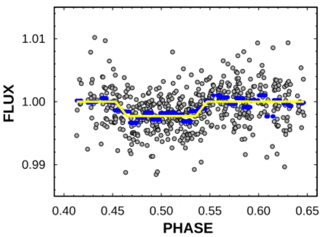
Following the procedure described in Sect.2, we computed the best-fitting occultation depth under various conditions, concern- ing the number of clipped points and the omitted dither light curves. The result is shown in Table2. Except perhaps for the extreme choices of data trimming parameters (Ndithcut and Nσcut), the occultation depth is relatively stable. To avoid too sparsely populated dither light curves and to avoid overtrimming the data, we opted for the case of Ndithcut =10 and Nσcut =4. The folded light curve obtained in this way is shown in Fig.3. The resulting secondary eclipse depth is 0.00228±0.00023.
To determine the level of the systematics filtering, we com- puted the autocorrelation function (ACF) of the residuals after subtracting the best-fitting trapezoidal as shown in Fig. 3. In units of the orbital period, the ACF was computed with steps
0.99 1.00 1.01
0.40 0.45 0.50 0.55 0.60 0.65
FLUX
PHASE
Fig. 3. Systematics-filtered folded flux ratios normalized to 1.0 in the OOE part. Average fluxes (in 30 phase bins) are shown by blue dashes, and the best-fitting trapezoidal secondary eclipse approximation is plotted as the yellow continuous line.
-0.2 0.0 0.2 0.4 0.6 0.8 1.0
0.00 0.02 0.04 0.06 0.08 0.10 0.12
Shift [phase]
Normalized correlation
0.0 0.4 0.8
0.000 0.005 0.010
Fig. 4.Blue dots: autocorrelation function (ACF) of the residuals of the trapezoidal fit to the final dataset shown in Fig.3. Red dots: ACF of generated uncorrelated noise. Error bars are for the standard deviations of the ACF values of the random datasets. The time lag is given in units of the orbital period. The inset shows the immediate neighborhood of ACF at zero time-shift.
of 0.00123 up to 0.115, that is, close to the length of the full eclipse event. As a sanity check, we also computed the ACF for many Gaussian white-noise realizations. The result is shown in Fig.4. The residuals are almost uncorrelated. The basic cor- relation length is smaller than ∼0.005 in units of the orbital period. This value is lower than one-half of the ingress dura- tion. It seems that the decorrelation method we applied yields nearly white-noise residuals, which supports the validity of the pure statistical error estimation given by Eq. (4). We also note that similar short-timescale correlations are observable in other studies that investigated systematics, in particular, in the analysis of the HST data byEvans et al.(2017).
Although the noise is rather high, the relatively large number of data points led to a detection with high S/N. Therefore, it is tempting to examine whether our assumption on the applicability of the transit parameters holds, and if there is a way to further constrain the eccentricity by the best-fitting occultation center and event duration. To this aim, we mapped the quality of the fit as a function of∆Tc(tested occultation center time minus the one calculated from the transit with the assumption of circular orbit) andt14 (occultation duration).
-0.02 -0.01 0 0.01 0.02
0.1 0.11 0.12 0.13 0.14
t14 [d]
∆Tc [d]
6.9e-06 7e-06 7.1e-06 7.2e-06 7.3e-06 7.4e-06 7.5e-06 7.6e-06
SMARTS 2MASS K
Fig. 5.Intensity plot for the unbiased estimate of the variance of the residuals between the data and the occultation model scanned in the parameter space of the displacement of the occultation center∆Tcand the duration of the eventt14. We employ iterative 4σclipping to find the best solution for each parameter combination.
-0.02 -0.01 0 0.01 0.02
0.1 0.11 0.12 0.13 0.14
t14 [d]
∆Tc [d]
1.017e-05 1.018e-05 1.019e-05 1.02e-05 1.021e-05 1.022e-05 1.023e-05 1.024e-05
TRAPPIST Sloan z’
Fig. 6.Same as in Fig.5, but for the TRAPPIST data. The better contrast of the best solution is attributed to the significantly larger number of data points for the TRAPPIST data.
To further examine the issue of eccentricity, the secondary eclipse data ofDelrez et al.(2016) were investigated in addition to our data. Because the observations were made in the Sloanz0 band, the signal is considerably shallower than in the 2MASS K (Ks) band. Nevertheless, the number of data points (6260 flux measurements on seven nights) compensates for this, and yields a confident detection of S/N = 7.5, with δocc = 0.000697± 0.000081 and a residual standard deviation of 0.003190. This depth is larger by 0.000096 than the one derived byDelrez et al.
(2016), but the difference is within 1σ, and could be accounted for by the lower number of detrending parameters used in our code. We found it satisfactory to use only the pixel coordinates, and avoid correcting with a polynomial and other parameters because these do not yield an appreciable improvement in the quality of the fit and may in addition lead to a depression of the occultation depth.
The (∆Tc,t14) maps are shown in Figs.5and6for the Ks
and Sloan z0 data, respectively. As expected, the topology of both maps confirms the rather small (if any) deviations from the parameters predicted by the transit with the assumption of circu- lar orbit. Furthermore, the Sloanz0data are more restrictive than the Ks data, even though the S/N value is higher for the latter.
This is because the parameter maps also yield information on the sensitivity of the solution on the neighboring parameter val- ues and not only on a specific combination of the parameters, which might be better or worse, depending on the functional
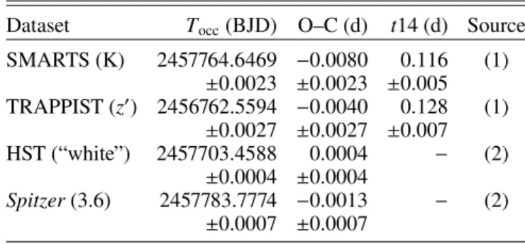
Table 3.Observed secondary eclipse times for WASP-121b.
Dataset Tocc(BJD) O–C (d) t14 (d) Source SMARTS (K) 2457764.6469 −0.0080 0.116 (1)
±0.0023 ±0.0023 ±0.005 TRAPPIST (z0) 2456762.5594 −0.0040 0.128 (1)
±0.0027 ±0.0027 ±0.007 HST (“white”) 2457703.4588 0.0004 − (2)
±0.0004 ±0.0004
Spitzer(3.6) 2457783.7774 −0.0013 − (2)
±0.0007 ±0.0007
Notes.The source of the TRAPPIST data isDelrez et al.(2016). The O–C values are computed with respect to the ephemerides predicted from the transit as given by Delrez et al.(2016), assuming a circular orbit. See text for the equality of the errors onTocc and O–C.Evans et al.(2017) did not supply occultation duration values.
References.(1) This paper; (2)Evans et al.(2017).
form of the variance on these parameters and noise level. The better quality of the Sloan z0 data is also visible in the nearly three times smaller error of the derived occultation depth.
The currently available secondary eclipse parameters are summarized in Table3. The errors of the items associated with this paper have been computed in the following way. After the best-fitting trapezoidal was found, we added Gaussian white noise with the observed standard deviations of the residuals corresponding to this solution, and then the best-fitting trape- zoidal to these simulated data was searched for. By repeating the process 500 times, we computed statistically stable estimates of the formal errors. The ingress and egress time was always fixed to the observed values given by the transit data ofDelrez et al.(2016), and we repeated this with the remaining parame- ters, depending on which parameter was tested for errors (e.g., in the case of the occultation center, we fixed the duration and the ingress and egress times). Although this approach is primarily dictated by keeping the execution time within a reasonable limit, our error estimates for the moment of the occultation time is in perfect agreement with the one predicted by the analytic formula ofDeeg & Tingley(2017). The errors of O–C were taken equal to those ofToccbecause the errors of the computed occultation times (C) have been proven to be negligible.
The available observations suggest a small (or zero) eccen- tricity. Because the more precise estimation also requires knowl- edge of the eclipse duration, the lack of this parameter for the most accurate HST and Spitzer observations prevents us from including these data in the analysis. Therefore we used only the occultation parameters derived from the SMARTS and TRAPPIST observations.
Following Winn (2010), by omitting the negligible incli- nation effect, we use the following formula to estimate the eccentricity:
e=
" π 2
∆Tc
P
!2
+ r14−1 r14+1
!2#12
, (6)
where P is the orbital period,∆Tc is the observed time of the occultation center minus the predicted time from the transit, assuming zero eccentricity;r14=t14(occ)/t14(tra), which is the ratio of the secondary and primary eclipse durations.
Assuming that the errors are independent of the eclipse times and durations both for the primary and the secondary eclipses
and that these errors are also uncorrelated with the error of the period, we can use this equation to estimate the eccentricity and its pure statistical error.
For the transit and for the period, we took the values given in Table 4 of Delrez et al. (2016). For the secondary eclipse, we used the values shown in Table3of this paper. Errors were assumed to be Gaussian. Then, Eq. (6) yields e = 0.0207± 0.0153 when we use the SMARTS and e =0.0314±0.0222 when we use the TRAPPIST data. These eccentricity values were also tested using the transit center values of Evans et al.
(2018) for the HST/STIS G430Lv2 band (we obtained very simi- lar results for the other bands as well). We note that this test is not entirely consistent because we used the transit duration value of Delrez et al.(2016):Evans et al.(2018) did not give this param- eter for their data. We obtain for the SMARTS and TRAPPIST datae=0.0198±0.0157 ande=0.0312±0.0224, respectively, that is, very close to the values estimated on the basis of the transits ofDelrez et al.(2016).
Concluding, we note that Delrez et al.(2016) quoted a 3σ upper limit of e=0.07 from the global analysis of the photo- metric and radial velocity data. Our independent analysis agrees quite well with theirs.
4. Comparison with planet atmosphere models At the time of writing, the following secondary eclipse observa- tions are available for WASP-121b: the Sloanz0data at 0.9µm byDelrez et al.(2016), and the HST data in 1.1–1.6µm and the Spitzerdata at 3.6µm, both by Evans et al.(2017). The main panel in Fig. 7 shows these two single-band data points, the band-averaged value of the HST spectral data, and our occul- tation depth in theK band at 2.2µm (see also Table4 for the actual numerical values we used). The data are overplotted on the recent planetary atmosphere models ofEvans et al.(2017) and Parmentier et al.(2018). We note that although the “No dissocia- tion” model very clearly shows that element dissociation needs to be considered in modeling HJ atmospheres, it is unphysical, and it is included merely to show the extreme case of neglecting this important physical process. This model was constructed using chemical equilibrium chemistry in the atmospheric structure module of the global circulation model, but the H2O abundance was considered fixed in computing the spectrum. However, the model labeled “Solar composition” is consistent in this respect and shows that the currently available data overall agree with it6, without any special assumption or adjustment. Unfortunately, the situation is somewhat more involved because several other pos- sibilities yield spectra that are rather similar to that of the “Solar composition” model. For example, the heavy metal content of the “Solar composition” model might be increased by a factor of three, without any essential effect on the emission spectrum; see Parmentier et al.(2018) for further details.
The blackbody lines (gray and black) in Fig.7show the effect of heat transport from the day to the night side. When we assume zero Bond albedo in both cases, the black line displays the case of heat transport with maximum efficiency (AB=0,ε=1.0; see Cowan & Agol 2011;Lopez-Morales & Seager 2007). It is clear that all available data exclude this possibility and support cir- culation models that are rather inefficient, resulting in a higher day-side temperature. For WASP-121b, this temperature seems to be close to 2700 K, corresponding toε=0.57, assumingAB=0.
In a comparison with the models ofEvans et al.(2017), who also
6 By admitting the existence of systematic differences for the HST near-infrared measurements ofEvans et al.(2017); see inset of Fig.7.
0 1 2 3 4 5 6
1 2 3 4
Wavelength [µm]
Fp/Fs [ppt]
No dissociation [Par18]
Solar composition [Par18]
Black body 2700K Black body 2360K Retrieved [Eva17]
1.0 1.5 2.0
1.0 1.5 2.0
HST/WFC3
Fig. 7.Comparison of the single-band secondary eclipse depths (includ- ing the band-averaged HST/WFC3 data, turquoise dot) with the plane- tary atmosphere models ofParmentier et al.(2018) [Par18] andEvans et al. (2017) [Eva17]. Vertical error bars show 3σ statistical uncer- tainties, and horizontal bars indicate the widths of the individual wavebands. We caution that the “No dissociation” model is unphysi- cal, and is shown merely to highlight the effect of omitting dissociation in computing the spectrum (see text for further details). The blackbody lines correspond to different efficiency of the day and night heat trans- port (black: fully efficient; gray: no heat transport). For completeness, the inset shows the HST observations ofEvans et al.(2017) with their spectrum retrieval model and the solar composition model of [Par18].
For better visibility, we use 1σerror bars here.
Table 4.Secondary eclipse depths of WASP-121b.
Instr./Filter λc(µm) δ(ppt) σ(δ) (ppt) Source
TRAPPIST (z0) 0.9 0.697 0.081 (3)
HST/WFC3 1.4 1.132 0.036 (2)
2MASS K 2.2 2.280 0.230 (1)
Spitzer/IRAC 3.6 3.670 0.130 (2) Notes.Including the broadband HST/WFC3 data, only single-band data are shown at central wavelengthsλc.
References.(1) This paper; (2)Evans et al.(2017), their Extended Data Table 1; (3)Delrez et al.(2016).
used this planet temperature, we find that their “retrieved” model slightly underestimates our occultation depth by 1.7σ, but the mismatch for the blackbody line of 2700 K is only 0.4σ.
By scanning the planet temperature, we find that the best- fitting blackbody model to the four single-band data points (weighted equally, and also using the broadband value at 1.4µm derived from the HST/WFC3 spectrum byEvans et al. 2017) is reached whenTp =2652 K. The RMS and theχ2 value of the residuals is 0.170 ppt and 17.6, respectively. All points are within or close to 1σ, except for the point at 0.9µm, which deviates by 3.8σ. For the solar composition model ofParmentier et al.
(2018), we obtain 0.234 ppt and 41.2 for the RMS andχ2, respec- tively. These high values result from theSpitzerand HST/WFC3 data, with deviations of 3.2σand 5.6σ, respectively (the other two points deviate by less than 0.5σ). Repeating the same com- parison for the retrieved model ofEvans et al.(2017), we obtain 0.222 ppt and 26.4 for the RMS andχ2. Now all points deviate near 1σ(the 2.2µm point by 1.7σ), except for the HST/WFC3 point, which deviates by 4.7σ. From these tests it seems that there is no strongly preferred model by the single-band data. The preferred status of the blackbody model is due to the adjusted
planet temperature, which turned out to be lower by 50 K than the one used by the detailed atmospheric models. The nearly common outlier status of the HST/WFC3 band-averaged point7 indicates both the value of precise observational data in select- ing the best-fitting atmosphere model and the caution we must take using broadband data because at higher wavelength resolu- tion, the data fit the retrieval model ofEvans et al.(2017) quite well.
It is important to note that the status of the outliers might change with a different way of handling systematics. As men- tioned, overcorrecting the systematics may lead to a lower occultation depth (e.g., we obtained a greater depth from the 0.9µm data by∼0.1 ppt than the depth derived byDelrez et al.
2016, quite likely because our derivation lacked polynomial correction).
Concerning the slightly preferred retrieval model ofEvans et al.(2017), the fact that our measurement deviates by 1.7σfrom their model spectrum indicates that although additional fine- tuning is needed, the basic characteristics of the observations are matched well. On the other hand, the required VO abundance is some thousand times the solar value, which warrants some cau- tion (seeEvans et al. 2017andParmentier et al. 2018for further discussion of this issue with the emission spectrum).
Additional complications come from the more extensive data that are available from HST and ground-based transmission spectrum measurements. The recent analysis of these data by Evans et al.(2018) lends further support to a high (10–30-times solar) VO abundance and lack of TiO. Furthermore, these data also pose some challenges in explaining the steep rise of the absorption in the near-ultraviolet regime. (Which trend if further amplified by the recent near-ultraviolet data by theSwiftsatel- lite; seeSalz et al. 2019.) Evans et al.(2018) invoked sulfanyl (SH) as a possible absorber because the standard explanation by Rayleigh scattering fails in the case of WASP-121b, due to the high atmospheric temperature that is implied by Rayleigh scattering only.
Unfortunately, the currently available data on WASP-121b populate the more easily measurable part of the emission spec- trum still too sparsely. In the waveband between 2 and 4µm (where the CO and H2O emissions are the most pronounced) additional data would be of great help. High S/N measure- ments carried out by instruments such as CRIRES at the Very Large Telescope (VLT) would be clearly capable to map this crucial region. In addition to determining the abundances of the molecules above, this might also constrain the abundances derived from the shorter wavelength part of the spectrum, where gathering data with high S/N is more difficult.
5. Inefficiency of the day- to night-side heat transport
In agreement with other studies (e.g.,Adams & Laughlin 2018, and references therein), our data support the lack of efficient day- to night-side heat transport (see Fig.7). This conclusion is further strengthened when we compare the predicted and observed occultation depths using all currently available data.
Based on the list ofAlonso(2018), we collected the secondary eclipse depths measured in the 2MASS K band for 32 hot Jupiters (seeCroll et al. 2015;Cruz et al. 2015;Zhou et al. 2015,
7 It is important to note that we used the errors given byEvans et al.
(2017) estimated by considering only the statistical errors. However, the true range of the fluxes is nearly twenty times larger, implying the inadequacy of the statistical errors in this case.
0.0 1.0 2.0 3.0
0.0 1.0 2.0
δcal [ppt]
δobs [ppt]
Fig. 8. Observed vs. calculated secondary eclipse depths for the 32 extrasolar planets known today with emission measurements at
∼2.2µm. Nearly all observations lie above the equality line, correspond- ing to the calculated and expected blackbody value, assuming effective heat transport from the day to the night side. WASP-121b is shown as a red square. Error bars show 1σstatistical errors.
Martioli et al. 2018; and this paper). The observed depths as a function of the expected value (assuming zero Bond albedo and fully efficient heat transport) are shown in Fig. 8. The figure clearly shows a nearly uniform offset, with no apparent depen- dence on the expected depth. The effect is exacerbated if we consider more realistic albedos, as suggested by recent analyses of full-orbit phase curves; seeAdams & Laughlin(2018).
We arrive at a similar conclusion when we examine the dif- ference between the observed and calculated occultation depths as a function of the temperature at the substellar point, for instance. Although we admit that a more complete characteriza- tion of the heat distribution by directly measuring the night- and day-side fluxes is required (i.e., Komacek & Showman 2016), no correlation seems to exist between the heat redistribution efficiency and planet temperature based on the 2.2µm measure- ments alone (seeCowan & Agol 2011;Komacek & Showman 2016 advocating the existence of such a correlation). In sup- port of our result, it is interesting to note that a similar study by Baskin et al. (2013), based on Spitzer3.6 and 4.5µm data, has led to the same conclusion.
6. Conclusions
We presented the first secondary eclipse measurements of an extrasolar planet in the near-infrared using a 1 m class telescope.
With the ANDICAM imager attached to the 1.3 m telescope of the SMARTS Consortium, we detected an occultation depth of (0.228±0.023)% in the 2MASSKband from observations made in three nights of the very hot Jupiter WASP-121b. We com- pared this value with theoretical planetary spectra ofParmentier et al.(2018) andEvans et al.(2017) and found that it perfectly fits the former model, using solar composition, atmospheric
circulation, and molecular dissociation. However, when all avail- able secondary eclipse data are considered (Sloanz0, HST and Spitzerdata; see Delrez et al. 2016 andEvans et al. 2017), it seems that the VO-enhanced model of Evans et al. (2017) is preferred over the solar composition model, but with a less favor- able match to our data. Although the 2700 K blackbody line also yields an acceptable overall fit to the available data, the more detailed HST spectrum is not reproduced well. Additional data in the (2–4)µm regime would be very useful to verify model pre- dictions on CO and H2O emissions and build a more coherent planet atmosphere model.
Although our observations were made in a single waveband, they yield a reasonably solid piece of information on both the orbital and atmospheric characterization of the WASP-121 sys- tem. Together with future emission data in the (2–4)µm band, they will allow us to prove or refute the existence of the CO, H2O emission feature on the day side that is predicted by the models in this waveband.
Acknowledgements.We thank Laetitia Delrez for sending us the secondary eclipse observations presented in the discovery paper on WASP-121. We are grateful to Vivien Parmentier for making the relevant planet atmosphere models accessi- ble to us and helping in comprehending the models. The professional help given by the SMARTS staff at the Yale University during the data acquisition period is much appreciated. We also thank the referee for the critical notes on our early interpretation of the planet atmosphere models. The observations have been supported by the Hungarian Scientific Research Fund (OTKA, grant K-81373).
T.K. acknowledges the support of Bolyai Research Fellowship. Additional grants (PD 121223 and K 129249) from the National Research, Development and Innovation Office are also acknowledged.
References
Adams, A. D., & Laughlin, G. 2018,AJ, 156, 28
Alonso, R. 2018,Handbook of Exoplanets(London: Springer)
Anderson, D. R., Temple, L. Y., Nielsen, L. D., et al. 2018, MNRAS, submitted, [arXiv:1809.04897]
Bakos, G. Á., Torres, G., Pál, A., et al. 2010,ApJ, 710, 1724 Baskin, N. J., Knutson, H. A., Burrows, A., et al. 2013,ApJ, 773, 124 Cowan, N. B., & Agol, E. 2011,ApJ, 729, 54
Croll, B., Albert, L., Jayawardhana, R., et al. 2015,ApJ, 802, 28 Cruz, P., Barrado, D., Lillo-Box, J., et al. 2015,A&A, 574, A103 Deeg, H. J., & Tingley, B. 2017,A&A, 599, A93
Delrez, L., Santerne, A., Almenara, J.-M., et al. 2016,MNRAS, 458, 4025 Deming, D., Seager, S., Richardson, L. J., & Harrington, J. 2005,Nature, 434,
740
Evans, T. M., Sing, D. K., Wakeford, H. R., et al. 2016,ApJ, 822, L4 Evans, T. M., Sing, D. K., Kataria, T., et al. 2017,Nature, 548, 58 Evans, T. M., Sing, D. K., Goyal, J. M., et al. 2018,AJ, 156, 283 Kreidberg, L., Line, M. R., Bean, J. L., et al. 2015,ApJ, 814, 66 Komacek, T. D., & Showman, A. P. 2016,ApJ, 821, 16 Lopez-Morales, M., & Seager, S. 2007,ApJ, 667, L191
Martioli, E., Colón, K. D., & Angerhausen, D. 2018,MNRAS, 474, 4264 Parmentier, V., Line, M. R., Bean, J. L., et al. 2018,A&A, 617, A110
Pollacco, D. L., Skillen, I., Collier Cameron, A., et al. 2006, PASP, 118, 1407
Salz, M., Schneider, P. C., Fossati, L., et al. 2019,A&A, 623, A57 Stevenson, K. B., Harrington, J., Fortney, J. J., et al. 2012,ApJ, 754, 136 Winn, J. N. 2010, ArXiv e-prints [arXiv:1001.2010v5]
Zhou, G., Bayliss, D. D. R., Kedziora-Chudczer, L., et al. 2015,MNRAS, 454, 3002
Appendix A: Night-by-night occultation depths Table A.1. Night-by-night occultation depths of WASP-121 in the 2MASSKband.
Date δocc σ(δocc) Np Nclip Ntot σfit
02/26/2016 2.047 0.406 22 4 177 2.642 01/11/2017 2.319 0.329 22 1 203 2.302 01/25/2017 2.601 0.508 19 6 181 3.357
All 2.282 0.229 61 11 561 2.659
Notes.Errors ofδoccare given byσ(δocc), and the RMS of the fits byσfit. Units for these quantities are part per thousand (ppt). To handle outliers, we employed 4σclipping in the course of the fit, which resulted in the omission ofNclipdata points from the original datasets (withNtotdata points).
0.99 1.00 1.01
0.40 0.45 0.50 0.55 0.60 0.65
FLUX
PHASE
02/26/2016
Fig. A.1.Separate trapezoidal eclipse fit to the systematics-filtered sec- ondary eclipse light curve observed on 2016 February 26. The flux ratio is normalized to 1.0 in the OOE part of the light curve. The best-fitting trapezoidal is shown by the yellow line (with a black silhouette for bet- ter visibility). The 30-bin averages of the light-curve points are shown by the blue dashes.
We briefly examine the night-by-night stability of the occultation signal presented in this paper from the merged data for the three observation nights (see Sect.3). The nightly data are treated in the same way as the merged data. The derived occultation depths
0.99 1.00 1.01
0.40 0.45 0.50 0.55 0.60 0.65
FLUX
PHASE
01/11/2017
Fig. A.2.Same as Fig.A.1, but for the night shown in the upper right corner.
0.99 1.00 1.01
0.40 0.45 0.50 0.55 0.60 0.65
FLUX
PHASE
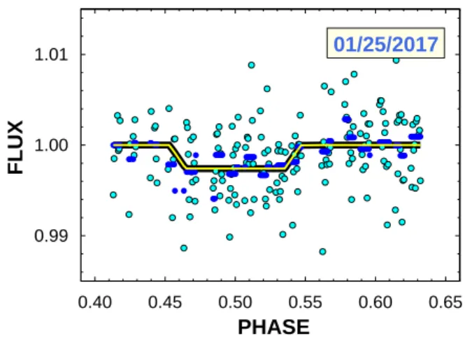
01/25/2017
Fig. A.3.Same as Fig.A.1, but for the night shown in the upper right corner.
with their statistical errors and some additional parameters are given in TableA.1. We note that the errors shown are unbiased because we considered the number of fitted parameters (Np) and the number of clipped data points (Nclip). All nightly occulta- tion values are within the 1σerror ranges, scattered around the merged value. Figures A.1–A.3 show the nightly data and the corresponding fits.