3. Soil moisture based drought monitoring by remote sensing and eld measurements
Boudewijn van Leeuwen; Károly Barta; Zsuzsanna Ladányi;
Viktória Blanka, György Sipos
Introduction
Drought is a phenomenon that can be characterised by an extended period of de - cient precipitation compared to the average and/or temperature that is much higher than the average, which consequently results in a signi cant water shortage (WMO and GWP, 2016). Several indices have been developed for the characterization of drought (e.g. Palmer, 1965; Pálfai, 2004, Balint et al., 2011, Zargar et al, 2011), which are mostly using the classic meteorological parameters (precipitation, temperature, etc.) and don’t take into account that the severity of drought is greatly in uenced by soil moisture conditions too. Some indices attempt to integrate this into the charac- terisation of drought in an indirect way, by utilising precipitation data for the period before the examined time frame – a good example of this the Pálfai Drought Index that is widely used in Hungary (Pálfai, 2004). Other indices already calculate with soil moisture, although the data are often not based on direct eld measurements, but applying simulated values (e.g. Narasimhan and Srinivasan, 2005). However, the role of soil moisture doesn’t only manifest in the regional modi cation of the drought’s severity, but also – depending on the soil types – in the spatial pattern of drought within a given region (country, region, area). For instance in Hungary and Serbia, in the arenosol areas situated in the Danube-Tisza Inter uves, the same meteorologi- cal situation results in much more severe drought than in the areas east of the Tisza River, characterized by chernozem soils. In Hungary water shortage can be calcu- lated for the upper 1 m layer of the soil from the simulation based soil moisture estimation of the National Meteorological Service (Chen and Dudhia, 2001; Horváth et al., 2015, OMSZ 2019a).
For on-site measurement of soil moisture several methods are available, and the most widespread methods worldwide and also in Hungary are based on dielec- tric constant measurement, especially the volumetric water content measurements utilising TDR (Time Domain Re ectometry) technology (Kirkham, 2014). Within the framework of a previous project (WAHASTRAT, HUSRB/1203/121/130; 2013-2014), 16 stations were installed in Southeast Hungary and in Vojvodina, where soil water content at six di erent depths (10, 20, 30, 45, 60 and 75 cm) and meteorological parameters are also measured (Barta et al., 2014). Based on the experiences of this
station network, a countrywide network of stations for meteorological and soil water content monitoring was installed in 2016 (Fiala et al., 2018), which is operated by the General Directorate of Water Management (OVF) and is expanded continuously. By the summer of 2019 the number of stations reached 47 (OVF Drought Monitoring 2019).
In spite of having an extensive monitoring system both horizontally and vertically, the preparation of nationwide map of the current soil moisture condition is also a major challenge, because the spatial extension of point type measurement data faces many di culties in the case of soil moisture. Just to mention a few: the spatial diversity of hydrophysical characteristics of soils (e.g. texture, saturated hydraulic conductivity, soil compaction), the role of macro- and microtopography in the devel- opment of moisture conditions, and the in uence of mosaic type land use and land coverage. Furthermore, on the site of monitoring stations, the agricultural cultiva- tion cannot be continued, therefore the di erence in land cover and the lack of soil cultivation question the representativeness of the measured soil moisture data at the stations. The solution to the complex problem can be the integration of remote sensing methods providing spatially continuous data.
Satellite remote sensing allows developing and applying algorithms that are capa- ble of deriving information from large area of the earth surface in a uniform method.
The estimation of soil moisture content based on satellite data has been a chal- lenge that was studied over the last 3 decades (Srivastava et al., 2016). Approaches based on data from optical, thermal infrared and microwave sensors have been applied to estimate soil moisture over large areas with a high temporal interval.
Barret and Petropoulos provide a detailed overview of these approaches (2014).
Most approaches to retrieve soil moisture from satellite data are nowadays based on microwave data. Especially with the launch of Sentinel 1 radar satellites this is a promising direction. Unfortunately, no medium to high resolution soil moisture product is available yet, and therefore in the research an optical – thermal infrared approach is followed.
The large spatial and temporal heterogeneity of soil moisture content makes it di cult make accurate estimates over large areas. Point measurements are repre- sentative for a relatively small area, while satellite-based measurements integrate measurements over a large area and store the result in one pixel. Calibration and validation of satellite-based measurements with eld measurements is therefore a di cult task.
In our research the aim is to provide continuous satellite derived soil moisture datasets for the project study area (Csongrád and Bács-Kiskun Counties in Hun- gary, Vojvodina in Serbia). To convert the resulted soil moisture index (SMI) maps to soil moisture content (SMC) in v/v% (volumetric water content, generally applied in pedology), the satellite derived SMI maps were attempted to be calibrated with eld measurements of the soil moisture content. This chapter describes the research methods and the gained experiences applied in the project.
Methods
The satellite data based approach presented here is based on MODIS vegetation index MOD13 16 day composites and MODIS land surface temperature MOD11 data. These data sets have been produced since 2000 and are therefore suitable for long term studies and continuous monitoring. The vegetation data is created by storing the maximum NDVI value for each pixel within a 16-day period (Huete 1999).
This way cloud and other disturbances are minimized and data for the total study area can be acquired. It is assumed that within the 16 day period the vegetation state is relatively stable. The spatial resolution of the data is 250 x 250 meter. The land surface temperature data is a daily product with a spatial resolution of 500 meter (Wang 1999). After registration, both input data sets can be downloaded and used freely.
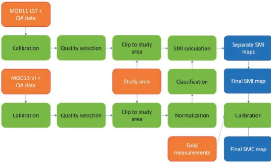
The optical – TIR based method is based on the assumption that thermal di er- ences in areas with similar vegetation cover are the result of changes in their soil moisture content (Vicente-Serrano et al., 2004). The algorithm was implemented using a set of python scripts and the arcpy geoprocessing library (Fig. 3.1).
Figure 3.1. Soil moisture index processing work ow
To determine areas with the similar vegetation cover, the NDVI layer is extracted from the MOD13 product. Using the reliability layer of the same MOD13 product, pixels with insu cient quality are removed. The remaining pixels are normalized and reclassi ed in 10 classes with equal width. Only if all classes are de ned (that have pixels), the algorithm is fully determined, and the temperatures are processed.
The land surface temperature layer is extracted from the MOD11 product. Only pixels with high quality are used for further processing. For each vegetation fraction
class, the minimum and maximum temperatures are extracted and the linear rela- tionship between the land surface temperature and soil moisture content index within the class is established using (1).
insufficient quality are removed. The remaining pixels are normalized
classes with equal width. Only if all classes are defined (that have pixels), the algorithm is fully determined, and the temperatures are processed. The land surface temperature layer is extracted from the MOD11 product. Only pixels with high quality are used for further processing. For each vegetation fraction class, the minimum and maximum temperatures are extracted and the linear relationship between the land surface temperature and soil moisture content index within the class is established using (1).
�
$,&=
()*()*+, -./()*+, 0 /()*+, -.
1 (1)
where SMI
i,cis the soil moisture index for pixel i in class c. In this way, 10 SMI maps are created giving the soil moisture content for each vegetation fraction class. Combining the separate SMI maps gives the final SMI map for the total study area. The final map contains index values between 0 (minimum soil moisture content) and 1 (maximum soil moisture content). SMI maps can only be determined if sufficient pixels are available in the vegetation and land surface data, and if every vegetation class is determined.
To convert the SMI maps to soil moisture content in v/v% units, the individual maps need to be calibrated with ground measurements. Two methods have been applied to calibrate the data. The first method is based on the soil moisture station network maintained by the Hungarian water authorities (OVF Aszálymonitoring 2019). This network consisted of 47 stations in March 2019 of which 27 are in the area that was covered by this study (Fig. 3.2).
Air temperature, soil moisture at 6 depths, soil temperature at 6 depths, relative humidity, and precipitation are measured by the stations. A php and curl API is provided to automatically download hourly data for every station. A python script was used to download the soil moisture data from a depth of 10 cm. For the period 01-01-2017 until 03-30-2019, if an SMI map was available, the soil moisture index was extracted from the SMI maps at the locations of the measurement stations, and compared to field measurements at 11:00 UTC, which is
(1)
where SMIi,c is the soil moisture indexfor pixel i in class c. In this way, 10 SMI maps are created giving the soil moisture content for each vegetation fraction class. Com- bining the separate SMI maps gives the nal SMI map for the total study area. The
nal map contains index values between 0 (minimum soil moisture content) and 1 (maximum soil moisture content). SMI maps can only be determined if su cient pixels are available in the vegetation and land surface data, and if every vegetation class is determined.
To convert the SMI maps to soil moisture content in v/v% units, the individual maps need to be calibrated with ground measurements. Two methods have been applied to calibrate the data. The rst method is based on the soil moisture station network maintained by the Hungarian water authorities (OVF Aszálymonitoring 2019). This network consisted of 47 stations in March 2019 of which 27 are in the area that was covered by this study (Fig. 3.2). Air temperature, soil moisture at 6 depths, soil temperature at 6 depths, relative humidity, and precipitation are measured by the stations. A php and curl API is provided to automatically download hourly data for every station. A python script was used to download the soil moisture data from a depth of 10 cm. For the period 01-01-2017 until 03-30-2019, if an SMI map was available, the soil moisture index was extracted from the SMI maps at the locations of the measurement stations, and compared to eld measurements at 11:00 UTC, which is more or less the time of the MODIS satellite overpass. In this way, for each day, the coe cient of determination between the satellite based measurements and the eld measurements was calculated. If the coe cient of determination was higher than 0.5, the original SMI map was calibrated using the slope and intercept derived from the eld measurements to get the nal SMC map.
Figure 3.2. Study area representing the soil moisture measurement stations and the eld measurement points obtained within the survey on 27 March 2019
The second calibration method was based on a eld measurement campaign exe- cuted on March 27, 2019. On that day, four teams measured soil moisture content in the eld using portable FieldScout TDR350 sensors (Fig. 3.3), which determine the average moisture of the soil’s upper 12 cm layer directly in v/v%, and with their integrated GPS module they instantly assign also the coordinates to the measure- ment points. Each team measured soil moisture at about 35 locations, over a route having a length of about 200 km per team (Fig. 3.2). Portable devices have made it possible to carry out a survey that represent the land use and soil type –of certain parts of the study area. During the selection of the measuring points, it was an important factor to select plots with a size that covers at least one full pixel in the remotely sensed MODIS images. Taking into account the 250 x 250 m resolution of
the images, the goal was to select minimum 500 x 500 m plots. Most of these were arable lands, but there were also grasslands, orchards (vineyards) and forests.
At the same locations of the eld measurements, soil moisture index data was extracted from the SMI map from the same day (Fig. 3.3). Also here, the coe cient of determination was calculated to evaluate the strength of the connection between the satellite derived estimates and the eld measurements.
Figure 3.3. Field measurement campaign on 27 March 2019 and the FieldScout TDR350 instrument
Resul ts
The satellite derived soil moisture maps were compared with the data of 27 soil moisture stations for the period 01/01/2017 until 29/03/2019. For 630 days a sat- ellite based SMI could be produced, but many maps were produced during cloudy days resulting in large areas without SMI values (Fig 3.4).
Figure 3.4 Soil moisture index maps with varying amount of missing data (gray areas) from 1 January 2017 (left), 25 April 2017 and 12 November 2018 (right)
To be able to determine the relation between the eld measurements and the sat- ellite data, it was decided that at least four points were required. In many cases, this requirement was not met, because the measurement stations were in areas where no SMI data was available. In total, on 440 days (or 70%), the regression equation could be determined. A further reduction was obtained because in many occasions the coe cient of determination was very low. It was decided that only if the rela- tionship was positive and the coe cient of determination was above 0.5, the data from the ground soil moisture station could be used to calibrate the SMI map. This resulted in 27 (or 7.5 % out of the total period of 630 days) SM maps (Fig 3.5).
Figure 3.5 Soil moisture content map, calibrated based on the soil moisture ground station network of the OVF for 14 July 2018.
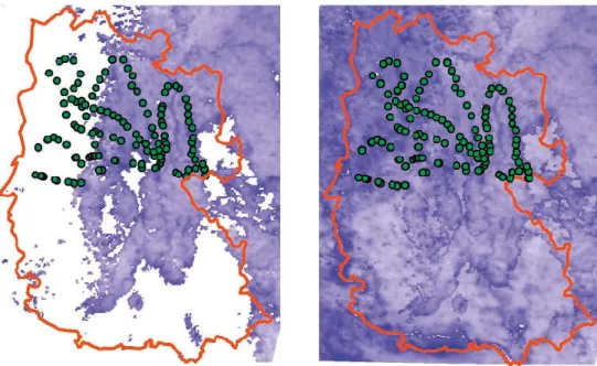
The soil moisture data measured on 27 March 2019, resulted in an in situ dataset of 136 soil moisture measurements. They were compared with the SMI map created based on satellite data for 28 March 2019. This was decided, because the image of the same day as the measurements was cloudy and in quite some places no data was available (Fig 3.6).
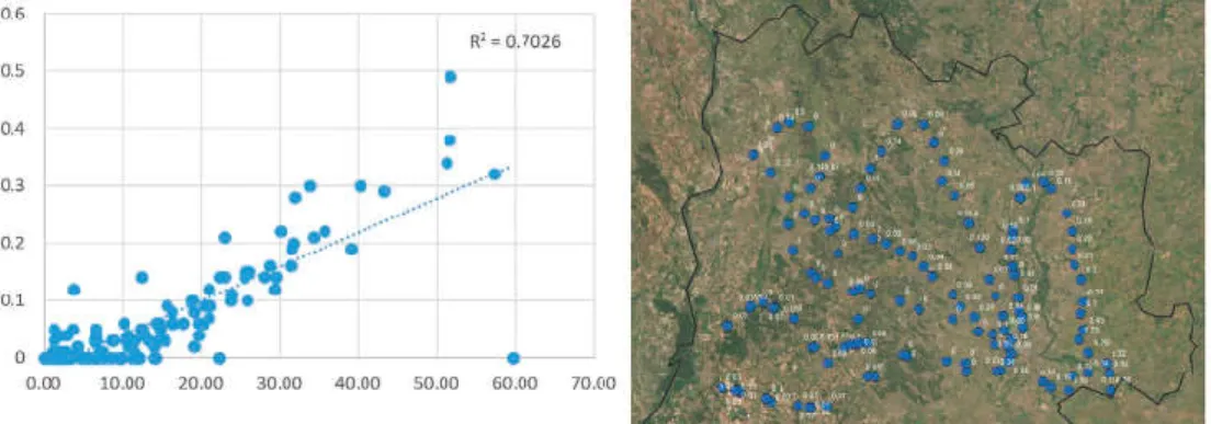
Based on the coordinates of each eld measurement, SMI data was extracted from the pixel that was located at the same location. These values were plotted against the soil moisture content values in the eld and the coe cient of determi- nation was calculated (Fig 3.7). Unfortunately, no statistical relationship between the values can be determined. Several attempts were made to create subsets for land use and soil type, but also then the coe cient of determination was close to 0.
Figure 3.6 Data availability for 27 March 2019 and 28 March 2019.
Figure 3.7 Relationship between volumetric soil moisture measurements in the eld (horizontal axis) and satellite derived soil moisture index values (vertical axis) (total data sets) The satellite derived soil moisture index values are indirectly derived from optical, near infrared and thermal data that measured over an area and integrated to one value for the complete pixel. The eld soil moisture measurements are point meas- urements representative for the direct surroundings of the measurement. The main reason for the lack of correspondence between the two data sets is this large di er- ence in scale. Another reason might be due to the fact that it is di cult to determine
which pixel in the satellite image represents the soil moisture index value at the location of the point measurement. Overlaying the two data sets shows that a point may be on the boundary of two pixels (Fig 3.8 upper left). When observing the loca- tion of the point measurements on a very high-resolution satellite image, it can be seen that the point probably represents the large eld to the south (Figure 8 upper right). To correct for this problem, this type of points was manually moved to the pixel that probably gave a more realistic value (Fig 3.8 lover left and lower right).
Unfortunately, also this manual correction did not provide a better coe cient of determination.
Figure 3.8 Manual adaptation of location of eld measurements to improve the SMI value extraction. Upper left: original location of the point measurement in yellow on top of the SMI map
(in gray). Upper right: original location of the point measurement on top of a very high resolution satellite image. Lower left: original point measurements (now in blue) were moved to their corrected
location (in yellow). Lower right: new point location on top of the SMI data
Another example of misrepresentation of the point measurements is given in Fig 3.9. The point measurement overlaid on the SMI le seems to represent one pixel, but in reality, that pixel is composed of an integrated soil moisture index value that is based on very di erent land cover types e.g. build up area, forest and elds with di erent types of agricultural activity (Fig 3.9 right).
Figure 3.9 Example of mixed land use
One of the most important requirements from the selected eld measurement points is to be located on a plots with homogenous land use, the size of which is bigger than twice the spatial resolution of the satellite image in both directions. Even on a homogenous plots, the di erences in temperature and moisture resulting from the microtopographic conditions can be problematic (Fig 3.8). Unfortunately in the study area, on both the arenosols with diverse relief and in the depressions and ridges of the slightly wavy Bácska Loess plateau, there are signi cant di erences in humus (in colour) and moisture content. In the measuring campaign, it could have been another source of error that the measuring was performed in a dry period, and the soil’s drying depth was 8-15 cm. This meant that the value measured by the 12 cm long sensor was the average of the dry upper soil layer and the wet layer below it. Our experience is that the best time for calibration is the period that begins 5-6 days after the end of a rainy period, when – depending on the hydrophysical characteristics of the soil – the drying of the soil has reached a stage that there are signi cant di erences between in both soil temperature and soil moisture, but the upper soil layer isn’t dry yet.
Another experience from the eld measurement campaign was that the meas- ured soil moisture data showed strong correlation with the soil’s salt content (Fig 3.10/a). Fig 3.10/b shows the spatial distribution of salt content, indicating that the salt content was much higher east of the Tisza River than in the Danube-Tisza inter uve. However, if those points where salt content is bigger than 0.06% were excluded and examine the relationship with only those soils that don’t have sodic soil characteristics, the correlation isn’t detectable. It can be concluded that the next measuring campaign, it would be useful to apply other soil moisture measurement types that are based on di erent methodology, too, for calibration purposes.
Figure 3.10 Relationship between soil moisture (VWC) and salt content (EC) in the study area (a), salt content values measured during the measuring campaign (b)
Conclusion
During the testing of the developed methodology, several limiting factors could be identi ed that make the applicability of calibration di cult. In the remaining period of the project a further measuring campaign is planned, based on the experiences, when the eld measurements will be carried out after a rainy period, so a wider spectrum of soil moisture data could be provided for calibration purposes, and more attention will be given to the pre-selection of larger and homogenous plots for measuring. Besides using the TDR technology portable devices, soil samples will also be collected to measure the water content (m/m%) of the soils also in the labo- ratory, by this eliminating the possible in uence of sodic soil characteristics. The SMI maps that are currently being created and published provide relative soil moisture data for the time being, which – although they don’t represent absolute volumetric percentage – are still capable of representing the actual spatial di erences in soil moisture conditions. In addition to the improving spatial resolution, radar data can be used to solve the problem of cloudy periods, but their calibration and validation issues still need to be resolved.