IDŐJÁRÁS Quarterly Journal of the Hungarian Meteorological Service

DOI:10.28974/idojaras.2019.3.7

IDŐJÁRÁS

Quarterly Journal of the Hungarian Meteorological Service Vol. 123, No. 3, July – September, 2019, pp. 371–390

Modeling of urban heat island using adjusted static database

Gergely Molnár^*, András Zénó Gyöngyösi, and Tamás Gál

Department of Climatology and Landscape Ecology, University of Szeged,

H-6722 Szeged, Egyetem u. 2., Hungary

*Corresponding author E-mail: molnarge@geo.u-szeged.hu (Manuscript received in final form June 26, 2018)

Abstract— In this study, the Weather Research and Forecasting (WRF) model was applied to examine the spatial and temporal formation of urban heat island (UHI) phenomenon in Szeged, Hungary. In order to achieve a more accurate representation of complex urban surface properties in WRF, a modified static database (consists of land use and urban canopy parameters) had been developed using satellite images and building information.

In the new database, the number of urban grids increased by 76% related to the default case. The urban landscape in WRF has become more complex after employing two urban land use classes instead of only one. The modification of the default parameters of a single layer urban scheme (i.e., Single Layer Urban Canopy Model – SLUCM) revealed that urban fractions decreased in all urban categories, while street widths increased resulting in narrower urban canyons. For testing the impact of the modifications on near-surface temperature estimation, a four-day heatwave period was selected from 2015. The model outputs had been evaluated against the observations of the local urban climate monitoring system (UCMS). WRF with the modified parameters simulated most of the features of UHI reasonably well. In most cases, biases with the simulations of the adjusted static database tended to be significantly lower than with the default parameters. Additionally, we picked out a longer time period (i.e., the summer of 2015) when the extreme values of near-surface air temperature and maxima of UHI intensities were evaluated on the basis of an urban and a rural site of UCMS. It was concluded that the maxima and minima of observed near- surface air temperature were underestimated (overestimated) by about 1–3 °C at the urban (rural) site. The maxima of UHI intensities indicated cold biases on 86 of 91 days.

Key-words: Weather Research and Forecasting model, Single Layer Urban Canopy Model, adjusted static database, urban heat island, Szeged (Hungary)

1.Introduction

Because of rapid urbanization since the 1850s, more than the half of Earth’s population live in cities nowadays, and estimations (UN, 2014) states that this ratio will likely to increase to 70% by the 2050s. The growing amount of artificial land cover alters the surface-atmosphere interaction of heat, moist, and momentum (Oke, 1973). Urban areas can be characterized by the urban heat island (UHI) phenomenon, which is a heat surplus related to rural regions (Oke, 1982).

UHI has been widely investigating recently, because climate change exacerbates this temperature anomaly (as a positive feedback) and also modifies urban bioclimatic conditions (Li and Bou-Zeid, 2013, IPCC, 2013). In addition to that, anthropogenic heat and pollutant release from industry, transportation, and residents gain energy consumption and medical expenditures (Crutzen, 2004, Kolokotroni et al., 2015). Monitoring of urban environment is mostly disposed by using in-situ measurements, satellite observations, and numerical meteorological models. Owing to a consecutive development of computer technology, application of numerical models comes with lower computational costs. The other obvious advantage of this method in contrast with in-situ measurements is that models can produce a nearly contiguous, high-resolution, three-dimensional meteorological field (Hidalgo et al., 2008). The quality and reliability of satellite products highly depend on atmospheric attenuation, which limits their application during the overpass time (Streutker, 2003). Contrarily, numerical simulations are not restricted by time and weather condition.

One of the major modeling challenges is to characterize complex urban surfaces (Mirzaei, 2015). It must be determined that whether a given land use grid (or a pixel on satellite images) is urban or non-urban, and if urban to which sub- category should be classified. In practice, the sub-categories consist of aerodynamic, thermodynamic, and geometric properties of the surface. The derivation of these parameters is troublesome, because the process requires a vast and accurate land surface information. In case of lack of such data, default values are used to give a “first guess” for the parameters, but this stipulation increases the uncertainty of simulations. It is also problematic that there is only a limited number of methods regarding the characterization of the complicated urban geometry.

A great effort was made by Stewart and Oke (2012) to address this issue with the Local Climate Zones (LCZs) scheme. LCZs aimed to define classes with a minimum extension of 200–400 m and analogous parameter-sets of geometric/surface cover (e.g., sky view factor, aspect ratio, building surface fraction, and terrain roughness class) and thermal/radiative/metabolic attributes (e.g., surface albedo and anthropogenic heat output). The categories were designated according to building type (from LCZ 1 to LCZ 10), land cover type (from LCZ A to LCZ G), and various land cover properties (from b to w). The World Urban Database and Portal Tool (WUDAPT) (Mills et al., 2015) project

has also been contributing to the global application and spread of urban climate modeling. Within this framework, a global, community land use database had been created utilizing the LCZ classification. Depending on complexity, the database of each city was separated into three levels. The lowest level (Level 0) includes LCZ maps with only a few parameters, while the others contain a more precise and detailed description of the measures. Recently (in April of 2018), the WUDAPT data is available to view for 21 European cities.

The Weather Research and Forecasting (WRF) numerical model has been employed in a wide range of applications, such as the simulation of UHI in specific cities (e.g., Sarkar and De Ridder, 2011, Salamanca et al., 2012, Giannaros et al., 2013), heatwave events (e.g., Li and Bou-Zeid, 2013, Wang et al., 2013, Chen at al., 2014), heavy rainfalls (e.g., Miao et al., 2011, Zhong and Yang, 2015), the impact of land use change on local climate (e.g., Pathirana et al., 2014, Brousse et al., 2016). Miao et al. (2009) investigated the behavior of urban heat island and boundary layer in Beijing. The results suggested that WRF coupled with the Single Layer Urban Canopy Model (SLUCM) scheme simulated reasonably well the spatial distribution and temporal variability of temperature field. Moreover, the model system captured the magnitude and direction of mountain-valley wind as well. Bhati and Mohat (2015) analyzed the impact of different land use categories on land surface temperature and near-surface air temperature in Delhi. The simulations were performed with (WRF-SLUCM) and without (WRF) the application of canopy parameterization scheme. By switching the SLUCM scheme on, RMSE of the land surface temperature decreased in urban grids (in non-urban grids) from 1.63 °C to 1.13 °C (from 2.89 °C to 2.75 °C). The hit rate of mean UHI enhanced by coupling WRF with SLUCM from 72% to 75%

in urban grids, from 65% to 73% in coastal grids, and from 52% to 71% in vegetation grids.

In Szeged, urban climate investigations have been typically based on in-situ (e.g., Unger et al., 2015) and mobile (e.g., Unger et al., 2001) measurements, but WRF was not used up to now. The study of Gál et al. (2016) must be pointed out, who evaluated a one-year long observation of the local urban climate monitoring system established in the spring of 2014. On average, UHI released around sunset and decreased to 0 °C after a few hours after sunrise. The maximum values of UHI arose generally three hours after sunset. The highest intensities culminated in LCZ 2, LCZ 3, and LCZ 5 in summer, with around 3.5 °C. The springtime means were just a little below 3 °C. On the other hand, the wintertime mean intensities remained only around 2 °C.

The specific aims of this study is i) to modify the default land use database and urban canopy parameter to allow a better representation for the surface geometry of Szeged, ii) to compare the spatial and temporal behavior of UHI with the default and adjusted dataset under anticyclonic weather condition, and iii) to evaluate the model performance during a longer time period using the observations of our local urban climate monitoring system.

2.Material and methods 2.1. Study area and urban climate monitoring system

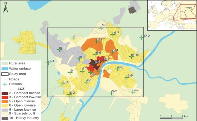
Szeged (46.26° N; 20.15° E) lies in the middle of the Hungarian Great Plain, at an elevation of 78–82 m AMSL, between sandy (to the west) and loamy (to the east) soil covered flat terrains. The Tisza River crosses the city, and several small- sized lakes are located to the northwest (Fig. 1), that may influence the local climate through evaporation cooling.

According to the Köppen-Geiger’s classification, Szeged is on the border of Cfb (marine temperate) and Dfb (humid continental) climates (Kottek et al., 2006), with an annual mean temperature of 10–12 °C and total precipitation of 500–600 mm. The dominance of high-pressure synoptic situation and local hot, dry wind blowing from the south in summer results in a high amount of annual sunshine duration (around 2000 hours).

With the population of 162,000, Szeged is the third largest city in Hungary.

Szeged has a concentric structure with radial avenues and several boulevards. The inner city accommodates offices, administrative and educational buildings, apartment houses. Towards outer parts, blocks of flats (mostly in the north- western part), family and gardening houses are found. At the outermost areas of Szeged, industrials, logistics, railway and highway junctions are located.

Fig. 1. Study area with the corresponding LCZs and urban climate monitoring sites.

An urban climate monitoring system (UCMS) has been established in the spring of 2014 within the framework of an EU project (URBAN-PATH Project, 2014, Lelovics et al., 2014). UCMS consists of 22 urban and two rural stations (Fig. 1.) and measures near-surface air temperature (with 0.2 °C accuracy between 10 °C and 60 °C) and humidity (with 1.8% accuracy between 10% and 90%) at the height of 4 m (Unger et al., 2015). Since urban canopy layer is well- mixed close to the surface, temperature measurements at this height are representative for lower layers as well (Nakamura and Oke, 1988). Until April of 2018, almost a four-year-long observation data is accessible for the evaluation of urban climate simulations, the model system, and further parameter fine-tuning purposes.

2.2. Modification of the land use database and specification of the SLUCM parameters

For accounting urban environment in numerical models, several urban canopy schemes have been created (Masson, 2000, Kusaka et al., 2001, Kusaka and Kimura, 2004, Martilli et al., 2002, Best et al., 2006, Oleson et al., 2008, Salamanca et al., 2010, Salamanca and Martilli, 2010). Here, we focused on the Single Layer Urban Canopy Model (SLUCM) of Kusaka et al. (2001), because other schemes (e.g., Building Energy Model (BEM) of Salamanca and Martilli (2010) require more complex parameters of anthropogenic activity in buildings (e.g., peak heat and heating profile generated by indoor equipment, etc.). SLUCM describes a ‘default’ city with a series of infinitely-long urban canyons where the effects of shadowing, reflection, and building orientation on short- and long-wave radiation are considered. Prognostic variables are skin temperature of wall, road and canopy, wind speed and direction at canopy level.

In order to achieve the best performance of a numerical weather prediction model, high-quality meteorological input, precise surface information (land use or soil data), physically consistent parameterization is needed. For representing the land use/land cover (LULC) of a given area, WRF offers the USGS (US Geological Survey) database (Homer et al., 2004) with a horizontal resolution of 30 m as an option. Over Europe, the CORINE (Coordination of Information on the Environment) data (Bossard et al., 2000) provides an alternate source of input static data with a horizontal resolution of 25 m. For the total study area, both databases largely underestimate the complexity of urban geometry, with only one urban category (Fig. 2). Therefore, we carried out a new LULC classification, based on the spectral features of urban grids, using eight Landsat 8 images. For non-urban grids, CORINE data was considered.

Fig. 2. USGS (a), CORINE (b), and modified (c) land use database at a model grid spacing of 2 km.

The Landsat 8 images (with a cloud fraction less than 3% for the entire scene) were merged into one false color composite to execute a maximum likelihood classification (Fig. 3). During the supervised classification, such small areas/clusters (region of interests; ROIs) were assigned (Fig. 3), that includes information about the size, location, and statistics of a given ROI representing LULC classes (i.e., commercial/industrial/transportation (CIT), low-intensity (LIR), and high-intensity residential (HIR)) in WRF.

Fig. 3. Methods utilized along the modification of land use (left panel) and SLUCM (right panel) databases.

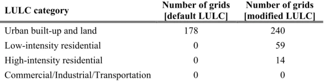
After the classification, it is concluded that 19% of the total urban (313) grids were categorized to LIR, 4% to HIR, and 0% to CIT, at a horizontal resolution of 2 km (Table 1 and Fig. 2).

Table 1. Number of urban grids in the default and the modified database according to LULC category

LULC category Number of grids

[default LULC]

Number of grids [modified LULC]

Urban built-up and land 178 240

Low-intensity residential 0 59

High-intensity residential 0 14

Commercial/Industrial/Transportation 0 0

WRF-SLUCM parameters (Kusaka et al., 2001; Kusaka and Kimura, 2004) tend to describe thermodynamic (e.g., wall, road, and roof albedo, heat capacities, and heat conductivities) and geometric (e.g., wall, road, and roof widths and heights, urban fraction) properties of an idealized urban canyon. Since default SLUCM values are not always suitable for any type of urban area, it is worth to modify these parameters if adequate surface information is available. In order to give a better representation of the surface elements in Szeged, we calculated some of the SLUCM parameters utilizing RapidEye satellite images and three- dimensional building database (containing building and roof height, building area and volume). First, the NDVI (normalized difference vegetation index) distribution of the satellite images was computed to separate water (NDVI < 0.0), built-up (0.0 ≤ NDVI ≤ 0.2), and vegetated (NDVI > 0.2) surfaces (Sobrino et al., 2004). In the following step, the building and NDVI databases were spatially joined to the three urban categories (Fig. 3). Assuming square-shaped urban canyons (on top-view), the road (Rx) and roof widths (rx) was predicted as follows:

x bx

x M

r = T ,

x ox x

x

M

T R N 1

=

where Tbx is the total building area, Tox is the total open area (difference of total area and total building area), Mx is the mean building height, and Nx is the number

of buildings (x refers to the corresponding urban LULC class). Aggregating and averaging the given parameters by urban categories, four new canopy parameters were achieved per LIR/HIR/CIT (Table 2).

Table 2. Modified and default (in parenthesis) urban canopy parameters applied to the study LULC category/canopy

parameter

Low-intensity residential

High-intensity residential

Commercial/Industrial/

Transportation

Building height [m] 6 (5) 6 (7.5) 6 (10)

Roof width [m] 5.5 (8.3) 5.5 (9.4) 6.2 (10)

Road width [m] 5.5 (8.3) 5.5 (9.4) 6.2 (10)

Urban fraction [-] 0.4 (0.5) 0.6 (0.9) 0.7 (0.95)

It was concluded that building height decreased (increased) to 6 m in HIR and CIT (LIR). Lower road and roof width (and building height) in each class resulted in a narrower urban canyon compared to the default case (in LIR the urban canyon is higher but also narrower), which may limit the shadowing effect (more energy on the surface) and enhance the reflection (trapping) of daytime incoming shortwave radiation and nocturnal outgoing long-wave radiation in the urban canyon. Consequently, simulated near-surface air temperatures may be higher in the daytime and lower in the nighttime as a result of the modification of canopy parameters. Urban fraction also decreased with an order between 10% and 30% (Table 2). Elevated evapotranspiration by lower urban fraction (and higher vegetation fraction) may counteract the potential warming during the daytime and strengthen the nocturnal cooling in the simulations. The rest of the default parameters have not been changed, because they fit to the local conditions or more suitable information were not obtained for further modifications.

3.Model setup

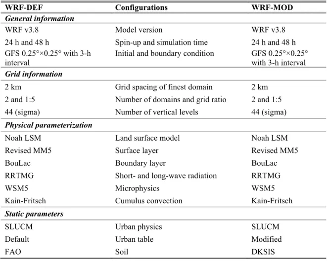
For testing the influence of the aforementioned modifications on near- surface air temperature (Ta) prediction over Szeged, we performed two types of model experiment with common grid and physical configurations but different static databases. Hereafter, simulations with the default (updated) land use and canopy parameters will be referred to as WRF-DEF (WRF-MOD) (Table 3).

WRF version 3.8. (Skamarock et al., 2008) had been used for each modeling purpose. Initial and boundary conditions were generated from the 0.25°×0.25°

resolution outputs of the Global Forecasting System (GFS) model at a three-hour interval. Parent domain (d01) employed a 10-km grid spacing, hosting a telescopic nest at 1:5 grid ratio resulting in a child domain (d02) with a final horizontal resolution of 2 km, with 96×96 grids centered over Szeged. 44 vertical sigma

levels were applied between the surface and 20 hPa. Physical parameterizations were chosen according to the applied urban scheme and above domain setup:

WSM 5-class scheme for microphysics (Hong et al., 2004), RRTMG scheme for long- and shortwave radiation (Iacono et al., 2008), MM5 Similarity scheme for surface layer (Jimenez et al., 2012), Unified Noah LSM (Tewari et al., 2004), BouLac scheme for boundary layer (Bougeault and Lacarrere, 1989), and Kain–

Fritsch scheme for cumulus convection (Kain, 2004), applied only for the parent domain.

Table 3. Model configuration and physical schemes applied to the modeling experiments

WRF-DEF Configurations WRF-MOD

General information

WRF v3.8 Model version WRF v3.8

24 h and 48 h Spin-up and simulation time 24 h and 48 h GFS 0.25°×0.25° with 3-h

interval

Initial and boundary condition GFS 0.25°×0.25°

with 3-h interval Grid information

2 km Grid spacing of finest domain 2 km

2 and 1:5 Number of domains and grid ratio 2 and 1:5

44 (sigma) Number of vertical levels 44 (sigma)

Physical parameterization

Noah LSM Land surface model Noah LSM

Revised MM5 Surface layer Revised MM5

BouLac Boundary layer BouLac

RRTMG Short- and long-wave radiation RRTMG

WSM5 Microphysics WSM5

Kain-Fritsch Cumulus convection Kain-Fritsch

Static parameters

SLUCM Urban physics SLUCM

Default Urban table Modified

FAO Soil DKSIS

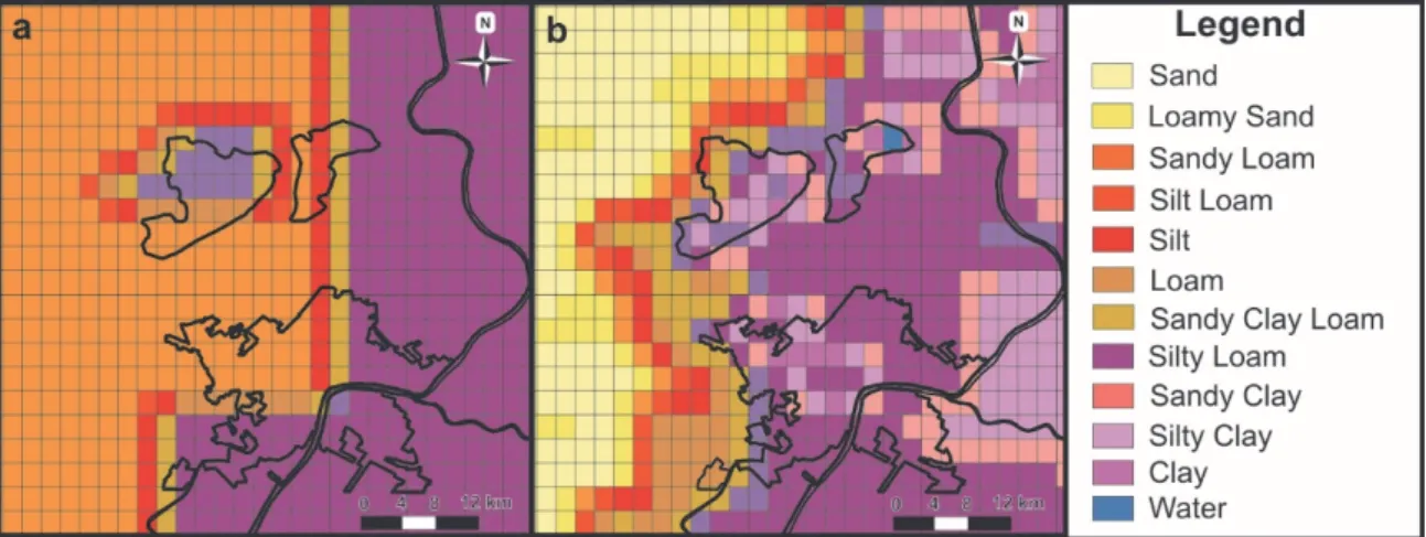
For representing soil texture in WRF-DEF, we employed the 16-category FAO (Food and Agriculture Organization) global database. To give a better characterization for the soil distribution in WRF-MOD, FAO was replaced to the DKSIS (Digital Kreybig Soil Information System) database (Pásztor et al., 2012) for those grids that located within the administrative border of Hungary (Fig 4).

Fig. 4. FAO (a) and DKSIS (b) soil databases at a model grid spacing of 2 km.

The integration of each day was initialized at 00 UTC and lasted for 48 hours.

The first 24 hours were dropped as spin-up, only the second half of the results (from 00 UTC to the next day's midnight) were considered and compared to the measurements under the verification process. The time-series of Ta at urban locations during their cooling stages showed a high-frequency noise of up to 3 °C amplitude. One-minute moving averages, however, induced pretty much reliable and low-biased results compared to the observations. For the reasons above, we performed a one-minute rolling average to the time-series of Ta.

The model output had been analyzed trough the UHI intensity parameter, which was defined as follows:

∆ = − ,

∆ = − ,

where ΔTOBS is the observed UHI intensity, TOBS x is the observed Ta at a given monitoring site, TOBS D-1 is the observed Ta at the D-1 reference rural station, ΔTWRF

is the modelled UHI intensity, TWRF x is the modeled Ta in the grid that located closest to the interested monitoring site, and TWRF D-1 is the modeled Ta in the grid that located closest to theD-1 reference rural station. For the evaluation, we selected time periods when urban effects were observed to be very well pronounced (ΔTOBS MAX >4.5 °C). Based upon the above criterion, four consecutive days between August 11 and August 14, 2015 was selected for the evaluation process of the two static datasets.

Once the standard model setup (WRF-MOD) was established, a series of background model integration was carried out for the whole period of the summer of 2015. On 48 days, the daily means of Ta ranged between 25–30 ºC, or even above 30 ºC on nine days in July and early August. Maxima were over 35 °C in 18 days in July and August. These heatwaves were characterized by high evening Ta and large

differences between urban and rural Ta. On the other hand, on 18 days daily means were under 20 ºC. Urban effect was completely missing or very weak during these periods. Otherwise, ΔTOBS were in most cases (on 56 nights) over 5 °C.

4. Results and discussion 4.1. Evaluation of the default and adjusted static dataset

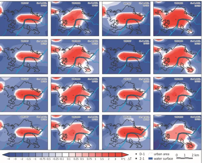
Both static databases had been verified against ΔTOBS of UCMS during the 4-day heatwave period. Fig. 5 represents the spatial distribution of ΔTWRF on each day at 03 UTC and 23 UTC, when this variable, on average, was observed to be the most intense. It is concluded that ΔTMAX with WRF-DEF was simulated to be 1–2 °C at 03 UTC and 2–3 °C at 23 UTC. Spatially, ΔTWRF correlated well with the distribution of USGS LULC data, and so it was limited to a small part of the city, with highest magnitudes over the northeast.

Fig. 5. Spatial distributions of ΔTWRF with WRF-DEF (A) and WRF-MOD (B) over Szeged between August 11 and 14, 2015 at 03 UTC (left side) and 23 UTC (right side). The black

ΔTWRF with WRF-MOD extended towards the outer areas, with peaks ranged from 2.5 °C to 4.5 °C. The tendency in ΔTWRF MAX between the two hours was not such straightforward in this case as previously: on the last two days, ΔTWRF was generally stronger at 03 UTC than at 23 UTC, by around 0.5 °C. ΔTWRF MAX was culminated along a southwest-northeast axis being reflected to the location of HIR classes (building fraction is 0.6). A more significant spatial variability of ΔTWRF, induced by the updated database, stemmed from the distinction of two urban categories (and two sets of canopy parameters) instead of using only the 'urban built-up and land' class to typify the sophisticated urban geometry.

Another remarkable peak (around 3 °C) was predicted over the south-eastern periphery of Szeged, particularly around 03 UTC. This obvious overestimation of ΔTOBS was the consequence of the horizontal resolution applied during the integration. Family houses and blocks of flats exist nearby, thus this area was classified to LIR. Those transition areas that lying near to the border of a given city are always difficult to threat on urban climate modeling, because they are characterized by urban and rural land cover features as well. Enhancing the horizontal resolution and introducing further LULC classes (e.g., LCZs) can be a potential way to avoid such inaccuracies.

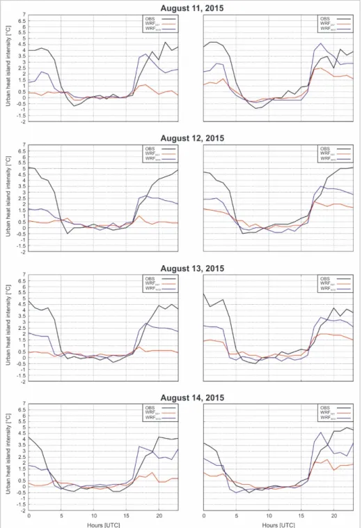
The mean diurnal variation of ΔTOBS andΔTWRF averaged according to LULC classes was illustrated in Fig. 6. The highest ΔTOBS MAX occurred in HIR on August 12 (around 5.5 °C), while the lowest was in LIR on August 14 (around 4 °C).

Overall, it was confirmed that the model, with WRF-MOD in particular, had the ability to estimate the daily fluctuation of ΔTOBS and to distinguish the evolution of ΔTOBS in different LULC. Regardless of the day of the simulation period, ΔTOBS

was approximated with lower accuracy in LIR, especially with WRF-DEF. On the other hand, biases with both parameter-sets decreased in HIR.

In the nighttime, ΔTOBS was mostly underestimated by the simulations of all datasets. With WRF-DEF, ΔTWRF remained around a constant value of 0.5–1 °C in LIR and showed only a moderate variability during the entire day. In HIR, the underestimation of ΔTOBS with WRF-DEF clearly decreased, especially in a couple of hours after sunset. The introduction of the new dataset decreased the uncertainties of nocturnal ΔTWRF with an order of 1–1.5 °C in LIR and 0.5 °C in LIR. In both urban categories, the underestimations simulated by WRF-MOD was shifted by an overestimation of 0.5–1 °C around sunset. The transition of nighttime to daytime ΔTOBS around sunrise (04 UTC) was captured properly in LIR and HIR as well. However, a slight time lag and faster balance of urban and rural Ta (i.e., faster decrease of ΔTWRF to 0 °C) existed.

The lower ΔTWRF in the nighttime could be the result of higher TWRF in the rural reference grid or lower TWRF in urban grids. In the next subsection it will be seen, that WRF generally underestimated TOBS over the urban area, thus ΔT was not being intensified by the simulation as by the observations. The substantial overestimations of ΔTOBS in WRF-MOD after sunset might be the consequence of an excessive energy income by the release of the formerly stored heat from artificial materials.

In the daytime, ΔTWRF with each of the two databases tended to be around 0 °C being in line with ΔTOBS of -0.5–0 °C. Therefore, no significant difference was given between WRF-DEF and WRF-MOD in neither LULC class at that time of the days. Otherwise, the magnitude of ΔTWRF was almost independent on the selection of the static parameters during the day.

Fig. 6. Mean diurnal variations of ΔTOBS and ΔTWRF with WRF-DEF and WRF-MOD in LIR (diagrams on the left) and HIR (diagrams on the right) LULC categories.

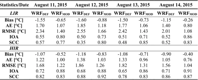
To analyze the accuracy of ΔTWRF with the different datasets on a statistic approach, the model outputs were compared with the observations through the daily means of bias, absolute error (AE), root mean squared error (RMSE), index of agreement (IOA), and spatial correlation coefficient (SCC) measures (Table 4).

Additionally, with the independent two-sample t-test, we investigated whether or not WRF-MOD was significantly enhanced the quality of the simulations.

As it was pointed out earlier, a robust underestimation of ΔTOBS occurred in each urban category. The biases (ΔTWRF-ΔTOBS) ranged from –1.60 °C to –0.26 °C.

The outputs of WRF decreased the corresponding errors, with around 0.8°C in LIR and 0.4 °C in HIR. AEs of ΔTWRF with WRF-MOD stayed below 1.18 °C, with the best performance on August 14 (around 0.75 °C). Even though WRF with each dataset performed similarly over the four days, some uncertainties still emerged on August 12 because of the less accurate initial field of GFS. In the future, it would be important to determine a threshold below which the erroneous data should be filtered out. Emery et al. (2001 employed a desired model accuracy of 0.8–1.0 for IOA. While WRF-DEF did not manage to exceed that limit, WRF- MOD, except on August 12 and 13 in LIR, fulfilled the expectations.

We performed the independent two-sample t-test at a confidence level of 0.95 and 0.99. The results suggested that ΔTWRF with WRF-MOD was estimated significantly better either in LIR or in HIR LULC categories, at a confidence of 95%. By increasing the confidence to 99%, the significance still persisted in LIR but not in HIR. Indeed, in HIR only a mean difference of 0.4 °C in ΔTWRF existed between the two datasets. In other words, the selection of the default static data does not generate larger uncertainties in a little part of the city (four HIR grids at 2 km horizontal resolution) under such conditions, although in the vast majority of the grids, the introduction of new parameters can contribute to a more efficient simulation of ΔT.

Table 4. Daily means of statistics of ΔTOBS and ΔTWRF (averaged for each day) with WRF- DEF and WRF-MOD in LIR and HIR LULC categories

Statistics/Date August 11, 2015 August 12, 2015 August 13, 2015 August 14, 2015 LIR WRFDEF WRFMOD WRFDEF WRFMOD WRFDEF WRFMOD WRFDEF WRFMOD

Bias [°C] -1.55 -0.65 -1.60 -0.88 -1.50 -0.73 -1.15 -0.26 AE [°C] 1.70 1.07 1.85 1.18 1.77 1.06 1.40 0.80 RMSE [°C] 2.34 1.40 2.55 1.66 2.42 1.43 2.01 1.08

IOA 0.55 0.80 0.50 0.73 0.51 0.71 0.52 0.86

SCC 0.57 0.77 0.35 0.80 0.48 0.85 0.52 0.83

HIR

Bias [°C] -1.07 -0.52 -1.18 -0.83 -1.08 -0.71 -0.90 -0.40 AE [°C] 1.22 1.00 1.38 1.03 1.33 0.96 1.05 0.76 RMSE [°C] 1.68 1.22 1.86 1.26 1.82 1.31 1.56 1.04

IOA 0.72 0.88 0.68 0.88 0.65 0.86 0.71 0.91

SCC 0.82 0.83 0.88 0.92 0.78 0.83 0.86 0.87

4.2. Analysis of the model performance with WRF-MOD

Through the detailed analysis of the measured data at all urban and rural locations (not shown here), it was found that the typical time variation of Ta at the 2–1 station represents the urban thermal conditions properly: compared to other time- series, this site was among the warmest ones at nights. Additionally, the station D-1 was still considered as rural station during the analysis. In this sub-section, we examined ΔTOBS and ΔTWRF based solely on TOBS and TWRF at these two stations.

The simulations were executed with the WRF-MOD configuration under a longer, 91-day period from June 1 to August 31, 2015. In order to validate the model results, we compared the mean and extreme values of TOBS 2-1, TOBS D-1, and ΔTOBS

to the corresponding TWRF 2-1, TWRF D-1, and ΔTWRF.

It can be seen in Fig 7 that the daily averages of TOBS, on average, were underestimated (overestimated) at the urban (rural) site by about 1.5 °C. Same can be stated for the TOBS MAX with slightly higher biases (around 2 °C). For TOBS MIN, a negative bias evolved at station 2–1 and a slight positive bias at station D-1. It must be noted that the underestimation of nocturnal TOBS over urban grids were also reported, for example, in the study of Bhati and Mohan (2015) and Kim et al.

(2013).

The daily ΔTOBS MAX was systematically underestimated on most of the days.

ΔTWRF MAX was higher than ΔTOBS MAX only in five cases. Negative biases in ΔTWRF

were even higher during the nights with a minimum of TOBS 2-1 >20 °C (warm nights in climate definition). It must be emphasized again that even if the magnitude of the ΔTWRF MAX had a systematic negative bias compared to the observations, the temporal variation was captured reasonably well.

If we concentrate on those days when both ΔTOBS MAX and ΔTWRF MAX (i.e., for example, around August 20) are low (i.e., less than 2.5 °C), it can be discovered that the minima of T2-1 and TD-1 was modeled with lower biases. On the other hand, large underestimations occurred in TOBS MAX at each station. At this time of the simulation period, a cut-off low pressure system dominated the Carpathian Basin causing a high degree of instability. This synoptic situation favored for daytime convective precipitation, which was not forecasted adequately by the model. Therefore, we intend to perform a data assimilation using the UCMS measurements and local radio sounding data of the Hungarian Meteorological Service. This time-consuming technique has been proven to be an efficient tool to predict most of the urban climate indicators (Liu et al., 2006 Tan et al., 2015).

Fig. 7. Maxima, means, and minima of ΔTOBS and ΔTWRF at a representative urban (station 2-1) and rural (station D-1) site of UCMS during the summer of 2015.

5.Conclusions and further plans

Using detailed city-specific built-up information and remote sensing data of Landsat 8 and RapidEye satellites, an adjusted static database (in terms of land use and urban canopy parameters; UCPs) had been created in order to better represent the physical characteristics of the urban forms in Szeged related to the default WRF dataset (WRF-DEF). In contrast with WRF-DEF, the modified land use dataset (WRF-MOD) consists of 76% more urban grids in the study area and employs two urban classes instead of only one at a model horizontal resolution of 2 km. After the calculation of canopy parameters, it was revealed that the urban canyons have become narrower, i.e., the parameters of building height, roof, and road width decreased related to WRF-DEF. Additionally, the building fraction also decreased from 90% (50%) to 60% (40%) in HIR (LIR). In turn, the vegetation fraction increased in both categories.

Following a predefined criterion (ΔTOBS MAX >4.5 °C), four days were selected to evaluate WRF with the above databases in simulating Ta. The model with WRF-MOD was able to capture the spatiotemporal variation of ΔTOBS

properly. On the other hand, the simulations with WRF-DEF contained large uncertainties. ΔTWRF with WRF-DEF restricted only to the downtown of Szeged, with maxima of around 2–3 °C. In WRF-MOD, ΔTWRF covered a much wider area of Szeged, with maxima (of around 4–4.5 °C) along a southwest-northeast axis located over the HIR LULC category. Some overestimations occurred near to the borders of the city, where a gradual transition of urban to rural surface is typical, that is really difficult to handle at such model resolution.

According to the observations of the local urban climate monitoring system, the highest ΔTOBS formed in HIR in a couple hours after sunset (18 UTC), with values of up to 5–5.5 °C. The nocturnal ΔTOBS was systematically underestimated, particularly in LIR. The biases decreased in HIR with the simulations of both static datasets. With WRF-MOD, slight overestimations occurred around sunset caused by the inaccurate timing of the nighttime heat release from artificial surface elements. ΔTWRF with WRF-DEF remained almost identical (0.5–1 °C) in LIR during the entire day. In the daytime, only a weak (0.5 °C) or even a negative (cool) (heat) island formed. Then ΔTWRF with either WRF-DEF or WRF-MOD was in line with the measurements in LIR and HIR as well.

Statistic scores of AE less than 1.18 °C with WRF-MOD indicated a good overall performance on ΔTOBS estimation. Moreover, the desired model accuracy of ΔT (IOA between 0.8 and 1.0) was mostly overachieved with ΔTWRF of WRF- MOD, except on August 12 and 13, in LIR. On the other hand, IOAs of WRF- DEF stayed always below 0.8. An independent two-sample t-test at a confidence level of 0.95 and 0.99 was performed to decide how much the introduction of the modified static database contributed to a better estimation of ΔTOBS during the 4-day heatwave event. It was concluded that ΔT with WRF-MOD was modeled significantly better (at both 95% and 99% confidence) in LIR than with WRF- DEF. In HIR, however, the significance was only valid at 95% confidence.

We analyzed the extreme values of TOBS, TWRF, ΔTOBS MAX, and ΔTWRF MAX based upon the observations and simulations (solely with WRF-MOD) of an urban (station 2–1) and rural (station D-1) site during the whole summer of 2015. TOBS MAX was underestimated (overestimated) by about 2 °C at the urban (rural) site. Similar tendencies were drawn out for TOBS MIN at both sites, with lower warm biases (around 1.5 °C), however, at station D-1. During this longer simulation period, ΔTOBS MAX was still underestimated (86 of 91 nights). If we considered those days when TOBS 2-1 >

20 °C, the biases of ΔTOBS MAX increased further on. Nonetheless, as we have seen earlier, the biases were generally within the acceptance limit, which implied an adequate quality of the simulations with WRF-MOD.

In order to improve our results and take the three-dimensionality of urban canopy into consideration even more accurately, we intend to test other urban parameterizations of WRF (i.e., BEM and BEP), with different parametrization schemes (for example, changing radiation, PBL, or LSM schemes) and domain setups (e.g., higher resolution). Inclusion of anthropogenic heat in the calculation and definition of further urban categories based on the LCZs may also contribute to better simulations. Furthermore, based on the high amount of measurements yielded by the unique urban temperature measurement network, we plan to assimilate the measured temperature data using three-dimensional variational technique.

Acknowledgements: This work was granted by the Hungarian Scientific Research Fund (OTKA K- 111768). The third author was supported by the ÚNKP-18-4 New National Excellence Program of the Ministry of Human Capacities.

References

Best, M.J., Grimmond, C.S.B., and Villani, M.G., 2006: Evaluation of the urban tile in MOSES using surface energy balance observations. Bound.-Layer Meteorol. 118, 503–525.

http://dx.doi.org/10.1007/s10546-005-9025-5

Bhati, S. and Mohan, M., 2015: WRF model evaluation for the urban heat island assessment under varying land use/land cover and reference site conditions. Theor. Appl. Climatol. 126, 385–400.

http://dx.doi.org/10.1007/s00704-015-1589-5

Bougeault, P. and Lacarrere, P., 1989: Parameterization of Orography–Induced Turbulence in a Mesobeta––Scale Model. Mon. Weather Rev. 117, 1872–1890.

http://dx.doi.org/10.1175/1520-0493(1989)117%3C1872:POOITI%3E2.0.CO;2

Bossard, M., Feranec, J., and Otahel, J., 2000: CORINE land cover technical guide. Addendum 2000.

Technical Report No. 40. Copenhagen: European Environmental Agency.

Brousse, O., Martilli, A., Foley, M., Mills, G., and Bechtel, B., 2016: WUDAPT, an efficient land use producing tool for mesoscale models? Integration of urban LCZ WRF over Madrid. Urb. Clim.

17, 116–134. http://dx.doi.org/10.1016/j.uclim.2016.04.001

Chen, F., Yang, X., and Zhu, W., 2014: WRF simulations of urban heat island under hot-weather synoptic conditions: The case study of Hangzhou City, China. Atmos. Res. 138, 364–377.

http://dx.doi.org/10.1016/j.atmosres.2013.12.005

Crutzen, P.J., 2004: New directions: The growing urban heat and pollution “island” effect-impact on chemistry and climate. Atmos. Environ. 38, 3539–3540.

http://dx.doi.org/10.1016/j.atmosenv.2004.03.032

Emery, C., Tai E., and Yardwood, G., 2001: Enhanced meteorological modeling and performance evaluation for two Texas ozone episodes. Environ. International Corporation.

Gál, T., Skarbit, N., and Unger, J., 2016: Urban heat island patterns and their dynamics based on an urban climate measurement network. Hun. Geo. Bull. 65, 105–116.

http://dx.doi.org/10.15201/hungeobull.65.2.2

Giannaros, T.M., Melas, D., Daglis, I.A., Keramitsoglou, I., and Kourtidis, K., 2013: Numerical study of the urban heat island over Athens (Greece) with the WRF model. Atmos. Environ. 73, 103–111.

http://dx.doi.org/10.1016/j.atmosenv.2013.02.055

Hidalgo, J., Masson, V., Baklanov, A., and Gimeno, L., 2008: Advances in urban climate modeling. Ann.

NY. Acad. Sci. 1146, 354–374. http://dx.doi.org/10.1196/annals.1446.015

Homer, C., Huang, C., Yang, L., Wylie, B., and Coan, M., 2004: Development of a 2001 national land cover database for the United States. Photogram. Eng. Rem. S. 70, 829–840.

http://dx.doi.org/10.14358/PERS.70.7.829

Hong, S.Y., Dudhia, J., and 0Chen, S.H., 2004: A revised approach to ice microphysical processes for the bulk parameterization of clouds and precipitation. Mon. Weather Rev. 132, 103–120.

http://dx.doi.org/10.1175/1520-0493(2004)132%3C0103:ARATIM%3E2.0.CO;2

Iacono, M.J., Delamere, J.S., Mlawer, E.J., Shephard, M.W., Clough, S.A., and Collins, W.D., 2008:

Radiative forcing by long- lived greenhouse gases: Calculations with the AER radiative transfer models. J. Geophys. Res. 113, D13103. http://dx.doi.org/10.1029/2008JD009944

IPCC, 2013: Climate Change 2013: The Physical Science Basis. Contribution of Working Group I to the Fifth Assessment Report of the Intergovernmental Panel on Climate Change (eds. Stocker, T.F., Qin, D., Plattner, G.K., Tignor, M., Allen, S.K., Boschung, J., Nauels, A., Xia, Y., Bex, V., Midgley, P.M.) Cambridge University Press, Cambridge, United Kingdom and New York, NY, USA.

Jimenez, P.A., Dudhia, J., Gonzalez–Rouco, J.F., Navarro, J., Montavez, J.P., and Garcia–Bustamante, E., 2012: A revised scheme for the WRF surface layer formulation. Mon. Weather Rev. 140, 898–918.

http://dx.doi.org/10.1175/MWR-D-11-00056.1

Kain, J.S., 2004: The Kain–Fritsch convective parameterization: An update. J. Appl. Meteor. 43, 170–

181. http://dx.doi.org/10.1175/1520-0450(2004)043%3C0170:TKCPAU%3E2.0.CO;2

Kim, Y., Sartelet, K., Raut, J.C., and Chazette, P., 2013: Evaluation of the Weather Research and Forecasting/Urban Model Over Greater Paris. Bound.-Layer Meteorol. 149, 105–132.

http://dx.doi.org/10.1007/s10546-013-9838-6

Kolokotroni, M., Ren, X., Davies, M., and Mavrogianni, A., 2015: London’s urban heat island: Impact on current and future energy consumption in office buildings. Energ. Buildings 47, 302–311.

http://dx.doi.org/10.1016/j.enbuild.2011.12.019

Kottek, M., Grieser, J., Beck, C., Rudolf, B., and Rubel, F., 2006: World map of the Köppen-Geiger climate classification update. Meteorol. Z. 15, 259–263.

Kusaka, H., Kondo, H., Kikegawa, Y., and Kimura, F., 2001: A simple single-layer urban canopy model for atmospheric models: Comparison with multi-layer and slab models. Bound.-Layer Meteorol.

101, 329–358. http://dx.doi.org/10.1023/A:1019207923078

Kusaka, H. and Kimura, F., 2004: Coupling a Single-Layer Urban Canopy Model with a Simple Atmospheric Model: Impact on Urban Heat Island Simulation for an Idealized Case. J. Meteorol.

Soc. Jpn. 82, 67–80. http://dx.doi.org/10.2151/jmsj.82.67

Lelovics, E., Unger, J., Gál, T., and Gál, C.V., 2014: Design of an urban monitoring network based on Local Climate Zone mapping and temperature pattern modelling. Clim. Res. 60, 51–62.

http://dx.doi.org/10.3354/cr01220

Li, D. and Bou-Zeid, E., 2013: Synergistic interactions between urban heat islands and heat waves: The impact in cities is larger than the sum of its parts. J. Appl. Meteorol. Clim. 52, 2051–2064.

http://dx.doi.org/10.1175/JAMC-D-13-02.1

Liu, Y., Chen, F., Warner, T., and Basara, J., 2006: Verification of a Mesoscale Data-Assimilation and Forecasting System for the Oklahoma City Area during the Joint Urban 2003 Field Project. J.

Appl. Meteor. Climatol. 45, 912–929. http://dx.doi.org/10.1175/JAM2383.1

Martilli, A., Clappier, A., and Rotach, M.W., 2002: An urban surface exchange parameterisation for mesoscale models. Bound.-Layer Meteorol. 104, 261–304.

http://dx.doi.org/10.1023/A:1016099921195

Masson, V., 2000: A Physically-Based Scheme For The Urban Energy Budget In Atmospheric Models.

Bound.-Layer Meteorol. 94, 357–397. http://dx.doi.org/10.1023/A:1002463829265

Miao, S., Chen, F., LeMone, M.A., Tewari, M., Li, Q., and Wang, Y., 2009: An observational and modeling study of characteristics of urban heat island and boundary layer structures in Beijing.

J. Appl. Meteor. Climatol. 48, 484–501. http://dx.doi.org/10.1175/2008JAMC1909.1

Miao, S., Chen, F., Li, Q., and Fan, S., 2011: Impacts of urban processes and urbanization on summer precipitation: A case study of heavy rainfall in Beijing on 1 August 2006. J. Appl. Meteorol.

Climatol. 50, 806–825. http://dx.doi.org/10.1175/2010JAMC2513.1

Mills, G., Bechtel, B., Ching, J., See, L., Feddema, J., Foley, M., Alexander, P., and O’Connor, M., 2015: An introduction to the WUDAPT project. Proceedings of the ICUC9. Meteo France, Toulouse, France.

Mirzaei, P.A., 2015: Recent challenges in modeling of urban environment. Sust. Cit. Soc. 19, 200–206.

https://doi.org/10.1016/j.scs.2015.04.001

Nakamura, Y. and Oke, T.R., 1988: Wind, temperature and stability conditions in an east-west oriented urban canyon. Atmos. Environ. 22, 2691–2700. http://dx.doi.org/10.1016/0004-6981(88)90437-4 Oke, T.R., 1973: City size and the urban heat island. Atmos. Environ. 7, 769–779.

http://dx.doi.org/10.1016/0004-6981(73)90140-6

Oke, T.R., 1982: The energetic basis of urban heat island. Q. J. Roy. Meteor. Soc. 108, 1–24.

http://dx.doi.org/10.1002/qj.49710845502

Oleson, K.W., Bonan, G.B., Feddema, J., Vertenstein, M., and Grimmond, C.S.B., 2008: An urban parameterization for a global climate model. Part 1: Formulation and evaluation for two cities. J.

Appl. Meteor. Climat. 47, 1038–1060. http://dx.doi.org/10.1175/2007JAMC1597.1

Pathirana, A., Denekew, H.B., Veerbeek, W., Zevenbergen, C., and Banda, A.T., 2014: Impact of urban growth-driven landuse change on microclimate and extreme precipitation – A sensitivity study.

Atmos. Res. 138, 59–72. http://dx.doi.org/10.1016/j.atmosres.2013.10.005

Pásztor, L., Szabó, J., Bakacsi, Zs., Matus, J., and Laborczi, A., 2012: Compilation of 1:50,000 scale digital soil maps for Hungary based on the digital Kreybig soil information system. J. Maps 8, 215–219. https://doi.org/10.1080/17445647.2012.705517

Salamanca, F., Krpo, A., Martilli, A., and Clappier, A., 2010: A new building energy model coupled with an urban canopy parameterization for urban climate simulations–part I. formulation, verification, and sensitivity analysis of the model. Theor. Appl. Climatol. 99, 331–344.

Salamanca, F. and Martilli, A., 2010: A new building energy model coupled with an urban canopy parameterization for urban climate simulations–part II. Validation with one dimension offline simulations. Theor. Appl. Climatol. 99, 345–356. http://dx.doi.org/10.1007/s00704-009-0143-8 Salamanca, F., Martilli, A., and Yagüe, C., 2012: A numerical study of the Urban Heat Island over

Madrid during the DESIREX (2008) campaign with WRF and an evaluation of simple mitigation strategies. Int. J. Climatol. 32, 2372–2386. http://dx.doi.org/10.1002/joc.3398

Sarkar, A. and De Ridder, K., 2011: The urban heat island intensity of Paris: A case study based on a simple urban surface parametrization. Bound. Lay. Meteorol. 138, 511–520.

http://dx.doi.org/10.1007/s10546-010-9568-y

Skamarock, W.C., Klemp, J.B., Dudhia, J., Gill, D.O., Barker, D.M., Duda, M.G., Huang, X.Y., Wang, W., and Powers, J.G., 2008: A Description of the Advanced Research WRF Version 3. NCAR Tech. Note NCAR/TN-475+STR, 113 p. http://dx.doi.org/10.5065/D68S4MVH.

Sobrino, J.A., Jimenez-Munoz, J.C., and Paolini, L., 2004: Land surface retrieval from Landsat 5 TM.

Rem. S. Environ. 90, 434–440. https://doi.org/10.1016/j.rse.2004.02.003

Stewart, I.D. and Oke, T.R., 2012: Local Climate Zones for urban temperature studies. Bull. Amer.

Meteor. Soc. 93, 1879−1900. http://dx.doi.org/10.1175/BAMS-D-11-00019.1

Streutker, D.R., 2003: Satellite-measured growth of the urban heat island of Houston. Texas. Rem. Sens.

Environ. 85, 282–289. http://dx.doi.org/10.1016/S0034-4257(03)00007-5

Tan, J., Yang, L., Grimmond, C.S., Shi, J., Gu, W., Chang, Y., Hu, P., Sun, J., Ao, X., and Han, Z., 2015: Urban Integrated Meteorological Observations: Practice and Experience in Shanghai, China. Bull. Amer. Meteor. Soc. 96, 85–102. https://doi.org/10.1175/BAMS-D-13-00216.1 Tewari, M., Chen, F., Wang, W., Dudhia, J., LeMone, M.A., Mitchell, K., Ek, M., Gayno, G., Wegiel, J.,

and Cuenca, R.H., 2004: Implementation and verification of the unified NOAH land surface model in the WRF model. 20th conference on weather analysis and forecasting/16th conference on numerical weather prediction, 11–15.

Unger, J., Sümeghy, Z., Gulyás, Á., Bottyán, Zs., and Mucsi, L., 2001: Land-use and meteorological aspects of the urban heat island. Meteorol. Appl. 8, 189–194.

http://dx.doi.org/10.1017/S1350482701002067

Unger, J., Gál, T., Csépe, Z., Lelovics, E., and Gulyás, Á., 2015: Development, data processing and preliminary results of an urban human comfort monitoring and information system. Időjárás 119, 337–354.

United Nations, 2014: World Urbanization Prospects: The 2014 Revision. Department of Economic and Social Affairs, Population Division, 32 p.

URBAN-PATH Project, 2014: Evaluations and public display of urban patterns of human thermal conditions. http://urban-path.hu/

Wang, M., Yan, X., Liu, J., and Zhang, X., 2013: The contribution of urbanization to recent extreme heat events and potential mitigation strategy in the Beijing–Tianjin–Hebei metropolitan area. Theor.

Appl. Climatol. 114, 407–416. http://dx.doi.org/10.1007/s00704-013-0852-x

Zhong, S. and Yang, X.Q., 2015: Ensemble simulations of the urban effect on a summer rainfall event in the Great Beijing Metropolitan Area. Atmos. Res. 153, 318–334.

http://dx.doi.org/10.1016/j.atmosres.2014.09.005