Data mining

(1)

G Á B O R B E R E N D

D ATA M I N I N G

(2)

and supported by the European Union. Project identity number:

EFOP-3.4.3-16-2016-00014

(3)

T ^{ABLE OF} C ^ONTENTS

1 About this book 15

1.1 How to Use this Book 15

2 Programming background 17

2.1 Octave 17 2.2 Plotting 26

2.3 A brief comparison of Octave and numpy 29 2.4 Summary of the chapter 30

3 Basic concepts 31

3.1 Goal of data mining 32 3.2 Representing data 38

3.3 Information theory and its application in data mining 46 3.4 Eigenvectors and eigenvalues 50

3.5 Summary of the chapter 54

4 Distances and similarities 55

4.1 Minkowski distance 57

4.2 Mahalanobis distance 60

4.3 Cosine distance 62

4.4 Jaccard similarity 64

4.5 Edit distance 66

(4)

4.8 Summary of the chapter 75

5 Finding Similar Objects Efficiently 76

5.1 Locality Sensitive Hashing 76

5.2 Approaches disallowing false negatives 90 5.3 Summary of the chapter 99

6 Dimensionality reduction 100

6.1 The curse of dimensionality 101 6.2 Principal Component Analysis 105 6.3 Singular Value Decomposition 118 6.4 Linear Discriminant Analysis 131 6.5 Further reading 135

6.6 Summary of the chapter 137

7 Mining frequent item sets 138

7.1 Important concepts and notation for frequent pattern mining 139 7.2 Apriori algorithm 146

7.3 Park–Chen–Yu algorithm 155 7.4 FP–Growth 159

7.5 Summary of the chapter 166

8 Data mining from networks 168

8.1 Graphs as complex networks 168 8.2 Markov processes 171

8.3 PageRank algorithm 177 8.4 Hubs and Authorities 186 8.5 Further reading 189

8.6 Summary of the chapter 190

4

(5)

9 Clustering 191

9.1 What is clustering? 191 9.2 Agglomerative clustering 193 9.3 Partitioning clustering 200 9.4 Further reading 208

9.5 Summary of the chapter 209

10 Conclusion 210

A Appendix — Course information 211 Bibliography 215

5

(6)

2.1 A screenshot from the graphical interface of Octave. 18 2.2 Code snippet:Hello world! in Octave 19

2.3 Code snippet: An example for using a for loop and conditional execution with an if construction to print even numbers between1and 10. 19

2.4 Code snippet: The general syntax for defining a function 20 2.5 Code snippet: A simple function receiving two matrices and return-

ing both their sum and difference. 20

2.6 Code snippet: An example of a simple anonymous function which returns the squared sum of its arguments (assumed to be scalars instead of vectors). 21

2.7 Code snippet: An illustration of indexing matrices in Octave. 22 2.8 Code snippet: Centering the dataset withforloop 23

2.9 Code snippet: Centering the dataset relying on broadcasting 23 2.10Code snippet: Calculating the columnwise sum of a matrix with a

forloop. 24

2.11Code snippet: Calculating the columnwise sum of a matrix in a vectorized fashionwithoutaforloop. 25

2.12Code snippet: Calculating the columnwise sum of a matrix in a semi- vectorized fashion with single aforloop. 25

2.13Code snippet: Transforming vectors in a matrix to unit-norm by relying on aforloop. 26

2.14Code snippet: Transforming vectors in a matrix to unit-norm in a vectorized fashionwithoutaforloop. 26

2.15Code snippet: Code for drawing a simple function f x 2x³over the range 3, 4 . 26

2.16The resulting output of the code snippet in Figure2.15for plotting the function f x 2x³over the interval 3, 4 . 27

2.17Code snippet: Code for drawing a scatter plot of the heights of the people from the sample to be found in Table2.1. 27

2.18Scatter plot of the heights and weights of the people from the sample to be found in Table2.1. 28

(7)

2.19Code snippet: Code for drawing a histogram of the heights of the people from the sample to be found in Table2.1. 28

2.20Histogram of the heights of the people from the sample to be found in Table2.1. 28

2.21Code snippet: Comparing matrix-style and elementwise muliplication of matrices. 29

3.1 The process of knowledge discovery 33

3.2 Example of a spurious correlation. Source: http://www.tylervigen.

com/spurious-correlations 33

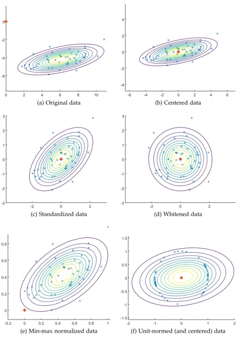
3.3 Code snippet: Various preprocessing steps of a bivariate dataset 41 3.4 Various transformations of the originally not origin centered and cor-

related dataset (with the thick orange cross as the origin). 42 3.5 Math Review: Scatter and covariance matrix 44

3.6 Math Review: Cholesky decomposition 45 3.7 Math Review: Shannon entropy 46

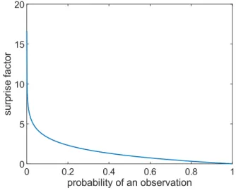
3.8 The amount of surprise for some event as a function of the probability of the event. 47

3.9 Sample feature distribution with observations belonging into two possible classes (indicated by blue and red). 49

3.10Code snippet: Eigencalculation using Octave 53

3.11Code snippet: An alternative way of determining the eigenpairs of matrixMwithout relying on the built-in Octave function^eig. 53

4.1 Illustration for the symmetric set difference fulfilling the triangle inequality. 57

4.2 Unit circles with for variouspnorms. 58 4.3 Example points. 59

4.4 Motivation for the Mahalanobis 60

4.5 Illustration of the Mahalanobis distance. 61 4.6 Illustration of the cosine distance 62 4.7 Math Review: Law of cosine 63 4.8 An example pair of setsXandY. 65

4.9 The visualization of the Bhattacharyya coefficient for a pair of Bernoulli distributionsPandQ. 69

4.10Illustration for the Bhattacharyya distance not obeying the property of triangle inequality. 70

4.11Illustration for the Hellinger distance for the distributions from Ex- ample4.7. 71

4.12Visualization of the distributions regarding the spare time activities in Example4.8. R, C and H along the x-axis refers to the activities reading, going to the cinema and hiking, respectively. 73 4.13Code snippet: Sample code to calculate the difference distance/di-

vergence values for the distributions from Example4.8. 74

7

(8)

matrix 78

5.3 Code snippet: Determine the minhash function for the characteris- tic matrix 78

5.4 Code snippet: Determine the minhash function for the characteris- tic matrix 81

5.5 Illustration of Locality Sensitive Hashing. The two bands colored red indicates that the minhash for those bands are element-wise identical. 83

5.6 Illustration of the effects of choosing different band and row number during Locality Sensitive Hashing for the Jaccard distance. Each subfigure has the number of rows per band fixed to one of 1, 3, 5, 7 and the values forbrange in the interval 1, 10 . 84

5.7 The ideal behavior of our hash function with respect its probability for assigning objects to the same bucket, if our threshold of critical similarity is set to 0.6. 85

5.8 The probability of assigning a pair of objects to the same basket with different number of bands and rows per bands. 85

5.9 The probability curves when performing AND-construction (r 3) followed by OR-constructions (b 4). The curves differ in the order the AND,-and OR-constructions follow each other. 87 5.10Code snippet: Illustration of combining AND/OR-amplifications in

different order. 87

5.11Math Review: Dot product 88

5.12Illustration of the geometric probability defined in Eq. (5.7). Randomly drawn hyperplaness₁ands2are denoted by dashed lines. The range of the separating angle and one such hyperplane (s1) is drawn in red, whereas the non-separating range of angle and one such hyperplane (s2) are in blue. 89

5.13Approximation of the angle enclosed by the two vectors as a function of the random projections employed. The value of the actual angle is represented by the horizontal line. 90

5.14Math Review: Euler’s constant 96

5.15Illustration of the Euler coefficient as a limit of the sequence 1 ¹_n ⁿ. 97 5.16False positive rates of a bloom filter with different load factors as a

function of the hash functions employed per inserted instances. The different load factors corresponds to different average number of objects per a bucket (G/m). 98

6.1 Gamma function over the interval [0.01,6] with integer values denoted with orange crosses. 101

6.2 Math Review: Gamma function 102

8

(9)

6.3 The volume of a unit hypersphere as a function of the dimension- alityd. 102

6.4 The relative volume of the 1 sphere to the unit sphere. 103 6.5 The position of a (red) hypersphere which touches the (blue) hyper-

spheres with radius1. 103

6.6 The radius of the hypersphere inddimensions which touches the 2^dnon-intersecting unit hyperspheres located in a hypercube with sides of length4. 104

6.7 The distribution of the pairwise distances between1000pairs of points in different dimensional spaces. 105

6.8 Math Review: Constrained optimization 108

6.9 An illustration of the solution of the constrained minimization prob- lem for f x,y 12x 9ywith the constraint that the solution has to lie on the unit circle. 109

6.10Math Review: Eigenvalues of scatter and covariance matrices 111 6.11Code snippet: Calculating the1–dimensional PCA representation of

the data set stored in matrix M. 112

6.12A25element sample from the5,000face images in the data set. 113 6.13Differently ranked eigenfaces reflecting the decreasing quality of eigen-

vectors as their corresponding eigenvalues decrease. 114

6.14Visualizing the amount of distortion when relying on different amount of top-ranked eigenvectors. 115

6.15Math Review: Eigendecomposition 119 6.16Math Review: Frobenius norm 120

6.17Code snippet: Performing eigendecomposition of a diagonalizable matrix in Octave 121

6.18Visual representation of the user rating data set from Table6.2in3D space. 123

6.19The reconstructed movie rating data set based on different amount of singular vectors. 125

6.20Code snippet: An illustration that the squared sum of singular values equals the squared Frobenius norm of a matrix. 126

6.21The latent concept space representations of users and movies. 128 6.22Example data set for CUR factorization. The last row/column includes

the probabilities for sampling the particular vector. 130 6.23An illustration of a tensor. 131

6.24An illustration of the effect of optimizing the joint fractional objec-

tive of LDA (b) and its nominator (c) and denominator (d) separately. 134 6.25Code snippet: Code snippet demonstrating the procedure of LDA. 135 6.26Illustration of the effectiveness of locally linear embedding when ap-

plied on a non-linear data set originating from an S-shaped mani- fold. 136

9

(10)

7.2 Illustration of the distinct potential association rules as a function of the different items/features in our dataset (d). 144

7.3 The relation of frequent item sets to closed and maximal frequent item sets. 146

7.4 Code snippet: Performing counting of single items for the first pass of the Apriori algorithm. 154

7.5 Code snippet: Performing counting of single items for the first pass of the Park-Chen-Yu algorithm. 158

7.6 The FP-tree over processing the first five baskets from the example transactional dataset from Table7.7. The red dashed links illustrate the pointers connecting the same items for efficient aggregation. 163 7.7 FP-trees obtained after processing the entire sample transactional database

from Table7.7when applying different item ordering. Notice that the pointers between the same items are not included for better vis- ibility. 164

7.8 FP-trees conditionated on item set{E}with different ordering of the items applied. 165

8.1 A sample directed graph with four vertices (a) and its potential representations as an adjacency matrix (b) and an edge list (c). 170 8.2 Code snippet: Creating a dense and a sparse representation for the

example digraph from Figure8.1. 170

8.3 Math Review: Eigenvalues of stochastic matrices 172

8.4 An illustration of the Markov chain given by the transition probabilities from8.2. The radii of the nodes – corresponding to the different states of our Markov chain – if proportional to their stationary distribution. 176

8.5 Code snippet: The uniqueness of the stationary distribution and its global convergence property is illustrated by the fact that all5ran- dom initializations forpconverged to a very similar distribution. 176 8.6 An example network and its corresponding state transition matrix. 179 8.7 An example network which is not irreducible with its state transi-

tion matrix. The problematic part of the state transition matrix is in red. 181

8.8 An example network which is not aperiodic with its state transition matrix. The problematic part of the state transition matrix is in red. 182 8.9 An example (non-ergodic) network in which we perform restarts fa-

voring state1and2(indicated by red background). 185 8.10Example network to perform HITS algorithm on. 189

9.1 A schematic illustration of clustering. 192

10

(11)

9.2 Illustration of the hierarchical cluster structure found for the data points from Table9.1. 197

9.3 An illustration of the k-means algorithm on a sample dataset with k 3 with the trajectory of the centroids being marked at the end of different iterations. 203

9.4 Using k-means clustering over the example Braille dataset from Fig- ure9.1. Ideal clusters are indicated by grey rectangles. 204 9.5 Math Review: Variance as a difference of expectations 207

11

(12)

2.1 Example dataset containing height and weight measurements of people. 27

3.1 Example dataset illustrating Simpson’s paradox 34

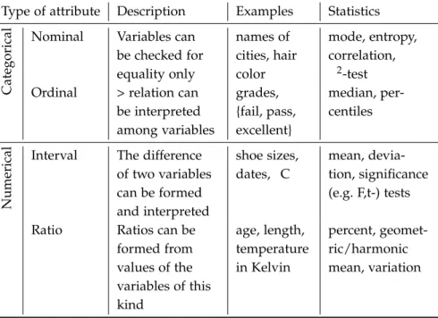
3.2 Typical naming conventions for the rows and columns of datasets. 38 3.3 Overview of the different measurement scales. 38

3.4 Illustration of the possible treatment of a nominal attribute. The newly introduced capitalized columns correspond to binary features indicating whether the given instance belongs to the given nationality, e.g., whenever the BRA variable is1, the given object is Brazilian. 40 3.5 An example contingency table for two variables. 47

3.6 Sample data set for illustrating feature discretization using mutual information. 50

4.1 Various distances between the distribution regarding Jack’s leisure activities and his colleagues. The smaller values for each notions of distances is highlighted in bold. 73

5.1 Step-by-step derivation of the calculation of minhash values for a fixed permutation. 80

6.1 Example user-item data set with a lower than observed effective dimensionality. 105

6.2 Example rating matrix data set. 122

6.3 The cosine similarities between the2-dimensional latent representations of user Anna and the other users. 127

6.4 The predicted rating given by Anna to the individual movies based on the top-2singular vectors of the rating matrix. 127

6.5 The values of the different components of the LDA objective (along the columns) assuming that we are optimizing towards certain parts of the objective (indicated at the beginning of the rows). Best values along each column are marked bold. 135

7.1 Example transactional dataset. 139

(13)

7.2 Compressing frequent item sets — Example (t =3) 147

7.3 Sample transactional dataset (a) and its explicit and its corresponding incidence matrix representation (b). The incidence matrix con- tains1for such combinations of baskets and items for which the item is included in the particular basket. 153

7.4 The upper triangular of the table lists virtual item pair identifiers obtained by the hash functionh x,y 5 x y 3 mod 7 1 for the sample transactional data set from Table7.3. The lower triangular values are the actual supports of all the item pairs, with the values in the diagonal (in parenthesis) include supports for item sin- gletons. 157

7.5 The values stored in the counters created during the first pass of the Park-Chen-Yu algorithm over the sample transactional dataset from Table7.3. 157

7.6 Support values forC2calculated by the end of the second pass of PCY. 159 7.7 Example market basket database. 162

7.8 The transactional dataset indicating irrelevant transactions with respect item set{E}. Irrelevant baskets are striked. 165

8.1 The convergence of the PageRank values for the example network

from Figure8.6. Each row corresponds to a vertex from the network. 180 8.2 Illustration of the power iteration for the periodic network from Fig-

ure8.8. The cycle (consisting of a single vertex) accumulates all the importance within the network. 183

8.3 The probability of restarting a random walk after varying number of steps and damping factor . 184

8.4 Illustration of the power iteration for the periodic network from Fig- ure8.8when a damping factor 0.8 is applied. 184

8.5 Illustration of the convergence of the HITS algorithm for the example network included in Figure8.10. Each row corresponds to a vertex from the network. 189

9.1 Example2-dimensional clustering dataset. 196

9.2 Pairwise cluster distances during the execution of hierarchical clustering. The upper and lower triangular of the matrix includes the between cluster distances obtained when using complete linkage and single linkage, respectively. Boxed distances indicate the pair of clusters that get merged in a particular step of hierarchical clustering. 197 9.3 Illustration of the calculation of the medoid of a cluster. 198

9.4 An example where matrix of within-cluster distances for which different ways of aggregation yields different medoids. 199 9.5 Calculations involved in the determination of biased sample vari-

ance in two different ways for the observations 3, 5, 3, 1 . 207

13

(14)

9.7 Illustration of the BFR representations of clustersC1 A,B,C andC2 D,E for the data points from Table9.6. 209

14

(15)

1 | A BOUT THIS BOOK

This book was primarily written as a teaching material for computer science students at the University of Szeged taking the course and/or interested in the field of Data Mining. Readers are expected to develop an understanding on how the most popular data mining algorithms operate and under what circumstances they can be applied to process large-scale ubiquitous data. The book also provides mathematical insights, so that readers are expected to develop an ability to access the algorithms from an analytical perspective as well.

1.1 How to Use this Book

The field of data mining is so diverse that trying to cover all its as- pects would be infeasible by all means. Instead of aiming at exhaus- tiveness, the goal of the book is to provide a self-contained selection of important concepts and algorithms related some of the crucial problems of data mining. The book is intended to illustrate the concepts both from mathematical and programming perspective as well.

It covers and distills selected topics two highly recommended text- books:

• Pang-Ning Tan, Michael Steinbach, Vipin Kumar: Introduction to

Data Mining¹ ¹Tan et al.2005,Rajaraman and Ullman

2011

• Jure Leskovec, Anand Rajaraman, Jeff Ullman: Mining of Massive

Datasets². ²Rajaraman and Ullman2011

The book assumes only a minimal amount of prerequisites in the form of basic linear algebra and calculus. If you are comfortable with the concept of vectors, matrices and the basics of derivation, you are ready to start reading the book.

Mathematical concepts referenced in the book that go beyond the previously mentioned minimally assumed knowledge are going to be introduced near the place where they are referenced. If you feel yourself comfortable with the concepts discussed in theMath review sections of the book, it is a safe choice to skip them and occasionally

(16)

revisit them if you happen to struggle with recalling the concepts they include.

Chapter2provides a gentle introduction to GNUOctave, which is aMATLAB-like interpreted programming language best suited for numerical computations. Throughout the book, you will find Octave code snippets in order to provide a better understanding of the concepts and algorithms being discussed. The same advise holds for Chapter2as well for theMath reviewsections, i.e. if you have reasonable familiarity with using Octave (or MATLAB perhaps), you can decide to skip that section without any unpleasant feelings.

Chapter3defines the scope of data mining and also a few important concepts related to it. Upcoming chapters of the book deal with one specific topic at a time, such as measuring and approximat- ing similarity efficiently, dimensionality reduction, frequent pattern mining, among others.

(17)

2 | P ROGRAMMING BACKGROUND

Th i s c h a p t e rgives an overview to the Octave programming language, which provides a convenient environment for illustrating a wide range of data mining concepts and techniques. The readers of this chapter will

• understand the programming paradigm used by Octave,

• comprehend and apply the frequently used concept of slicing, broadcasting and vectorization during writing code in Octave,

• be able to produce simple visualization for datasets,

• become aware about the possible alternatives to using Octave.

2.1 Octave

Scientific problems are typically solved by relying onnumerical anal- ysistechniques involving calculations with matrices. Implementing such routines would be extremely cumbersome and requires a fair amount of expertise in numerical methods in order to come up with fast, scalable and efficient solutions which also provide numerically stable results.

Luckily, there exist a number of languages which excel in these areas, for exampleMATLAB, GNUOctave,ScilabandMaple, just to name a few of them. Out of these alternatives, MATLAB probably has the most functionalities but it comes at a price since it is a pro- prietary software. Octave, on the other hand offers nearly as much functionality as MATLAB does with the additional benefit that it is maintained within the open source GNU ecosystem. The open source

nature of GNU Octave¹is definitely a huge benefit. GNU Octave ¹John W. Eaton, David Bateman, Søren Hauberg, and Rik Wehbring. GNU Octave version4.2.0manual: a high- level interactive language for numerical computations,2016. URLhttp://

www.gnu.org/software/octave/doc/

interpreter

enjoys the widest support among the open source alternatives of MATLAB. The syntax of the two languages are nearly identical, with a few differences².

2https://en.wikibooks.org/wiki/

MATLAB_Programming/Differences_

between_Octave_and_MATLAB

Learning Objectives:

• Getting to know Octave

• Learning about broadcasting

• Understanding vectorization

(18)

2.1.1 Getting Octave

Octave can be downloaded from the following URL:https://www.

gnu.org/software/octave/download.html. After installation, a simple terminal view and a GUI gets installed as well. As depicted in Figure2.1, a central component in the graphical interface is theCom- mand Window. TheCommand Windowcan be used invoke commands and calculate them on-the-fly. The graphical interface also incorpo- rates additional components such as theFile browser,Workspaceand Command Historypanels for ease of use.

Figure2.1: A screenshot from the graphical interface of Octave.

Even though the standalone version of Octave offers a wide range of functionalities in terms of working with matrices and plotting, it can still happen that the core functionality of Octave is not enough for certain applications. In that case the Octave-Forge https://octave.sourceforge.io/project library is the right place to look for any additional extensions, which might fulfill our special needs. In case we find some of the extra packages interesting all we need to do is invoking the command

pkg install -forge package_name

in an Octave terminal, wherepackage_nameis the name of the additional package that we want to obtain.

2.1.2 The basic syntax of Octave

First things first, start with the program everyone writes first when familiarizing with a new programming language,Hello world!. All what this simple code snippet does is that it prints the textHello world!to the console. The command can simply be written in the Octave terminal and we will immediately see its effect thanks to the

(19)

p ro g r a m m i n g b ac k g ro u n d 19

interpreted nature of Octave.

printf(’Hello world!\n’)

>>Hello world!

CODE SNIPPET

Figure2.2:Hello world!in Octave

According to the Octave philosophy, whenever something can be expressed as a matrix, think of it as such and express it as a matrix.

For instance if we want to iterate over a range ofnintegers, we can do it so by iterating over the elements of a vector (basically a matrix of size 1 n) as it is illustrated in Figure2.3. Figure2.3further reveals how to use conditional expressions.

for k=1:10

if mod(k, 2) == 0 printf("%d ", k) endif

endfor printf(’\n’)

>>2 4 6 8 10

CODE SNIPPET

Figure2.3: An example for using a for loop and conditional execution with an if construction to print even numbers between1and10.

Note the1:10notation in Figure2.3which creates a vector with elements ranging from1to10(both inclusive). This is the mani- festation of the general structure lookingstart:delta:end, which generates a vector constituting of the members of an arithmetic series with its first element being equal to^start, the difference between two consecutive elements beingdeltaand the last element not ex- ceedingend. In the absence of an explicit specification of thedelta

value, it is assumed to be 1. Can you write an Octave code

which has equivalent functionality to the one seen in Figure2.3, but which does not use conditional if statement?

2.1.3 Writing functions

?

Just like in most programming languages, functions are an essential component of Octave. Nonetheless Octave delivers a wide range of already defined mostly mathematical functions, such ascos(),sin(), exp(),roots(), etc., it is important to know how to write our custom functions.

The basic syntax of writing a function is summarized in Figure2.4. Every function that we define on our own has to start with the key- wordfunctionwhich can be followed by a list of variables we would like our function to return. Note that this construction offers us the

(20)

flexibility of listing more variables to return at a time. Once we defined which variables are expected to be returned, we have to give our function a unique name that we would like to reference it, and list its arguments as it can be seen in Figure2.4. After that, we are free to do whatever calculations we would like our function to perform. All we have to make sure that by the time calculations expressed in the body of the function get executed, the variables that we have identified as the ones that would be returned get assigned the correct values according to the function. We shall indicate the end of a function by using theendfunctionkeyword.

function [return-variable(s)] = function_name (arg-list) body

endfunction

CODE SNIPPET

Figure2.4: The general syntax for defining a function

Figure2.5provides an example realization of the general schema for defining a function provided in Figure2.4. This simple function returns the sum and the difference of its two arguments.

function [result_sum, result_diff] = add_n_subtract(x, y) if all(size(x)==size(y))

result_sum=x+y;

result_diff=x-y;

else

fprintf(’Arguments of incompatible sizes.\n’) result_sum=result_diff=inf;

endif endfunction

[vs, vd] = add_n_subtract([4, 1], [2, -3])

>> vs = 6 -2 vd = 2 4

[vs, vd] = add_n_subtract([4, 1], [2, -3, 5])

>> Arguments of incompatible sizes.

vs = Inf vd = Inf

CODE SNIPPET

Figure2.5: A simple function receiving two matrices and returning both their sum and difference.

Since it only makes sense to perform arithmetic operations on operands with compatible sizes (i.e. both of the function arguments has to be of the same size), we check this property of the arguments

(21)

in the body of the function in Figure2.5. If the sizes of the arguments match each other exactly, then we perform the desired operations, otherwise we inform the user about the incompatibility of the sizes of the arguments and return with such values (infinity) which tell us that the function could not be evaluated properly. In Section2.1.5we will see that Octave is not that strict about arithmetic operations due to its broadcasting mechanism which tries to perform an operation even when the sizes of its arguments are not directly compatible with each other. Finally, the last two commands in Figure2.5also illustrate how to retrieve multiple values from such a function which returns more than just one variable at a time.

Besides the previously seen ways of defining functions, Octave offers another convenient way for it, through the use ofanonymous functions. Anonymous functions are similar to what are called as lambda expressionsin other programming languages. Anonymous functions according to the documentation of Octave ”are useful for creating simple unnamed functions from expressions or for wrapping calls to other functions“. A sample anonymous function can be found in Figure2.6.

squared_sum = @(x,y) x^2 + y^2;

squared_sum(-2,3)

>>13

CODE SNIPPET

Figure2.6: An example of a simple anonymous function which returns the squared sum of its arguments (assumed to be scalars instead of vectors).

2.1.4 Arithmetics and indexing

As mentioned earlier, due to the Octave philosophy variables are primarily treated as matrices. As such, the operator refers to matrix multiplication. Keep in mind that whenever applying multiplication or division, the sizes of the operands must be compatible with each other in terms of matrix operations. Whenever two operands are not compatible in their sizes, an error saying that the arguments of the calculation are non-conformant will be invoked. The easiest way to check prior to performing calculations if the shapes of variables are conformant is by calling thesizemethod over them. It can be the case that we want to perform anelementwise calculationover matrices. We shall indicate our intention with thedot (.) operator, e.g., elementwise multiplication (instead of matrix multiplication) between matrices AandBis denoted byA. B(instead ofA B).

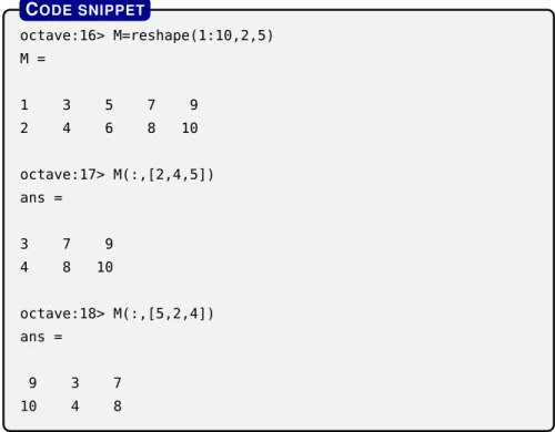
As for indexing in Octave, a somewhat uncommon indexing con- vention is employed as elements are indexed starting with1(as

(22)

octave:16> M=reshape(1:10,2,5) M =

1 3 5 7 9

2 4 6 8 10

octave:17> M(:,[2,4,5]) ans =

3 7 9

4 8 10

octave:18> M(:,[5,2,4]) ans =

9 3 7

10 4 8

CODE SNIPPET

Figure2.7: An illustration of indexing matrices in Octave.

opposed to0which is frequently encountered in most other programming languages). Figure2.7includes several examples of how indexing can be used to select certain elements from a matrix.

Figure2.7reveals a further useful property of Octave. Even if the result of a computation does not get assigned to a variable (or multiple variables) using the operator, the result of the lastly performed computation is automatically saved into an artificial variable, named ans(being a shorthand for answer). This variable acts as any other user created variable, so invoking something like2*ansis totally fine in Octave. Note however, that any upcoming command invoked in Octave will override the value stored in the artificial variableans, so in case we want to reutilize the results of a certain calculation, then we should definitely assign that result to a dedicated variable for future use.

2.1.5 Broadcasting

Recall the function from Figure2.5. At that point we argued that arguments must match their sizes in order arithmetic operations to make sense. That is, we can add and subtract two 5x6 matrices if we want, however, we are unable to perform such an operation between a 5x6 and a 5x7 matrices for instance.

What Octave does in such situations is that it automatically at- tempts to applybroadcasting. This means that Octave tries to make

(23)

%% generate 10000 100-dimensional observations X=rand(10000, 100);

tic

mu=mean(X);

X_centered=X;

for l=1:size(X,1)

X_centered(l,:) -= mu;

end toc

>>Elapsed time is 0.153826 seconds.

CODE SNIPPET

Figure2.8: Centering the dataset with forloop

the most sense out of operations that are otherwise incompatible from an algebraic point of view due to a mismatch in the sizes of their operands. Octave will certainly struggle with the previous example of trying to sum 5x6 and 5x7 matrices, however, there will be situations when it will provide us with a result even though our calculation cannot be performed from a linear algebraic point of view.

For instance, given some matrix A ^{n m}and a (column) vector b ^m ¹, the expressionA b is treated as if we were to calculate A 1b , with1denoting a vector in ⁿ ¹full of ones, i.e.

1 ... 1

. The outer product1b simply results in a matrix which contains the (row) vectorb in all of its rows and which has the same number of rows as matrixA.

tic

X_centered_broadcasted=X-mean(X);

toc

CODE SNIPPET

Figure2.9: Centering the dataset relying on broadcasting

Figure2.9illustrates broadcasting in action when we subtract the row vector that we get by calculating the column-wise mean values of matrixXand subtracting this row vector fromevery rowof matrixX in order to obtain a matrix which has zero expected value across all

of its columns. For an arbitrarily sized matrixA,

what would be the effect of the commandA-3? How would you write it down with standard linear algebra notation?

?

(24)

2.1.6 Vectorization

Vectorizationis the process when we try to express some sequential computation in the form of matrix operations. The reason to do so is that this way we can observe substantial speedup, especially if our computer enjoys access to some highly-optimized, hence extremely fast matrix libraries, such asBLAS(Basic Linear Algebra Subpro- grams),LAPACK(Linear Algebra PACKage),ATLAS(Automatically Tuned Linear Algebra Software) orIntel MKL(Math Kernel Library).

Luckily, Octave can build on top of such packages, which makes it really efficient when it comes to matrix calculations.

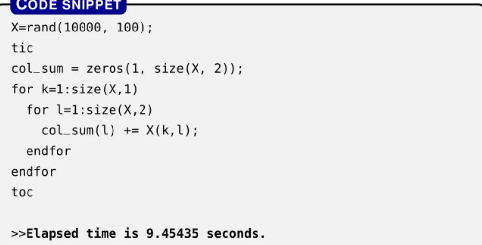
Suppose we are interested in the columnwise sums of some matrix X ^{m n}. That is, we would like to knows_l ^m_k ₁x_klfor every 1 l n. A straightforward implementation can be found in Fig- ure2.10, i.e., where we write two nested for loops to iterate over all thex_klelements of matrixXand for each index while incrementing the appropriate cumulative counters_l.

X=rand(10000, 100);

tic

col_sum = zeros(1, size(X, 2));

for k=1:size(X,1) for l=1:size(X,2)

col_sum(l) += X(k,l);

endfor endfor toc

CODE SNIPPET

Figure2.10: Calculating the columnwise sum of a matrix with aforloop.

We can, however, observe that matrix multiplications are also inherently applicable to express summations. This simply follows from the very definition of matrix multiplication, i.e., if we define Z XYfor any two matricesX ^{m n}andY ^{n p}, we have z_ij ⁿ_k ₁x_iky_kj. The code snippet in Figure2.11utilizes exactly this kind of idea upon speeding up substantially the calculation of the columnwise sums of our matrix by left multiplying it with a vector of all ones. By comparing the reported running times of the two implementations, we can see that the vectorized implementation has a more than5000-fold speedup compared to the one which explicitly uses for loops during the calculation even in the case of a moderately sized 10000 100 matrix.

(25)

tic

vectorized_col_sum = ones(1, size(X,1)) * X;

toc

CODE SNIPPET

Figure2.11: Calculating the columnwise sum of a matrix in a vectorized fashion withouta^forloop.

Note that we could have come up with a ’semi-vectorized’ implementation for calculating the columnwise sum of our matrix as illustrated in Figure2.12. In this case we are simply making use of the fact that summing up the row vectors in our matrix also provides us with the columnwise sums of our matrix. This way we can man- age to remove one of the unnecessary for loops, but we are still left with one of them. This in-between solution for eliminating needless loops from our implementation gives us a medium speedup, i.e., this versions runs nearly60-times slower than the fully vectorized one, however, it is still more than100-times faster compared to the non-vectorized version.

tic

semi_vectorized_col_sum=zeros(1,size(X,2));

for k=1:size(X,1)

semi_vectorized_col_sum += X(k,:);

end toc

CODE SNIPPET

Figure2.12: Calculating the columnwise sum of a matrix in a semi-vectorized fashion with single aforloop.

As another example, take the code snippets in Figure2.13and Figure2.14, both of which transforms a 10000 100 matrix such that after the transformation every row vector has a unit norm. Similar to the previous example, we have a straightforward implementation using a for loop (Figure2.13) and a vectorized one (Figure2.14). Just as before, running times are reasonably shorter in the case of the vectorized implementation.

The main take-away is that vectorized computation in general not only provides a more concise implementation, but one which is orders of magnitude faster compared to the non-vectorized solutions.

If we want to write efficient code (and most often – if not always – we do want), then it is crucial to identify those parts of our computation which can be expressed in a vectorized manner.

(26)

X=rand(10000, 100);

tic X_unit=X;

for l=1:size(X,1)

X_unit(l,:) /= norm(X(l,:));

end toc

CODE SNIPPET

Figure2.13: Transforming vectors in a matrix to unit-norm by relying on afor loop.

tic

norms=sqrt(sum(X.*X, 2));

X_unit_vectorized=X./norms;

toc

CODE SNIPPET

Figure2.14: Transforming vectors in a matrix to unit-norm in a vectorized fashionwithouta^forloop.

Writing a vectorized implementation might take a bit more effort and time compared to its non-vectorized counterpart if we are not used to it in the beginning, however, do not hesitate to spend the extra time cranking the math, as it will surely pay off in the running

time of our implementation. Can you think of a vectorized way

to calculate the covariance matrix of some sample matrixX? In case the concept of a covariance matrix sounds unfamiliar at the moment, it can be a good idea to look at Figure3.5.

2.2 Plotting ?

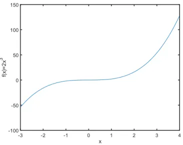
There is a wide variety of plotting functionalities in Octave. The simplest of all is the^plotfunction, which allows us to create simple x-y plots with linear axes. It takes two vectors of the same length as input and draws a curve based on the corresponding indices in the two vector arguments. Figure2.15illustrates the usage of the function with its output being included in Figure2.16.

x=-3:.01:4; % create a vector in [-3,4] with a step size 0.1 plot(x, 2*x.^3)

xlabel(’x’)

ylabel("f(x)=2x^3")

CODE SNIPPET

Figure2.15: Code for drawing a simple function f x 2x³over the range

3, 4 .

(27)

-3 -2 -1 0 1 2 3 4

-100 -50 0 50 100 150

f(x)=2x3

x

Figure2.16: The resulting output of the code snippet in Figure2.15for plotting the functionf x 2x³over the interval 3, 4 .

For the demonstration of further plotting utilities of Octave, con- sider the tiny example dataset found in Table2.1containing height and weight information of8people. Prior to running any core data mining algorithm on a dataset like that, it is often a good idea to fa- miliarize with the data first. Upon getting to know the data better, one typically checks out how the observations are distributed.

Possibly the simplest way to visualize the (joint) empirical distribution for a pair of random variables (or features in other words).

One can visualize the empirical distribution of the feature values by creating a so calledscatter plotbased on the observed feature values.

The Octave code and its respective output are included in Figure2.18 and Figure2.17, respectively.

By applying a scatter plot, one inherently limits himself/herself to focus on a pair of random variables, which is impractical for truly high-dimensional data that we typically deal with. Dimensionality reduction techniques, to be discussed in more detail later in Chap- ter6are possible techniques to aid the visualization of datasets with high number of dimensions.

height (cm) weight (kg)

187 92

172 77

200 101

184 92

162 70

176 81

172 68

166 55

Table2.1: Example dataset containing height and weight measurements of people.

scatter(D(:,1), D(:,2)) xlabel(’height (cm)’) ylabel(’weight (kg)’)

CODE SNIPPET

Figure2.17: Code for drawing a scatter plot of the heights of the people from the sample to be found in Table2.1.

The other frequently applied visualization form is for histograms, which aim to approximate some distribution by drawing an empirical frequency plot for the observed values. The way it works is that it divides the span of the random variable into a fixed number of

(28)

160 170 180 190 200 50

60 70 80 90 100 110

height (cm)

weight (kg)

Figure2.18: Scatter plot of the heights and weights of the people from the sample to be found in Table2.1.

equal bins and count the number of individual observations that fall within a particular range. This way, the more observations fall into a specific range, the higher bar is going to be displayed for that. A visual illustration of it and the corresponding Octave code which created it can be found in Figure2.19and Figure2.20, respectively.

hist(D(:,1),4)

xlabel(’height (cm)’) ylabel(’frequency’)

CODE SNIPPET

Figure2.19: Code for drawing a histogram of the heights of the people from the sample to be found in Ta- ble2.1.

160 170 180 190 200

0 0.5 1 1.5 2 2.5 3

frequency

height (cm)

Figure2.20: Histogram of the heights of the people from the sample to be found in Table2.1.

(29)

2.3 A brief comparison of Octave and numpy

In the recent years,Pythonhas gained a fair amount of popularity as well. Python is similar to Octave in that it is also a script language.

However, Python is intended to be a more general purpose programming language compared to Octave and it was not primarily designed for numerical computations. Thanks to the huge number of actively maintained libraries for Python, it is now also possible to perform matrix computations with the help of numpy and scipy packages (among many others).

It also has to offer similar functionalities to that of Octave in terms of data manipulation, including matrix calculations. In order to obtain the same core functionalities of Octave, which is of primarily interest for this book, one need to install and get to know a handful of non-standard Python packages, all with its own idiosyncrasy. For this reason, we will use Octave code throughout the book for illustra- tional purposes.

Sine there are relatively few major differences, someone fairly familiar with Octave can relatively quickly start writing Python code related to matrices. Perhaps the most significant and error-prone difference in the syntax of the two languages is that the operator denotes regular matrix multiplication in Octave (and its relatives such as Matlab), whereas the same operator when invoked for numpy multidimensional arrays, it acts as elementwise multiplication. The latter is often referenced as theHadamard productand denoted by .

X = [1 -2; 3 4];

Y = [-2 2; 0 1];

X*Y % perform matrix multiplication

>>ans =

-2 0

-6 10

X.*Y % perform elementwise multiplication

>>ans = -2 -4

0 4

CODE SNIPPET

Figure2.21: Comparing matrix-style and elementwise muliplication of matrices.

Recall that in Octave, whenever one wants to perform some elementwise operation, it can be expressed with an additional dot (.) symbol as already mentioned in Section2.1.4. For instance, . denotes elementwise multiplication in Octave. In order to see the differ-

(30)

ence between the two kinds of multiplication in action, see the code snippet in Figure2.21.

2.4 Summary of the chapter

Readers of this chapter are expected to develop familiarity with numerical computing, including the basic syntax of the language and also its idiosyncracies related to indexing, broadcasting and vectorization which allows us to write efficient code thanks to the highly optimized and parallelized implementation of the linear algebra packages Octave relies on in the background.

(31)

3 | B ASIC CONCEPTS

In t h i s c h a p t e rwe overview the main goal of data mining. By the end of the chapter, readers are expected to

• develop an understanding on the ways datasets can be represented,

• show a general sensitivity towards the ethical issues of data mining applications,

• be able to distinguish the different measurement scales of random variables and illustrate them,

• produce and efficiently implement summary statistics for the random variables included in datasets,

• understand the importance, apply and implement various data manipulation techniques.

Data miningis a branch of computer science which aims at pro- viding efficient algorithms that are capable of extracting useful knowledge from vast amounts of data. As an enormous amount of data gets accumulated by the everyday activities, such as watch- ing videos on YouTube, ordering products via Amazon, sending text messages on Twitter. As interacting with our environment gets tracked in an ever-increasing pace even for our most basic every day activities, there are a variety of ways in which data mining algorithms can influence our lives. Needless to say, there exists enormous application possibilities in applying the techniques of data mining with huge economic potential as well. As a consequence data has

often been coined as the new oil¹, due to the fact that having access ¹https://www.economist.com/leaders/2017/05/06/the- worlds-most-valuable-resource-is-no-

longer-oil-but-data

to data these days can generate such an economic potential to busi- nesses as fossil energy carrier used to do so. Handling the scale of data that is generated raises many interesting questions both in terms of scientific and engineering nature. In the following, we provide a few examples illustrating the incredible amount of data that is contin- uously being accumulated.

Learning Objectives:

• Goal of data mining

• Bonferroni principle

• Simpson’s paradox

• Data preprocessing steps

(32)

As an illustration regarding the abundance of data one can think of the social media platform Twitter. On an average day Twitter users compose approximately half a billion short text messages, meaning that nearly6,000tweets are posted every single second on average.

Obviously, tweets are not uniformly distributed over time, users being more active during certain parts of the day and particular events triggering enormous willingness to write a post. As an interesting trivia, the highest tweet-per-second (TPS) rate ever recorded up to

2018dates back to August2013, when143,199TPS was recorded². ²https://blog.twitter.

com/engineering/en_us/a/2013/

new-tweets-per-second-record-and-how.

html

Needless to say, analyzing this enormous stream of data can open up a bunch of interesting research questions one can investigate using

data mining and knowledge discovery³. ³Morstatter et al.2013,Gligoric et al.

As another example relating to textual data, Google revealed that 2018

its machine translation service is fed143billion words every single

day⁴as of2018. To put this amount of text into context – according to ⁴https://www.businessinsider.de/

sundar-pichai-google-translate-143-billion-words-daily-2018-7

Wikipedia⁵– this roughly corresponds to75,000copies of the world’s

5https://en.wikipedia.org/wiki/

List_of_longest_novels#List

longest novel which consists of10volumes and nearly2million words.

As an even more profound example, one can think of the experi- ments conducted at theLarge Hadron Collider(LHC) operated by CERN, the European Organization for Particle Physics. There are approximately1billion particle collisions registered in every second which yield an enormous amount of1Petabyte (10¹⁵bytes) of data.

As this amount of data would be unreasonable and wasteful to store directly, the CERN Data Centre distills it first so that1Petabyte of data to archive accumulates over a period of2–3days(instead of a single second) as the end of2017. As a consequence12.3Petabyte of data was archived to magnetic tapes during October2017alone and the total amount of permanently archived data surpassed200

Petabytes in the same year⁶. ⁶https://home.cern/

about/updates/2017/12/

breaking-data-records-bit-bit

3.1 Goal of data mining

Most real world observations can be naturally thought of as some (high-dimensional) vectors. One can imagine for instance each cus- tomer of a web shop as a vector in which each dimension of the vector is assigned to some product and the quantity along a particular dimension indicates the number of items that user has purchased so far from the corresponding product. In the example above, the possible outcome of a data mining algorithm could group customers with similar product preferences together.

The general goal of data mining is to come up with previously unknown valid and relevant knowledge from large amounts of data sets. For this reason data mining and knowledge discovery is some-

(33)

b a s i c c o n c e p t s 33

times referred as synonyms, the schematic overview of which is summarized in Figure3.1.

Figure3.1: The process of knowledge discovery

3.1.1 Correlation does not mean causality

A common fallacy when dealing with datasets is to use correlation and causality interchangeably. When a certain phenomenon is caused by another, it is natural to see high correlation between the random variables describing the phenomena being in a causal relationship.

This statement is not necessarily true in the other direction, i.e., just because it is possible to notice a high correlation between two random variables it need not follow that any of the events have a causal effect on the other one.

Kentucky marriages

Fishing boat deaths

People who drowned after falling out of a fishing boat correlates with

Marriage rate in Kentucky

Kentucky marriages Fishing boat deaths

1999 2000 2001 2002 2003 2004 2005 2006 2007 2008 2009 2010

7 per 1,000 8 per 1,000 9 per 1,000 10 per 1,000 11 per 1,000

0 deaths 10 deaths 20 deaths

tylervigen.com

Figure3.2: Example of a spurious correlation. Source:

http://www.tylervigen.com/

spurious-correlations

Figure3.2shows such a case when high correlation between two random variables (i.e., the number of people drowned and the marriage rate in Kentucky) is very unlikely to be in causal relationship with each other.

(34)

3.1.2 Simpson’s paradox

Simpson’s paradox also reminds us that we shall be cautious when drawing conclusions from some dataset. As an illustration for the paradox, inspect the hypothetical admittance rates of an imaginary university as included in Table3.1. The admittance statistics are broken down with respect the gender of applicants and the major that they applied for.

Applied/Admitted Female Male Major A 7/100 3/50 Major B 91/100 172/200 Total 98/200 175/250

Table3.1: Example dataset illustrating Simpson’s paradox

At first glance, it seems that females have a harder time getting admitted to the university overall, as their success rate is only49% (98admitted out of200), whereas males seem to get admitted more seamlessly with a70% admittance rate (175out of200). Looking at these marginalized admittance rates, decision makers of this university might suspect that there might be some unfair advantage given to male applicants.

Looking at the admittance rates broken down to each major on the other hand, shows us a seemingly contradictory pattern. For Major A and B female applicants show a7% and91% success rate, respectively, compared to the6% and86% success rate for males. So, somewhat counter-intuitively, females have a higher acceptance rate than males on both major A and B, yet their aggregated success rate falls behind that of males. Before reading onwards, can you come up with an explanation for this mystery?

In order to understand what is causing this phenomenon, we have to observe that females and males have a different tendency towards applying for the different majors. Females tend to apply in an even fashion as there are100–100applicants for both Major A and B, however, for the males there is a preference towards Major B, which seems to be an easier way to go for in general. Irrespective of the gender of the applicant, someone who applied to Major B was admitted with87.7% chance, i.e., (91+172)/(100+200), whereas the gender-agnostic success rate is only6.7% for Major A, i.e., only10 people out of the150applicants were admitted for that major.

Thelaw of total probabilitytells us how to come up with probabilities that are ’agnostic’ towards some random variable. In a more rigorous mathematical language, defining some observation-agnostic probability is called marginalization and the probability we obtain as

(35)

b a s i c c o n c e p t s 35

marginal probability.

Let us define random variableMas a person’s choice for a major to enroll to andGas the gender a person. Formally, given these two random variables, the probability for observing a particular realiza- tionmfor variableMcan be expressed as a sum of joint probabilities over all the possible valuesgthat random variableGcan take on.

Formally,P M m

g G

P M m,G g .

Another concept we need to be familiar with is theconditional probabilityof some eventM mgivenG g. This is defined asP M m G g ^{P M m,G g}_{P G g} , i.e., the fraction of the joint probability of the two events divided by the marginal probability of the event on which we wish to condition on. If we introduce another random variableSwhich indicates if an application is successful or not, we can express the following equalities by relying on the definition of the conditional probability

P S s M m,G g P M m G g

P S s,M m,G g

P M m,G g

P G g

P G g,M m,G g

P G g

P S s,M m G g .

This means that the probability of a person being successfully admitted to a particular majorgivenhis/her gender can be decomposed into the product of two conditional probabilities, i.e.,

1. the probability of being successfully admittedgiventhe major he/she applied for and his/her gender and

2. the probability of applying for a particular majorgivenhis/her gender.

Recalling the law of total probability, we can define probability that someone is successfully admittedgivenhis/her gender as

P S s G g

m A,B

P S s,M m G g

m A,B

P S s M m,G g P M m G g .

Based on that, the admittance probability that for females emerges as

P S success G f emale 100 200

7 100

100 200

91 100

98

200 0.49, whereas that for males is

P S success G male 3

50 50 250

172 200

200 250

175 250 0.7.

(36)

This break-down for the probability of the success for the different genders unveils that the probability that we observe in the major- agnostic case can deviate from the probability for success that we get for the major-aware case. The reason for the discrepancy was due to the fact that females had an increased tendency for applying to the major which was more difficult to get in. Once we look at the admittance rates for the two majors separately, we can see, that it were actually the female applicants which were more successful during their applications.

3.1.3 Bonferroni’s principle

Bonferroni’s principlereminds us that if we repeat some experiment multiple times, we can easily observe some phenomenon to occur frequently purely originating from our vast amount of data that we are analyzing. As a consequence, it is of great importance that whenever we notice some seemingly interesting pattern of high frequency, to be aware of the number of times we were about to observe that given pattern purely due to chance. This way we can mitigate the effects of creating false positive alarms, i.e., claiming that we managed to find something interesting when this is not the case in reality.

Let us suppose that all the people working at some imaginary factory are asocial at their workspace, meaning that they are absolutely uninterested in becoming friends with their co-workers. The manager (probably unaware of the employees not willing to make friendships) decides to collect pairs of workers who could become soul mates.

The manager defines potential soul mates as those pair of people who order the exact same dishes during lunchtime at the factory canteen where the workers can choose betweenssoups,mmain dishes anddmany desserts. For simplicity let us assume that the canteen servess m d 6 kind of meals each forw 1, 200 workers and the experiment runs over one week. The question is, how many potential soul mates would we find under these conditions by chance?

Let us assume that the employees do not have any dietary restric- tions and have no preference among the dishes the canteen can offer, for which reason they select their lunch every day randomly. This means that there ares m d 6³ 216 many equally likely different combinations of lunches for which reason, the probability of a worker choosing a particular lunch configuration (a soup, main course, dessert triplet) is 6 ³ 0.0046.

It turns out that the probability of two workers choosing the same lunch configurations independently have the exact same probability as one worker going for a particular lunch. Since every employee has 216 options for the lunch, the number of different ways a pair