Approximation of the Whole Pareto Optimal Set for the Vector Optimization Problem
In Memoriam András Prékopa (1929-2016)
Tibor Illés
1, Gábor Lovics
21Optimization Research Group, Department of Differential Equations, Budapest University of Technology and Economics, Egry József u. 1., 1111 Budapest, Hungary,
illes@math.bme.hu
2Hungarian Central Statistical Office, Keleti Károly u. 5-7., 1024 Budapest, Hungary, Gabor.Lovics@ksh.hu
In multi-objective optimization problems several objective functions have to be minimized simultaneously. In this work, we present a new computational method for the linearly con- strained, convex multi-objective optimization problem. We propose some techniques to find joint decreasing directions for both the unconstrained and the linearly constrained case as well. Based on these results, we introduce a method using a subdivision technique to ap- proximate the whole Pareto optimal set of the linearly constrained, convex multi-objective optimization problem. Finally, we illustrate our algorithm by solving the Markowitz model on real data.
Keywords: multi-objective optimization; joint decreasing direction; approximation of Pareto optimal set; Markowitz model
2000 MSC: 90C29
1 Introduction
In the literature of economics and finance the measure of risk has always been a very interesting topic, and nowadays it may be even more important than ever. One of the first idea to be taken into consideration is the risk in financial activities coming from Markowitz [26], who developed his famous model, where the investors make portfolios from different securities, and try to maximize their profit and minimize their risk at the same time. In this model, the profit was linear and the risk was defined as the variance of the securities. The Markowitz model can be formulated as a linearly constrained optimization problem with two objective (linear profit and quadratic risk) functions.
In the general case, the least risky portfolio is not the most profitable one; thus we could not optimize the two objectives at the same time. Therefore, we need to find portfolios, where one of the goals cannot be improved without worsening the
other. This kind of solutions are calledPareto optimalorPareto efficientsolutions discussed by Pareto [30].
Single Pareto optimal solution of the Markowitz model can be computed by scalar- ization methods, see Luc [23] and Miettinen [28], where the weighted sum of the objective functions, serving as a new objective function, defines a single quadratic objective function. Therefore, after the scalarization of the Markowitz model, the optimization problem simplifies to a quadratic optimization problem over linear constraints [25]. The simplified problem’s optimal solution is a single Pareto op- timal solution of the original problem. The effect of the weights of the objective functions determine the computed Pareto efficient solution of the original problem.
The weights might have unpredictable effects on the computed Pareto efficient so- lution in general. Weakness of this approach is that it restricts the Pareto efficient solution set to a single element and it’s local neighborhood. In this way, we lose some information, like how much extra profit can be gained by accepting a larger risk. Finding - or at least approximating - the whole Pareto efficient solution set of the original, multi-objective problem, may lead to a better understanding of the modeled practical problem [27].
For some unconstrained multi-objective optimization problems there are research papers [7, 8, 13, 34] discussing algorithms applicable for approximating the Pareto efficient solution set. However, many multi-objective optimization problems - natu- rally - have constraints [13, 14]. A simple example for a constrained multi-objective optimization problem is the earlier mentioned Markowitz model. In this paper, we extend and generalize the algorithm of Dellnitz et al. [7] for approximating the Pareto efficient set of a linearly constrained convex multi-objective problem. Fliege and Svaiter [13] obtained some theoretical results, that are similar to our approach for finding joint decreasing directions.
In the next section, most important definitions and results of vector optimization problems are summarized. In the third section, we discuss some results about the unconstrained vector optimization problem. The method called subdivision tech- nique introduced by Dellnitz et al. [7, 8] was developed to approximate the Pareto efficient solution set of an unconstrained vector optimization problems. The subdi- vision method uses some results described in [34]. An important ingredient of all methods, that can approximate the Pareto optimal set of a convex vector optimiza- tion problem, is the computation of a joint decreasing direction for all objective functions. We show that - using results from linear optimization - a joint decreasing direction for an unconstrained vector optimization problem can be computed.
In the fourth section, the computation of a feasible joint decreasing direction for linearly constrained convex vector optimization problem is discussed. The set of feasible joint decreasing directions forms a finitely generated cone and can be com- puted, as shown in Section 4. Interesting optimality conditions of Eichfelder and Ha [10] for multi-objective optimization problems show some similarities to those that are used in this paper during the computations of joint decreasing directions;
however their results do not have practical, algorithmic applications yet.
Section 5 contains an algorithm, which is a generalization of the subdivision method
for the linearly constrained convex vector optimization problem. In Section 6, we show some numerical results obtained on a real data set (securities from Budapest Stock Exchange) for the Markowitz model.
Comparing our method presented in Section 5, with the subdivision algorithm of Dellnitz et al. [7, 8], clearly, our method works for unconstrained vector optimiza- tion problems (UVOP), like that of Dellnitz et al. [7, 8], but we generate different joint decreasing directions. Furthermore, our method is applicable to vector op- timization problems (VOP) with convex objective functions and linear constraints, keeping all advantageous properties of subdivision algorithm of Dellnitz et al. [7,8].
For the (VOP) there are some sophisticated scalarization methods reported in [15].
This method, as scalarization methods in general, finds a single Pareto optimal solu- tion. The scalarization method introduced by [15] defines a weighted optimization problem (WOP) of (VOP) with fixed weights and a feasible solution set, that de- pends on the current feasible vectorx. Thus, in each iteration of the algorithm the actual feasible solution set is restricted to such a subset of the original feasible so- lution set, where some Pareto optimal solutions are located.
Subdivision techniques - including ours - find a cover set of the Pareto optimal solution set, formed by boxes used in the subdivision procedure (see Sections 5 and 6). The approximation of the whole Pareto optimal solution set is controlled by the diameter of the covering boxes computed in the subdivision procedure of the algorithm.
Although both the scalarization algorithm of Gianessi et al. [15] and our subdivision algorithm have some similarities (i.e., in each iteration the feasible solution set de- creases), there are significant differences as well. The scalarization algorithm finds a single Pareto optimal solution under some quite general assumptions, while the subdivision algorithm approximates the whole Pareto optimal solution set for the (VOP) with convex objective functions and linear constraints.
We use the following notations throughout the paper: scalars and indices are denoted by lowercase Latin letters, column vectors by lowercase boldface Latin letters, ma- trices by capital Latin letters, and finally sets by capital calligraphic letters.
The vector, with all 1 elements is denoted bye, i.e.
eT := (1,1, . . . ,1)∈Rn,
for somen∈N, whereT stands for the transpose of a (column) vector (or a matrix).
Vectorei∈Rnis theith unit vector of thendimensional Euclidean space.
2 Basic Definitions and Results in Vector Optimization
In this section, we discuss some notations, define the vector (or multi-objective) optimization problem and the concept of Pareto optimal solutions. Furthermore, we state two well known results of vector optimization, which are important for our approach.
We define theunit simplex set, as,
Definition 1. LetSk denote the unit simplex in the k dimensional vector space, and define it as follows:
Sk:={w∈Rk: eTw=1, w≥0}.
LetF ⊆Rnbe a set andF:F→Rkis a function defined as F(x) = [f1(x),f2(x), . . . ,fk(x)]T,
where fi:F →Ris a coordinate function for alli.
Thegeneral vector optimization problem(GV OP)can be formulated as
(GV OP) MINF(x), subject to x∈F.
If the setF and the functionF are convex, then(GV OP)is aconvex vector opti- mization problem. We assume thatFis differentiable.
Usually, different objective functions of(GV OP)describe conflicting goals, there- fore suchx∈F, that minimize all objective functions at the same time, is unlikely to exist. For this reason, the following definitions naturally extend the concept of an optimal solution for(GV OP)settings.
Definition 2. Let(GV OP)be given. We say thatx∗∈F is a
1. weakly Pareto optimal solutionof problem(GV OP)if there does not exist a feasible solutionx∈F which satisfies the vector inequality F(x)<F(x∗);
2. Pareto optimal solutionif does not exist feasible solutionx∈F which satis- fies the vector inequality F(x)≤F(x∗)and F(x)6=F(x∗).
Furthermore, we call the setF∗⊆F aweakly Pareto optimal setif every x∗∈F∗ is a weakly Pareto optimal solution of the(GV OP).
Our goal is to approximate the whole Pareto optimal or weakly Pareto optimal so- lution sets for different vector optimization problems. During the approximation procedure of the whole Pareto optimal solution set, we compute many Pareto op- timal solutions and produce an outer approximation of the whole Pareto optimal solution set.
The literature contains several methods that, find one of the Pareto optimal solutions, see [9, 23, 28], but sometimes it is interesting to compute all of them, or at least as much as we can.
One of the frequently used method to compute a Pareto optimal solution uses a weighted sum of the objective functions to obtain a single objective optimization problem. Letw∈Sk be a given vector of weights. From a vector optimization problem, using a vector of weights, we can define the weighted optimization prob- lem as follows
(W OP) minwTF(x), subject to x∈F.
We state without proof two well-known theorems, that describe the relationship between(GV OP)and(W OP). The first theorem shows that the(W OP)can be used to find a Pareto optimal solution, see for instance [9, 23, 28].
Theorem 1. Let a(GV OP)and the corresponding(W OP)for aw∈Skbe given.
Assume thatx∗∈F is an optimal solution of the(W OP)problem; thenx∗is a weak Pareto optimal solution for the(GV OP).
Next theorem needs a bit more complicated reasoning, but for the convex case each Pareto optimal solution of the (GV OP)can be found through a(W OP)using the proper weights [9, 23, 28].
Theorem 2. Let(GV OP)be a convex vector optimization problem, and assume that x∗∈F is a Pareto optimal solution of the(GV OP); then there is aw∈Skweight vector, and a(W OP)problem, for whichx∗is an optimal solution.
The method, that will be described in section 5, decreases every coordinate function ofFat the same time and always moves from a feasible solution to another feasible solution; hence we introduce the following useful definition.
Definition 3. Let problem (GV OP)and feasible pointx∈F be given. Vector v∈Rn,v6=0is called a
1. joint decreasing directionat pointxiff there exists h0>0for every h∈]0,h0] satisfying that
F(x+hv)<F(x);
2. feasible joint decreasing direction iff it is a joint decreasing direction and there exists h1>0such that, for every h∈]0,h1]we havex+hv∈F. Example. Let the following unconstrained vector optimization problem (GV OP1) MINF(x1,x2) =
f1(x1,x2) =x21+x22
f2(x1,x2) = (x1−1)2+ (x2−1)2
,
be given alongside a pointxT = (x1,x2) = (0,1)and directionvT = (1,−1). Now we show thatvis a joint decreasing direction for the objective functionFat pointx.
It is easy to show that
f1(x+hv) =f2(x+hv) =h2+ (1−h)2=2
h−1 2
2
+1 2
From the last form of the coordinate functions, it is easy to see that the coordi- nate functions are decreasing on the[0;12]interval; thereforevis a joint decreasing direction withh0=12.
If we add a single constraint to our example, then we obtain a new problem
(GV OP2) MINF(x1,x2) =
f1(x1,x2) =x21+x22
f2(x1,x2) = (x1−1)2+ (x2−1)2
, subject to x1≤1
3.
It is easy to see thatvis a feasible joint decreasing direction for problem(GV OP2) too, withh1=13.
From now on, let us consider(GV OP)with a convex, differentiable objective func- tionFand let us denote the Jacobian-matrix ofF at pointxbyJ(x). Then,v∈Rn is a joint decreasing direction of functionFat pointx, if and only if
[J(x)]v<0, (1)
asvis a decreasing direction for theith coordinate function fiat pointx, if and only if[∇fi(x)]Tv<0.
3 Results for Unconstrained Vector Optimization
In this section, we review some results of unconstrained vector optimization, namely for F =Rn. We assume thatF is a differentiable function. The unconstrained vector optimization problem is denoted by(UV OP).
Before we show how a joint decreasing direction can be computed, we need a cri- terion to decide wether anxis a Pareto optimal solution or not, see Schäffler et al.
[34].
Definition 4. Let J(x)∈Rk×nbe the Jacobian matrix of a differentiable function F :Rn→Rkat a pointx∈Rn. Anx∗is calledsubstationary pointof F iff there exist aw∈Sk, which fulfills the following equation:
wT[J(x∗)] =0.
In the unconstrained case, pointx∗is a substationary point of the objective function Fof (GVOP), if it is a stationery point of the weighted objective function of(W OP).
From Theorem 1 and Theorem 2 we can see that in convex case, substationary points are weak Pareto optimal solutions of the unconstrained vector optimization problem (GVOP).
We are ready to discuss two models to find joint decreasing directions. The first model has been discussed in [34] and uses a quadratic programming problem formu- lation to compute joint decreasing directions. Later we show that a joint decreasing direction can be computed in a simpler way by using a special linear programming problem.
Let us define the following quadratic programming problem(QOP(x))for anyx∈ Rn, with variablew
(QOP(x)) minwT
J(x) [J(x)]T
w, subject to w∈Sk.
From the well known Weierstarss Theorem it follows that this problem always has an optimal solution, since the feasible set is compact and the function
g:Sk→R, g(w) =wT
J(x) [J(x)]T w
is a convex, quadratic, continuous function for any givenx∈Rn.
Next theorem is an already known statement [34, Theorem 2.1], for which we give a new and shorter proof. This shows that using the(QOP(x))problem we can find a joint decreasing direction ofFor a certificate thatxis a Pareto optimal solution of problem(UV OP).
Theorem 3. Let a problem(UV OP), a pointx∈Rnand the associated(QOP(x)) be given. Letw∗∈Rkdenote the optimal solution of(QOP(x)). We define vector q∈Rnasq= [J(x)]Tw∗. Ifq=0, thenxis a substationary point, otherwise−qis a joint decreasing direction for F at pointx.
Proof. Whenq=0then Definition 4 shows thatx is substationary point. When q6=0, we indirectly assume that−qis not a decreasing direction for theith coor- dinate function, fi ofF and[∇fi(x)]Tq6=0. It means that[∇fi(x)]Tq<0. Since [∇fi(x)]T =eTi J(x), so our indirect assumption means
[∇fi(x)]Tq=eTi[J(x)][J(x)]Tw∗<0.
We show thatei−w∗6=0is a feasible decreasing direction ofg(w∗)which contra- dicts the optimality ofw∗. Theei=w∗can not be fulfilled because it contradicts the indirect assumption, and it is easy to see, thateiis a feasible solution of(QOP(x)) soei−w∗is a feasible direction at pointw∗.
Since
∇g(w) =2[J(x)][J(x)]Tw thus
[∇g(w∗)]T(ei−w∗) =2w∗T[J(x)][J(x)]T(ei−w∗)
=2w∗T[J(x)][J(x)]Tei−2w∗T[J(x)][J(x)]Tw∗
=2qT[∇fi(x)]−2w∗T[J(x)][J(x)]Tw∗<0,
where the first term of the sum is negative because of the indirect assumption, and the second term is not positive, because[J(x)][J(x)]T is a positive semidefinite ma- trix.
The previous result underline the importance of solving (QOP(x))problem effi- ciently. For solving smaller size linearly constrained convex quadratic problems
pivot algorithms [1, 4–6, 16, 22] can be used. In case of larger size linearly con- strained, convex quadratic problems, interior point algorithms can be used to solve the problem (see for instance [18, 20]).
Theorem 3 shows that a joint decreasing direction can be computed as the convex combination of the gradient vectors of coordinate functions of F. Following the ideas discussed above, we can formulate a linear programming problem such that any optimal solution of the linear program defines a joint decreasing direction of problem(UV OP). Some similar results can be found in [13].
Let us define the linear optimization problem(LP(x))in the following way:
(LP(x)) maxq0, subject to [J(x)]q+q0e≤0, 0≤q0≤1,
whereq∈Rnandq0∈Rare the decision variables of the problemLP(x). Now we are ready to state and prove a theorem that discusses a connection between(UV OP) and(LP(x)).
Theorem 4. Let a pointx∈Rn, an(UV OP)and an associated(LP(x))be given.
Then the(LP(x))always has an optimal solution(q∗,q∗0). There are two cases for the optimal value of the(LP(x)), either q0=0thusxis a substationary point of the (UV OP), or q0=1thusq∗is a joint decreasing direction for the function F at point x.
Proof. It is easy to see thatq=0,q0=0 is a feasible solution of problem(LP(x)) and 1 is an upper bound of the objective function, which means(LP(x))should have an optimal solution.
Let us examine the case
[J(x)]q+q0e≤0, q0>0. (2)
If system (2) has a solution, than 1
q0q,1
is a solution of the system, so the optimal value of the objective function is 1. This mean that
[J(x)]q≤ −e
so theqis a joint decreasing direction of functionF.
If the system (2) has no solution then the optimal value of the objective function is 0, and from the Farkas lemma ([11, 12, 17, 22, 29, 31, 32, 35]) we know that there exists awwhich satisfies the following:
wT[J(x)] =0, eTw=1, w≥0. (3)
It means that if the optimal value of the problem(LP(x))is 0, thanxis a substation- ary point.
A linear programming problem(LP(x))(and later on(LPS(x))) can be solved by either pivot or interior point algorithms, see [21]. In case of applying pivot methods to solve linear programming problem, simplex algorithm is a natural choice, see [24,
29, 35]. A recent study on anti-cycling pivot rules for linear programming problem contains a numerical study on different pivot algorithms, see [6]. Sometimes, if the problem is well structured and small, criss-cross algorithm of T. Terlaky can be used for solving the linear programming problem as well, see [17, 36]. More about interior point algorithms for linear programming problems can be learnt from [19, 24, 33].
In this section two techniques were introduced to decide whether a pointxis a weak Pareto optimal solution of problem(UV OP)or to find a joint decreasing direction.
Before we generalize this result to the linear constrained case let us compare this technique with some known procedures. The classical scalarization technique based on(W OP)finds a Pareto optimal solutionx∗of(UV OP). Due to the requirements defined by the concept of the weak Pareto optimal solution, it may happen that in some iterations of the scalarization algorithm such feasible solutions are computed for which some objective function’s value increases. In our method this phenomena can not happen, because in each iteration we select a joint decreasing direction.
4 Vector Optimization with Linear Constraints
In this section, we show how we can find a feasible joint decreasing direction for linearly constrained vector optimization problems. First we find a feasible joint decreasing direction for a special problem, where we only have sign constraints on the variables. After that we generalize our results to general linearly constrained vector optimization problems. Our method can be considered as the generalization of the well known reduced gradient method to vector optimization problems. Some similar result can be found in [13], for the feasible direction method of Zountendijk.
First we define the vector optimization problem with sign constraints(SV OP):
(SV OP) MIN F(x), subject to x≥0,
whereF is a convex function. From Theorem 1 we know thatx∗≥0 is a Pareto optimal solution if there exists aw∈Skvector such thatx∗is an optimal solution of
(SW OP) minwTF(x), subject to x≥0.
Since Slater regularity and convexity conditions hold, from the KKT theorem [24]
we know thatx∗≥0is an optimal solution of(SW OP)iff it satisfies the following system:
wT[J(x∗)]≥0, wT[J(x∗)]x∗=0. (4) Let the vector x≥0be given and we would like to decide wether it is an optimal solution of the (SWOP) problem or not. Let us define the index sets
I+={i:xi>0}, and I0={i:xi=0},
that depend on the selected vectorx. Using the index setsI0,I+, we partition the column vectors of matrixJ(x)into two parts. The two parts are denoted byJ(x)I0 and J(x)I+. Taking into consideration the partition, the KKT conditions can be written in an equivalent form as
wT[J(x)]I+=0, wT[J(x)]I0≥0, w∈Sk. (5) The inequality system (5) plays the same role for (SV OP) as (3) for (UV OP), namelyxis a Pareto-optimal solution if (5) has a solution.
Now we can define a linear programming problem corresponding to(SV OP)such that an optimal solution of the linear programming problem either defines a joint decreasing direction or gives a certificate that the solution x is a Pareto optimal solution of(SV OP).
(LPS(x)) maxz,
subject to [J(x)]I+u+ [J(x)]I0v+ze≤0, v≥0, 0≤z≤1,
whereu,vandzare the decision variables of problem (LPS(x)). Now we are ready to prove the following theorem.
Theorem 5. Let a(SV OP)and an associated(LPS(x))be given, wherex∈F is a feasible point. The problem(LPS(x))always has an optimal solution(u∗,v∗,z∗).
There are two cases for the optimal value of problem(LPS(x)), z∗=0which means that x is a Pareto optimal solution of the (SV OP), or z∗=1 which means that qT= (u∗,v∗)is a feasible joint decreasing direction of function F.
Proof. It is easy to see thatu=0,v=0,z=0 is a feasible solution of the problem (LPS(x))and 1 is an upper bound of the objective function, therefore(LPS(x))has an optimal solution.
Let us examine the following system
[J(x)]I+u+ [J(x)]I0v+ze≤0, v≥0, z>0. (6) If system (6) has a solution, then 1zu,1zv,1
is an optimal solution of the problem (LPS(x))with optimal value 1. Thus the vectorqT = (u,v)satisfies
[J(x)]q≤ −e<0,
so theqis a feasible joint decreasing direction for functionF atx∈F. Vectorqis feasible becauseqI0 =v≥0.
If the system (6) has no solution then the optimal value of the objective function is 0, and from a variant of the Farkas lemma, see [11, 12, 17, 22, 31, 32, 35] we know that there exists awwhich satisfies the following system of inequalities:
[J(x)]TI
+w=0, [J(x)]TI
0w≥0, eTw=1, w≥0. (7)
It means that if the optimal value of problem(LPS(x))is 0, then pointxis a Pareto optimal solution of (SVOP).
We are ready to find feasible joint decreasing direction to a linearly constrained vector optimization problem at a feasible solution ˜x. Let the matrixA∈Rm×nand vectorb∈Rmbe given. Without loss of generality we may assume thatrank(A) = m. Furthermore, let us assume the following non degeneracy assumption (for details see [2]): anymcolumns ofAare linearly independent and every basic solution is non degenerate. We have a vector optimization problem with linear constraint in the following form
(LV OP) MINF(x), subject to Ax=b, x≥0.
Like in the reduced gradient method, see [2], we can partition the matrixAinto two partsA= [B,N], whereBis a basic andNthe non-basic part of the matrix. Similarly everyv∈Rnvector can be partitioned asv= [vB,vN]. We callvBbasic andvN a nonbasic vector. We can chose the matrixBsuch that the ˜xB>0 is fulfilled. While Ax=bholds, we know that
BxB+NxN=b, and xB=B−1(b−NxN).
We can redefine functionFin a reduced form as FN(xN) =F(xB,xN) =F(B−1(b−NxN),xN).
Let us define using the partition(B,N)and the following sign constraint optimiza- tion problem
(SV OPB(˜x)) MINFN(xN), subject to xN≥0.
Let qN denote a feasible joint decreasing direction for (SV OPB(˜x)) at point ˜xN, which can be found by applying Theorem 5. Let qB=−B−1NqN; then we show thatq= [qB,qN]is feasible joint decreasing direction for(LV OP)at point ˜x. Let us notice that
A(˜x+hq) =Ax˜+h(BqB+NqN) =b+h −B(B−1NqN) +NqN
=b,
for every h∈R. So FN(˜x+hqN) =F(˜x+hq) and whileqN is a feasible joint decreasing direction withh1>0 stepsize for(SV OPB(˜x)). We can show thatqis a joint decreasing direction for problem (LV OP)with the sameh1>0 step size.
While ˜xB>0, there existsh2>0, such that ˜xB+h2qB≥0, thereforeqis a feasible joint decreasing direction for problem(LV OP)with a step-size
h3=min(h1,h2)>0. (8)
We can computeh1andh2using a ratio-test, since ˜xi+hqi≥0 for alliis required, therefore
h1=min
−x˜i
qi : qi<0, i∈N
>0,and h2=min
−x˜i
qi : qi<0, i∈B
>0.
5 The Subdivision Algorithm for Linearly Constrained Vector Optimization Problem
In this section, we show how can we build a subdivision method to approximate the Pareto optimal set of a linearly constrained vector optimization problem. Our method is a generalization of the algorithm discussed in [7], where you can find some results about convergence of the subdivision technique. The original method can not handle linear constraints.
Our algorithm approximates the Pareto optimal solution setF∗, using small boxes that each contains at least one computed Pareto optimal solution. The smaller the sets, the better approximation of theF∗, therefore we define the following measure of sets involved in the approximation ofF∗.
Definition 5. LetH ⊆Rnbe given; thediameterofH is defined as diam(H):= sup
x,y∈H||x−y||.
LetHbe a family of sets, which contains a finite number of sets fromRn; then the diameterofHis
diam(H) =max
H∈H
diam(H).
Let us assume that the feasible set of our problem is nonempty, closed and bounded.
In this case Pareto optimal solution set of the problem(LV OP)is a nonempty set, defined as,
FL∗={x∈F :xis Pareto optimal solution of(LV OP)}.
Based on our assumption, thatF is bounded set, there exists H0={x∈Rn|l≤x≤u},
wherel,u∈Rnare given vectors and FL∗⊆F ⊆H0∩ {x∈Rn:Ax=b}.
Our goal is to introduce such a subdivision algorithm for(LV OP)problem, that iter- atively defines better and better inner and outer approximation of the Pareto optimal solution set of a problem(LV OP). The inner approximation will be an increasing sequence of setsF Pi, containing finitely many Pareto optimal solutions produced by the algorithm. The outer approximation will be a family of setsHiproduced in each iteration of the algorithm, that coversFL∗with decreasing diameter,diam(Hi).
The input of our method are data of the (LVOP) problem, namely matrixA∈Rm×n, vectorb∈Rm, functionF:Rn→Rk, setH0and a constantε>0.
The output of our algorithm is a family of setsH, such thatdiam(H)<εand each H ∈Hcontains at least one Pareto optimal solution.
The algorithm uses some variables and subroutines, too. TheS P,F Pare finite- element sets of points fromRn,H,G ⊆F,H0,K,K0andAare family of sets like H.
Our algorithm in the first step defines the family of setsH, which contains only the H0set. The cycle in step 2 runs while the diameter ofHis not small enough. The algorithm reaches this goal in a finite number of iteration, because as you will see in subroutine Newset(H) the diameter ofHconverges to zero. Nevertheless we show that after every execution of the cycle the family of setsHcontains setsH which have Pareto optimal solutions. At the beginning it is trivial, becauseHcontain the whole feasible set.
Subdivision algorithm for (LVOP)
1. H={H0}
2. Whilediam(H)≥εdo (a) H0=Newsets(H) (b) S P=/0 (c) WhileH6=/0do
i. H ∈H
ii. S P=S P∪Startpoint(H) iii. H=H\ {H}
End While
(d) F P=Points(S P,A,b,F) (e) WhileH06=/0do
i. H ∈H0
ii. IfH ∩F P6=/0thenH=H∪ {H}End If iii. H0=H0\ {H}
End While End While 3. Output(H)
In step 2(a) we define a family of setsH0using the subroutine Newset(H). The sets fromH0 are smaller than sets formHand cover the same set. Therefore the result of this subroutine has two important properties:
1. ∪H∈H0(H ∩F) =∪H∈H(H ∩F), 2. diam(H0) =K1diam(H),
whereK>1 is a constant.
The steps in cycle 2, from step 2(b), delete the sets fromH0 which do not contain any Pareto optimal points. Step 2(b) makes setS Pempty. The cycle in step 2(c) produces a finite number of random starting points in setH ∩ {x∈Rn:Ax=b}for everyH ∈Husing subroutine Startpoint(H), and puts the generated points into the setSP.
The main step of our algorithm 2(d) is the subroutine Points(S P,A,b,F) that pro- duce a set F P which contains Pareto optimal points. This subroutine uses our results from Section 4.
In cycle 2(e) we keep every set from H0which contains Pareto optimal solutions and add those toH. Finally, we check the length of the diameter ofHand repeat the cycle until the diameter is larger than the accuracy parameterε.
SubroutinePoints(S P,A,b,F) 1. WhileS P6=/0do
(a) s∈S P (b) x=s,z=1 (c) Whilez=1do
i. (B,N) =A ii. (xB,xN) =x
iii. (q,z)=Solve(LPS(xN)) iv. Ifz=1then
A. h3=stepsize(F,B,N,b,xN,q) B. xN =xN+h3q
C. xB=b−B−1NxN D. x= (xB,xN) End If
End While (d) S P=S P\ {s}
(e) F P=F P∪ {x}
End While 2. Output(F P)
Subroutine Points uses a version of the reduced gradient method for computing Pareto optimal solutions or joint decreasing directions, as discussed in Section 4.
This subroutine works until from all points inS Psearch for a Pareto optimal point has been executed. The cycle 1(c) runs until it finds a Pareto optimal point. As we discussed in section 4 the cycle finishes whenz=0. In line 1(c)i the matrixAis partitioned into a basic and a non basic parts, denoted by BandN, respectively.
The same partition is made with vector x according to 1(c)ii, and we choose the basis such thatxB>0 should be satisfied. TheLCP(xN)is solved in step 1(c)iii. If the variablez=0 thenxis a Pareto optimal solution and we select a new starting point fromS P, unlessS Pis empty. Otherwiseqis a feasible joint decreasing direction for the reduced function FN. In step 1(c)ivB we compute step-sizeh3 which was defined in (8), and a new feasible solutionxis computed.
Let us summarize the properties of our subdivision algorithm at the end of this sec- tion. In each iteration of the algorithm, a set of Pareto optimal solutions,F Pi, as inner approximation ofFL∗and a family of box setsHi, with diameterdiam(Hi), as outer approximation has been produced. The input data for inner and outer approx- imations ofFL∗are as follows
F P0:=/0 and H0:={H0}.
Proposition 1. Let a problem (LV OP) with nonempty, polytope F and differ- entiable, convex objective function F be given. Furthermore, let us assume that F ⊆H0holds, whereH0⊂Rnis a box set (i.e. generalized interval). Our subdi- vision algorithm in iteration k produces two outputs:
a) a subset of Pareto optimal solutionsF Pk, and b) a family of box setsHk,
with the following properties
1. F Pi⊆F Pi+1for all i=0,1, . . . ,k−1,
2. ∪H∈Hi+1H ⊆ ∪H∈HiH for all i=0,1, . . . ,k−1, 3. diam(Hi+1) =K1diam(Hi), where K>1is a constant, 4. F Pi⊂FL∗, for all i=0,1, . . . ,k,
5. FL∗⊂ ∪H∈HiH, for all i=0,1, . . . ,k.
Dellnitz et al. [7] discussed two important issues related to subdivision methods: (i) convergence (see Section 3), and (ii) possibility of deleting box that contains Pareto optimal solution (see paragraph 4.2).
Convergence of subdivision methods according to Dellnitz and his coauthors fol- lows under mild smoothness assumptions of the objective functions and compact- ness of their domains together with some useful properties of the iteration scheme.
All these necessary properties of the objective functions and iteration scheme are satisfied in our case, too. Convergence of our subdivision method is based on simi- lar arguments as in case discussed by Dellnitz et al. [7].
It may occur that a box containing Pareto optimal solution is deleted during the sub- division algorithm, as stated in [7]. This phenomenon is related to the discretization
induced by the iteration scheme. Decision whether keep or delete a box during the course of the algorithm depends on whether we found Pareto optimal solution in that box or not. From each box, finite number of points are selected and tested whether those are Pareto optimal solutions or joint decreasing direction corresponds to them.
From those test points that are not Pareto optimal solutions, using joint decreasing direction an iterative process is started that stops with founding a Pareto optimal solution. If all Pareto optimal solutions computed in this way lay out of the box, we may conclude that the box under consideration does not contain Pareto optimal so- lution. However, this conclusion is based only on finitely many test points thus there is a chance to delete a box even if it contains Pareto optimal solution. This situa- tion, in practice, can be handled by applying different strategies. All these strategies decrease the opportunity of deleting a box containing Pareto optimal solution.
In [7] discussed a recovering algorithm that could be used after the diameter of boxes reached the prescribedε>0 accuracy. Their recovering algorithm finds all those boxes with the current diameter that are necessary to ensure that a cover set of the Pareto optimal solutions is obtained. For details, see [7], recovering algorithm (paragraph 4.2).
6 The Markowitz Model and Computational Results
Let us illustrate our method by solving the Markowitz model to find the most prof- itable and less risky portfolios. The standard way of solving the model is to find one of the Pareto optimal solution with an associated(W OP)see [26, 28]. The question is whether such single Pareto optimal solution is what we really need for decision making. Naturally, if we would like to make extra profit, we should accept larger risk. Therefore, a single Pareto optimal solution does not contain enough infor- mation for making a practical decision. If we produce or approximate the Pareto optimal solution set then we can make use of the additional information for making more established decision.
The analytical description of the whole Pareto optimal set for the Markowitz model is known [37]. Thus as a test problem, the Markowitz model has the following advantage: it is possible to derive its Pareto optimal solution set in an analytical way [37], therefore the result of our subdivision algorithm can be compared with the analytical description of the Pareto optimal solution set.
We are now ready to formulate the original Markowitz model. Our goal is to make a selection fromndifferent securities. Letxidenote how much percentage we spend from our budget on securityi (i=1,2, . . . ,n), based on more approximate infor- mation than a single Pareto optimal solution. Therefore, our decision space is the n-dimensional unit simplex,Sn.
Leta∈Rndenote the expected return of the securities, whileC∈Rn×ndenotes the covariant matrix of the securities return. It is known that the expected return of our portfolio is equal toaTx. One of our goal is to maximize the expected return.
It is much harder to measure the risk of the portfolio, but in this model it is equal to the variance of the securities return, namelyxTCx. Our second goal is to minimize this value. Now we are ready to formulate our model
(MM) MIN
−aTx xTCx
, subject to x∈Sn.
For computational purposes we used data from the spot market [3] and daily prices of A category shares has been collected for a one year period from 01. 09. 2010.
to 01. 09. 2011. LetPi,ddenote the daily price of thei-th share on dated, then the i-th coordinate of the vectorais equal to(Pi,01.09.2011.−Pi,01.09.2010.)/Pi,01.09.2010.. Thus we only work with the relative returns from the price change and do not deal with shares dividend. We compute the daily return of the shares for every day (d) from 01. 09. 2010. to 31. 08. 2011. as (Pi,d−Pi,d+1)/Pi,d, andC is the co- variant matrix of this daily return. To illustrate our method we use three shares (i=MOL, MTELEKOM, OTP) that are usually selected into portfolios because these shares correspond to large and stable Hungarian companies. We used the fol- lowing data:
a=
−0,1906
−0,2556
−0,1665
C=10−5
27,1024 7,5655 17,1768 7,5655 16,4816 8,1816 17,1768 8,1816 34,2139
The input data for theSubdivision algorithm for (LVOP)are: matrixA=e∈R3, b=1 since we have a single constraint in our model, and the objective function F(x) =
−aTx xTCx
. LetH0={0≤x≤e},ε= 1
26 andK=2.
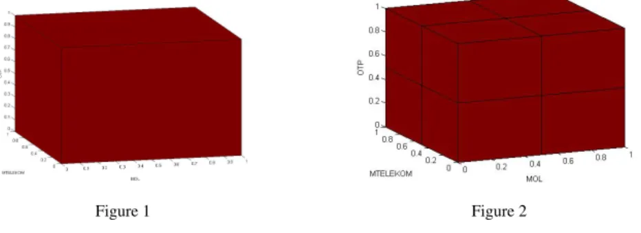
At the beginning of the algorithm in step 1 the family of setHhas been defined (see Figure 1).
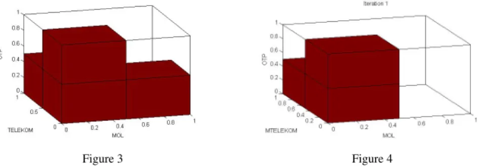
Figure 1 Figure 2
At the first iteration the procedureNewsetsin step 2(a), definesH0in the following way. First, it cuts the setH0into eight equal pieces as you see in Figure 2. After that
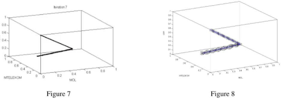
Figure 3 Figure 4
all those sets are deleted fromH0that does not contain any point from the feasible solution set of the problem. Thus the result of the procedureNewsets, the family of H0covering the feasible solution set of the given problem has been shown in Figure 3.
Figure 5 Figure 6
The main part of the algorithm starts at step 2(c). Two hundred random points are generated from the unit simplex (setS P). For each generated point either a joint decreasing direction is computed and after that a corresponding Pareto optimal solution has been identified through some iteration or it has been shown that the generated point itself is a Pareto optimal solution of the problem. After we obtained 200 Pareto optimal solutions in setF P at step 2(d)we delete those boxes that does not contain any point fromF Pat step 2(e). The result of the first iteration can be seen in Figure 4.
From the original eight boxes remains three. For these three boxes the procedure has been repeated in the second iteration. The results of iteration 3, 5 and 7 are illustrated in Figures 5, 6, and 7, respectively.
These figures illustrate the flow of our computations. Finally to illustrate the con- vergence of our method the whole Pareto optimal set was determined based on the result of [37], and compared to the result computed in the fifth iteration, see in Figure 8.
The summary of our computations are shown in the 1 whereIstands for the iteration number;BinandBout denotes the number of boxes at the beginning and at the end
Figure 7 Figure 8
of iteration, respectively. Furthermore, T(s)is the computational time of theIth iteration in seconds, whiledis the diameter of the family of sets,H.
I Bin T(s) Bout d
1 1 8 3 2−3
2 24 29 7 2−6
3 56 70 15 2−9
4 120 166 29 2−12
5 232 312 56 2−15
6 448 696 110 2−18
7 880 1429 228 2−21
Table 1
Computational results for Markowitz model using subdivision method.
The total computational time for our MATLAB implementation using a laptop with the following characteristics (processor: Intel(r) Core(TM) i3 [3.3 GHZ], RAM Memory: 4096 MB), took 2710 seconds for the subdivision algorithm for the given Markovitz model to approximate the whole Pareto optimal solution set with the ac- curacyε=2.4 10−8.
Analyzing our approximation of the Pareto optimal solution set, we can conclude that our first option is to buy OTP shares only. From the data it can be understood that this share has the biggest return (smallest loss in the financial crisis), so this solution represents the strategy when someone does not care about the risk but only about the return. From that point a line starts which represents strategies related to portfolios based on OTP and MOL shares. Clearly, there exists a breaking point where a new line segment starts. From the braking point the line lies in the interior of the simplex suggesting a portfolio based on all three selected shares.
Acknowledgement
This research has been supported by the TÁMOP-4.2.2./B-10/1-2010-0009, Hun- garian National Office of Research and Technology with the financial support of the European Union from the European Social Fund.
Tibor Illés acknowledges the research support obtained as a part time John An- derson Research Lecturerfrom the Management Science Department, Strathclyde University, Glasgow, UK. This research has been partially supported by the UK Engineering and Physical Sciences Research Council (grant no. EP/P005268/1).
References
[1] A.A. Akkele¸s, L. Balogh and T. Illés, New variants of the criss-cross method for linearly constrained convex quadratic programming.European Journal of Operational Research, 157:74–86, 2004.
[2] M.S. Bazaraa H.D. Sherali and M.C. Shetty,Nonlinear Programing Theory and Algorithms.3-rd edition, Jhon Wiley & Son Inc., New Jersey, 2006.
[3] Budapest Stock Exchange, http://client.bse.hu/topmenu/trading_
data/stat_hist_download/trading_summ_pages_dir.html Accessed: 2012. 06. 10.
[4] Zs. Csizmadia,New pivot based methods in linear optimization, and an ap- plication in petroleum industry, PhD Thesis. Eötvös Loránd University of Sciences, Budapest, Hungary, 2007.
[5] Zs. Csizmadia and T. Illés, New criss-cross type algorithms for linear com- plementarity problems with sufficient matrices. Optimization Methods and Software, 21(2):247–266, 2006.
[6] Zs. Csizmadia, T. Illés and A. Nagy, The s-monotone index selection rules for pivot algorithms of linear programming.European Journal of Operation Research, 221(3):491–500, 2012.
[7] M. Dellnitz, O. Schütze and T. Hestermeyer, Covering Pareto Sets by Multi- level Subdivision Techniques.Journal of Optimization Theory and Applica- tions, 124(1):113–136, 2005.
[8] M. Dellnitz, O. Schütze and Q. Zheng, Locating all the zeros of an ana- lytic function in one complex variable,Journal of Computational and Applied Mathematics, 138(2):325–333, 2002.
[9] G. Eichfelder, Adaptive Scalarization Methods in Multiobjective Optimiza- tion, Springer-Verlag, Berlin, Heidelberg, 2008.
[10] G. Eichfelder and T.X.D. Ha, Optimality conditions for vector optimization problems with variable ordering structures.Optimization: A Journal of Math- ematical Programming and Operations Research, 62(5):597–627, 2013.
[11] Farkas Gy., A Fourier-féle mechanikai elv alkalmazásai, (The applications of the mechanical principle of Fourier [in Hungarian]).Mathematikai és Termé- szettudományi Értesít˝o, 12:457–472, 1894.
[12] Gy. Farkas, Theorie der einfachen Ungleichungen.Journal für die Reine und Angewandte Mathematik, 124:1–27, 1902.
[13] J. Fliege, B.F. Svaiter, Steepest Descent Methods for Multicriteria Optimiza- tion, Mathematical Methods of Operations Research.Mathematical Methods of Operations Research, 51:479–494, 2000.
[14] J. Fliege, An Efficient Interior-Point Method for Convex Multicriteria Optimization Problems, Mathematical Methods of Operations Research, 31(4):825–845, 2006.
[15] F. Giannessi, G. Mastroeni and L. Pellegrini, On the Theory of Vector Opti- mization and Variational Inequalities. Image Space Analysis and Separation.
InVector Variational Inequalities and Vector Equilibria: Mathematical The- ories, editor: F. Giannessi. Series on Nonconvex Optimization and its Appli- cations, Vol.38, Kluwer, Dordrecht, 2000.
[16] D. den Hertog, C. Roos and T. Terlaky, The linear complementarity prob- lem, sufficient matrices and the criss-cross method.Linear Algebra and Its Applications, 187:1–14, 1993.
[17] T. Illés and K. Mészáros, A New and Constructive Proof of Two Basic Results of Linear Programming.Yugoslav Journal of Operations Research, 11:15–30, 2001.
[18] T. Illés and M. Nagy, A new variant of the Mizuno-Todd-Ye predictor- corrector algorithm for sufficient matrix linear complementarity problem.Eu- ropean Journal of Operational Research, 181(3):1097–1111, 2007.
[19] T. Illés, M. Nagy and T. Terlaky, Interior Point Algorithms [in Hungar- ian] (Bels˝opontos algoritmusok), pp. 1230–1297. Iványi Antal (alkotó sz- erkeszt˝o), Informatikai Algoritmusok 2, ELTE Eötvös Kiadó, Budapest, 2005.
[20] T. Illés, C. Roos and T. Terlaky, Polynomial Affine–Scaling Algorithms forP∗(κ)Linear Complementarity Problems. In P. Gritzmann, R. Horst, E.
Sachs, R. Tichatschke, editors,Recent Advances in Optimization, Proceed- ings of the 8th French-German Conference on Optimization, Trier, July 21- 26, 1996,Lecture Notes in Economics and Mathematical Systems 452, pp.
119–137, Springer Verlag, 1997.
[21] T. Illés and T. Terlaky, Pivot Versus Interior Point Methods: Pros and Cons.
European Journal of Operations Research140:6–26, 2002.
[22] E. Klafszky and T. Terlaky, The role of pivoting in proving some fundamental theorems of linear algebra.Linear Algebra and its Application151:97–118, 1991.
[23] D.T. Luc,Theory of Vector Optimization. Lecture Notes in Economics and Mathematical Systems, No. 319, Springer-Verlag, Berlin, 1989.
[24] G D. Luenberger and Y Ye,Linerar and Nonlinear Programming. Interna- tional Series in Operations Research and Management Science, Springer- Verlag, New York, 2008.
[25] H. Markowitz, The Optimalization of Quadratic Function Subject to Linear Constarint.Naval Reserch Logistic Quartely, 3(1-2):111–133, 1956.
[26] H. Markowitz, Portfolio Selection. The Journal of Finance, 7(1):77–91, 1952.
[27] H. M. Markowitz,Portfolio Selection: Efficient Diversification of Investment, Jhon Wiley and Son Inc., New York, 1959.
[28] K. Miettinen,Nonlinear Multiobjective Optimization. International Series in Operations Research and Management Science, Springer US, 1998.
[29] K. G. Murty,Linear Complementarity, Linear and Nonlinear Programming.
Heldermann Verlag, Berlin, 1988.
[30] V. Pareto,Cours D’Économie Politique. F. Rouge, Lausanne, 1896.
[31] Prékopa A.,Lineáris programozás I.. Bolyai János Matematikai Társulat, Bu- dapest, 1968.
[32] A. Prékopa, A Very Short Introduction to Linear Programming.RUTCOR Lecture Notes2-92, 1992.
[33] C. Roos, T. Terlaky and J-Ph. Vial,Theory and Algorithms for Linear Opti- mization: An Interior Point Approach. Wiley-Interscience Series in Discrete Mathematics and Optimization, John Wiley & Sons., 1997.
[34] S. Schäffler, R. Schultz and K. Weinzierl, A Stochastic Method for the Solu- tion of Unconstrained Vector Optimization Problems.Journal of Optimaliza- tion Theory and Application, 114(1):112–128, 2002.
[35] A. Schrijver, Theory of Linear and Integer Programming, John Wiley and Sons Inc., New York, 1986.
[36] T. Terlaky, A convergent criss–cross method.Math. Oper. und Stat. Ser. Op- timization16(5):683–690, 1985.
[37] J. Vörös, Portfolio analysis – An analytic derivation of the efficient portfolio frontier.European Journal of Operational Reserch, 23(3):294–300, 1986.