Tree decompositions of graphs and their eﬀect on algorithmic complexity

(1)

Tree decompositions of graphs and their effect on algorithmic complexity

Dániel Marx

Institute for Computer Science and Control, Hungarian Academy of Sciences

(MTA SZTAKI)

Budapest

2019

(2)

(3)

CHAPTER 1 Introduction

A wide range of application areas require efficient algorithmic solutions for combinatorial problems.

The theory of NP-hardness tells us that we cannot expect optimal polynomial-time algorithms for many of the optimization problems that arise in practice. While in these cases we cannot hope for efficient algorithms tackling the problem in its full generality, it may still be possible that an algorithm is provably efficient on certain special cases of practical or theoretical relevance. A large part of the theoretical research on algorithms can be seen as trying to identify favorable properties of the input instance that allow efficient algorithms.

Perhaps the most well-studied such property is the concept of decomposability: the problem instance can be recursively split into smaller parts such that the solutions of the smaller parts can be combined into a solution of the whole instance. The exact meaning of decomposability depends on the problem domain, but typically it means the existence of small separators that break the problem into fairly independent parts that only interact via the separator. For algorithmic problems that are explicitly defined on graphs (or perhaps there is a natural definition of a graph that can be associated with the problem instance), the notion oftreewidthappears to be a very useful concept in formalizing decomposability. Informally speaking, treewidth measures how close a graph is to being a tree: graphs of small treewidth are similar to a tree with each node being replaced by a small graph. While the formal definition of treewidth is technical, it models very faithfully the requirements that make the algorithmic paradigm “split on small separators and recurse” work and its mathematical naturality is further evidenced by the fact that it was independently discovered in equivalent formulations at least three times [28, 135, 207].

The overarching theme of this dissertation is the quest for understanding how structural parameters such as treewidth and its variants make algorithmic problems provably more tractable. The results presented here include both algorithms (upper bounds on the running time) and complexity result (lower bounds on the running time). The results answer three different types of fundamental questions. First, given a certain algorithmic problem, we can ask if there is an efficient solution that works on instances that have low treewidth. In other words, we would like to know if treewidth helps resolving the problem in any way.

(6)

Does low value of treewidth (or a related measure) make it possible to solve certain type of problems efficiently?

After establishing that treewidth is a useful parameter, we would like to quantify this statement by understanding how exactly the running time can depend on treewidth. That is, we would like to have optimal algorithms that exploit treewidth as much as possible. Besides presenting the optimal algorithm, one needs to argue that the dependence on treewidth cannot be improved. Thus we need complexity results ruling out any possible improvement.

What is the best possible dependence on treewidth (or a related measure) that can be achieved for a given problem?

Finally, if we know exactly how treewidth influences the complexity of a problem, it is natural to ask if there is another graph property (perhaps some variant of treewidth) that decreases the complexity of the problem in a similar way.

Is bounded treewidth (or a related measure) the only graph-theoretical property that decreases the complexity of a given problem?

While questions of such form may sound very open ended, it is possible to define frameworks formalizing these questions and to give completely exhaustive answers [68, 69, 77, 123, 127, 154]. In particular, in some cases it is possible to prove “dichotomy theorems” showing formally that only the bounded-treewidth special cases are tractable, and every otherspecial case is hard.

The goal of the rest of this introduction is twofold. It briefly goes over basic concepts that will be needed in the later chapters (such as treewidth and constraint satisfaction problems), serving as a shared prelimianaries section to avoid repeating the introduction of the same defininions all over again in each chapter. Moreover, we use this introduction to put the main results of the dissertation into context and briefly explain how they improve on what was known earlier. Here we highlight only a selection of results and state them in an informal manner; for formal statements of all the results, the reader is referred to the appropriate chapters.

Many of the results presented in the dissertation are complexity lower bounds. Of course, these results are all conditional lower bounds: as we cannot rule out P=NP at the moment, in principle it is possible that every problem considered here can be solved efficiently and these lower bounds are irrelevant. As it is customarily done in theoretical computer science, we assume a complexity hypothesis (such as P6=NP) and we prove the lower bounds under this assumption. Section 1.1 introduces these assumptions. The framework of parameterized complexity and fixed-parameter tractability is used explicitly or implicitly in most of the results; Section 1.2 gives a brief overview of these topics. Section 1.3 defines treewidth and introduces related graph-theoretical notions.

Section 1.4 introduces one of the main application domains for our results: Constraint Satisfaction Problems (CSPs). Section 1.5 gives a brief overview of some basic notions of database theory relevant for our results. For reference, Section 1.6 summarizes the publication venues where the results presented in the different chapters of the dissertation originally appeared.

(7)

1.1. COMPLEXITY ASSUMPTIONS 7

1.1 Complexity assumptions

The widely-believed complexity assumption P 6= NP has immense explanatory power: via the theory of NP-completeness, this assumption explains why important combinatorial problems are not polynomial-time solvable. The use of the P6=NP hypothesis goes beyond explaining the hardness of finding optimal solutions. In recent decades, the field of inapproximability has seen enormous progress and very strong lower bounds on polynomial-time approximabilty can be obtained based on the P6=NP hypothesis [18, 86, 137].

However, there are important complexity lower bounds that currently are not known to be provable from P6=NP, requiring a stronger complexity assumption. For example, in the field of inapproximability, the Unique Games Conjectures introduced by Khot [162] allows proving tight lower bounds on the approximation ratio that match the best known algorithms [53, 131, 162, 163].

In the field of parameterized and exact computation, the P 6=NP assumption only tells us that NP-hard problems do not admit polynomial-time algorithms, but does not say anything about the existence of subexponential-time algorithms. That is, it is still possible that there are much faster algorithms for NP-hard problems than what we know today: for example, as far as we know, the P6=NP assumption does not rule out algorithms with running time 2^n/10000, or 2ⁿ^1/100, orn^logⁿ, or evenn^{log log}ⁿ for an NP-hard problem such as 3SAT withnvariables.

The Exponential-Time Hypothesis (ETH), formulated by Impagliazzo, Paturi, and Zane [145,146], makes the assumption P 6= NP more quantitative: informally, it not only tells us that NP-hard problems do not have polynomial-time algorithms, but it posits that NP-hard problems really require exponential time and cannot be solved in subexponential time. The formal statement of the ETH is somewhat technical and for most applications it is more convenient to use the following assumption instead, which is an easy consequence of the ETH:

Hypothesis 1.1 (Consequence of the ETH, Impagliazzo, Paturi, and Zane [145, 146]). 3SATwith nvariables cannot be solved in time 2^o(n).

3SATis the fundamental satisfiability problem where, given a Boolean formula in conjunctive normal form with at most 3 literals in each clase (e.g.,(x1∨x¯3∨x5)∧(¯x1∨x2∨x3)∧(¯x2∨x3∨x4)), the task is to decide whether a satisfying assignment exists. For completeness, let us recall the formal statement of the ETH, of which Hypothesis 1.1 is an easy consquence. Letsk be the infinum of all real numbersδ for which there exists an O(2^δn) time algorithm for k-SAT. Then the ETH is the assumption that s_k > 0 for every k ≥ 3. It is easy to show that this assumption implies Hypothesis 1.1, hence if we can show that some statement would refute Hypothesis 1.1, then it would refute the ETH as well.

Hypothesis 1.1 rules out the existence of algorithms that are subexponential in the number nof variables. But the number m of clauses in a 3SATinstance can be up to cubic in the number of variables, thus the length of the instance can be much larger than O(n). Therefore, Hypothesis 1.1 does not rule out the existence of algorithms that are subexponential in the length of the instance:

it could be potentially the case that all the really hard instances of 3SAT have, say,Ω(n²) clauses, hence a 2^o(

√m) algorithm would be still compatible with Hypothesis 1.1. Impagliazzo, Paturi and Zane [146] showed that this is not the case: the Sparsification Lemma implies that, for the purposes of Hypothesis 1.1,3SAT remains hard already when restricted to instances with a linear number of clauses. With the Sparsification Lemma, the following stronger assumption follows from Hypothesis 1.1:

Hypothesis 1.2 (Consequence of the ETH + Sparsification Lemma, Impagliazzo, Paturi, and Zane [146]). 3SAT with n variables and m clauses cannot be solved in time 2^o(n+m).

(8)

This stronger assumption turns out to be very useful to prove lower bounds for other problems.

Reductions from 3SATto other problems typically create instances whose size depend not only on the numbernof variables, but also on the number mof clauses, hence it is important to have lower bounds on3SAT in terms of bothnand m.

Despite the usefulness of the ETH, there are complexity lower bounds that seem to be beyond the reach of what can be proved as a consequence of this hypothesis. Impagliazzo, Paturi, and Zane [146]

proposed an even stronger assumption on the complexity of NP-hard problems: the so-called Strong Exponential-Time Hypothesis (SETH). Using the notation introduced above, the SETH assumes that limk→∞sk= 1. The following consequence of the SETH is a convenient formulation that can be used as a starting point for lower bounds on other problems:

Hypothesis 1.3 (Consequence of the SETH, Impagliazzo, Paturi, and Zane [146]). SAT with n variables and m clauses cannot be solved in time (2−)ⁿ·m^O(1) for any >0.

Intuitively, Hypothesis 1.3 states that there is no better algorithm forSAT than the brute force search of trying each of the2ⁿ possible assignments. Note that hereSATis the satisfiability problem with unbounded clause length. For fixed clause length, algorithms better than2ⁿ are known: for example, the best known algorithms for 3SATand 4SAThave running times1.308ⁿ and1.469ⁿ, respectively [138]. The SETH states that the base of the exponent has to get closer and closer to 1 as the clause length increases, and it is not possible to have an algorithm with base2−that works for arbitrary large clause length.

It is important to note that there is no known analogue of the Sparsification Lemma for the SETH. That is, we cannot assume that the hard instances stipulated by Hypothesis 1.3 have only a linear number of clauses: for all we know, the number of clauses can be exponential in the number n of variables. This severly limits the applicability of lower bounds based on the SETH as any reduction from theSATinstance would create instances whose sizes are potentially exponentially large in n. Nevertheless, the SETH has found applications in parameterized complexity, where instead of giving a lower bound on how the running time has to depend on the instance or solution size, we want to understand how it depends on some other parameter. Chapter 2 contains a selection of such results, giving tight lower bounds on how the running time has to depend on treewidth.

The results presented in this chapter were the first such tight lower bounds on parameterization by treewidth, inspiring many subsequent results of this form [38, 70, 72, 76, 91, 151, 152]. In recent years, the SETH has been successfully used to give lower bounds for polynomial-time solvable problems, for example, by showing that the textbook O(n²) dynamic programming algorithm forEdit Distance cannot be significantly improved: it cannot be solved in time O(n²⁻) for any > 0, unless the SETH fails [22, 43]. Many other tight results of this form can be found in the recent literature under the name “fine-grained complexity” [1–3, 22, 39, 40, 43, 44, 202, 210, 232].

The ETH and the SETH are stronger assumptions that the P6= NP hypothesis and perhaps not as widely accepted in the research community. Thus one may wonder about the meaning of conditional lower bounds based on them. First, by now the ETH is fairly well accepted in the research community and has been used as the starting point to prove lower bounds for numerous problems (e.g., [16,73,80,104,106,175]). Indeed, despite decades of research on3SAT, there is no sign whatsoever that subexponential algorithms would be possible and in fact minor improvements of the base of the exponential function in the running time required considerable efforts [138, 139, 148, 170, 173, 193].

The SETH is a much more ambitious proposition and there is less evidence supporting its validity.

Still, the explanatory power of this hypothesis has been used in a large number of recent research results and obtaining conditional lower bounds based on it has become a mainstream research direction. Regardless of what the reader may think of the validity of the SETH, the following point of view should clarify why results of this form are still valuable. A conditional lower bound showing

(9)

1.2. PARAMETERIZED COMPLEXITY 9 that “a better algorithm for problem X would violate the SETH” shows that in order to improve the algorithm for problem X, one needs to be able to deal with theSATproblem in its full generality. It is not the particular difficulties of problem X that needs to be better understood to improve the running time: improvements are prevented by the lack of better understanding of satisfiability itself.

Thus it can be argued that instead of focusing on problem X, one should better focus on the more fundamental question of improvingSAT algorithms directly, because this is what improvements on problem X would eventually achieve. In other words, the conditional lower bound closes the question

“Are there better algorithms for problem X?” by saying one should not directly work on this question until the validity of the SETH is resolved one way or the other.

1.2 Parameterized complexity

Classical complexity theory expresses the running time of an algorithm as a univariate function of the size nof the input. The main conceptual idea of parameterized complexity is to introduce additional parameters and to express the running time as a multivariate function of the input size and these parameters. The goal is to find algorithms where the exponential growth of the running time is restricted to these parameters, while the running time depends only polynomially on the size of the input. If we have an application where the parameters can be assumed to be small, then such an algorithm can be efficient even for large input sizes.

Formally, we associate an integer parameter k with each input instance of the problem and we say that the problem isfixed-parameter tractable (FPT) if the problem can be solved in timef(k)n^c, where f is an arbitrary computable function depending only on kand cis a constant (independent ofk). If the functionf(k) is a moderately growing exponential function and dis not too large, then an FPT-time algorithm can be efficient for applications wherek is small. For example, an algorithm with running time, say,O(1.2852^k+kn) fork-Vertex Cover[61] is feasible fork= 40, since in this case the term1.2852^k is only about 22000.

The classical work of Downey and Fellows [87] summarized the results of the field up to 1999, with more recent monographs [74, 88, 102, 197] providing an introduction to the enormous progress that happened since then. In the past 20 years, the parameterized complexity community identified hundreds of NP-hard problems that are fixed-parameter tractable with natural parameterizations.

The most studied graph-theoretic examples include finding a cycle of length exactlyk [13, 165, 231], finding a vertex cover of sizek[5,61,62,82,129,220], findingkvertex disjoint triangles in a graph [169], and various problems parameterized by the treewidthk of the input graph (cf. [17, 32]). Systematic search efforts were undertaken to find fixed-parameter tractable problems in various problem domains such as artificial intelligence [118], computational biology [50, 120, 182], and geometric problems [111, 181, 191]. The first results were obtained by ad hoc techniques, but (especially in the past decade) there have been intensive efforts to understand the methods used for obtaining FPT-time algorithms, turning them into general techniques. Currently, we have an impressive toolbox of algorithmic techniques at our disposal (cf. [74, 144, 218, 219]). However, many problems resisted all algorithmic techniques and no FPT-time algorithm is known for them. The theory of W[1]-hardness is the parameterized-complexity analog of NP-hardness, and can be used to give strong theoretical evidence that a problem is not fixed-parameter tractable. Although technically more difficult to prove than NP-hardness, the W[1]-hardness of numerous problems has been shown in the literature. Intuitively,Cliqueis W[1]-complete and W[1]-hard means that it is at least as hard asCliquefrom the viewpoint of fixed-parameter tractability. As the current dissertation does not present any W[1]-hardness proofs (all the lower bounds are based on the ETH or the SETH), the formal definition of W[1]-hardness will not be important.

(10)

The parameter kof the instance can be any well-defined measure of the instance. For a given algorithmic problem, one can define different natural parameters, leading to different parameterizations of the same problem. It may very well be the case that the same problem is fixed-parameter tractable with one parameterization and W[1]-hard with some other. For optimization problems (for example, finding a clique, dominating set, path etc. of maximum/minimum size), the most natural parameterization is by the size of the solution we are looking for. That is, we assume that the input instance contains a target number k, and the task is to find a solution of size at least/at most k in time f(k)nÔ(1). But there are many other potential parameters one can define. The input may already contain different values that one can choose as the parameter: for example, Partial Vertex Cover asks for the selection ofk vertices that cover at leastèdges — one can parameterize by eitherkorìn this problem. The parameter can be a measure of some aspect of the input instance: the maximum degree or treewidth in a graph problem, the dimension of the point set in a geometric problem, the alphabet size or the length of the strings in a pattern matching problem, or the domain size of the variables in a constraint satisfaction problem. Even for a single problem, one can discover a rich and nontrivial complexity landscape by considering different (combinations of) parameters [41, 189].

1.3 Graphs and hypergraphs

A large part of the dissertation deals with graphs and graph-like structures. We provide a brief overview of the main notions here, including the definition of treewidth, which will be used in many of the chapters. For ease of readability, some of the definitions will be repeated later. For more background on graph theory, the reader is referred to, e.g., the text book of Diestel [85].

Let G be a graph with vertex set V(G) and edge set E(G). A graph G⁰ is a subgraph of G if V(G⁰)⊆ V(G) andE(G⁰) ⊆E(G). For a subset V⁰ ⊆ V(G), the subgraph G⁰ =G[V⁰] of G is called a subgraph induced byV⁰ ifE(G⁰) ={uv∈E(G)|u, v∈V⁰} andV(G⁰) =V⁰. By N(u) we denote the (open) neighborhood of u in graphG, that is, the set of all vertices adjacent tou and by N[u] =N(u)∪ {u}. Similarly, for a subset D⊆V(G), we define N[D] =∪v∈DN[v].

Treewidth. Atree decomposition of a graphGis a pair (B, T)whereT is a tree andB={B_t| t∈V(T)}is a collection of subsets of V(G)such that:

• S

t∈V(T)Bt=V(G),

• for each edge xy∈E(G),{x, y} ⊆Bt for somet∈V(T);

• for each x∈V(G) the set {t|x∈Bt} induces a connected subtree ofT.

The setsBt are called the bags of the decomposition. Sometimes it will be convenient for us to view the trees in a tree-decomposition as being rooted and directed from the root to the leaves. For a nodetin a (rooted) treeT = (V(T), E(T)), we let T_t be the subtree rooted att, that is, the induced subtree of T whose vertex set is the set of all vertices reachable from t.

Thewidth of the tree decomposition ismaxt∈V(T){|B_t| −1}. The treewidth of a graphGis the minimum width over all tree decompositions ofG. We denote bytw(G)the treewidth of graphG. It is known that tw(G)≤1if and only if G is a forest (has no cycles). If in the definition of treewidth we restrict the treeT to be a path then we get the notion ofpathwidth and denote it by pw(G). By definition, we have that tw(G) ≤pw(G), but it is known that pathwidth cannot be bounded by any function of treewidth: if Gis a complete binary tree width 2k+ 1levels, thentw(G) = 1and pw(G) =k.

(11)

1.3. GRAPHS AND HYPERGRAPHS 11 We say that a class G of graphs is ofbounded treewidth if there is aksuch thattw(G)≤kfor all G∈ G. We use a similar terminology for other graph invariants.

Computing the treewidth of a given graph is known to be NP-hard [17], but for every fixedk≥1, there is a linear-time algorithm for finding a decomposition of widthk, if exists [31]. That is, finding a decomposition of widthk is fixed-parameter tractable. In polynomial time, one can compute a tree decomposition of widthO(tw(G)·p

tw(G)) [15].

There are well-known classes of graphs that have small treewidth, for example series-parallel and outerplanar graphs have treewidth at most 2, and every planar graph onnvertices has treewidth O(√

n) [30, 33]. One can argue that real-word graphs that exhibit some hierarchical structure should have treewidth much smaller than the number of vertices [132, 178, 226]. For such graphs, algorithms exploiting tree decompositions can explain the tractability of various problems.

Given a tree decomposition of widthk, the standard technique of dynamic programming over a tree decomposition can result in algorithms with running time f(k)·nfor various fundamental combinatorial problems such asIndependent Set,Vertex Cover, Dominating Set,Hamilto- nian Cycle,3-Coloring, etc. Even though the process of designing such a dynamic programming algorithm is fairly standard, one still needs to define partial subproblems in a problem-specific way, sometimes resulting in long and cumbersome proofs. In many cases, Courcelle’s Theorem [67] autom- atizes this process: as a powerful and far-reaching generalization of simple dynamic programming algorithms, it shows thatevery decision problem that can be described as a logical formula φ in Extended Monadic Second Order Logic can be solved in timef(φ, k)·non graphs of treewidth at most k.

While Courcelle’s Theorem immediatelly gives anf(k)·ntime algorithm on graphs of treewidth k for, say, 3-Coloring, it does not give good bounds on the growth rate of the function f(k).

Often, problem-specific techniques can deliver algorithms with better bounds on f(k). While for Independent Setit is fairly straightforward to obtain an algorithm with running time2^k·nÔ(1), the 3^k·nÔ(1)time algorithms forDominating Setrequired the application of the nontrivial Fast Subset Convolution technique [29, 227] and the firstc^k·nÔ(1) time algorithms for Hamiltonian Cycle was made possible only with the Cut & Count technique [76] and the rank-based approaches [34, 75].

Given that for some problems new techniques were necessary to improve the dependence on treewidth and for others essentially no progress was made, it is natural to ask what the best possible dependencef(k) on treewidth is. The results in Chapter 2 answer precisely this question: they show that, assuming the SETH, for several basic problems (such asIndpendent Setand 3-Coloring) the best known algorithm has essentially optimal dependence on treewidth, up to anterm in the base of the exponential function. These results closed the question of whether further improvements can be expected for these problems. At the time of publication of the conference version of this work [174] in SODA 2011, these results were the first results proving such tight lower bounds for parameterization by treewidth; inspired by this work, similar results were published later by other authors [38, 70, 72, 76, 91, 151, 152].

Hypergraphs. In a graph, each edge connects two vertices, representing a relation of arity two such as “connected”, “adjacent”, or “conflicts with,” etc. In some cases, the natural representation of a problem requires expressing relations of higher arity, for example, expressing that certain items appear in groups. Hypergraphs are natural generalizations of graphs, allowing hyperedges containing more than two vertices. Formally, a hypergraph is a pair H = (V(H), E(H)), consisting of a set V(H) of vertices and a set E(H) of nonempty subsets ofV(H), thehyperedges ofH.

For a hypergraphHand a setX ⊆V(H), thesubhypergraph ofH induced byXis the hypergraph H[X] = (X,{e∩X |e∈E(H)withe∩X 6=∅}). We let H\X=H[V(H)\X]. Theprimal graph

(12)

of a hypergraph H is the graph

H= (V(H),{{v, w} |v6=w, there exists an e∈E(H) such that{v, w} ⊆e}).

A hypergraphH isconnected ifH is connected. A setC ⊆V(H) isconnected (in H)if the induced subhypergraphH[C]is connected, and aconnected component of H is a maximal connected subset of V(H). A sequence of vertices ofH is a pathof H if it is a path of H.

Let us generalize the notion of tree decomposition and treewidth to hypergraphs. A tree decomposition of a hypergraphH is a pair (B, T) where T is a tree andB={B_t|t∈V(T)} is a collection of subsets of V(H) such that:

• S

t∈V(T)B_t=V(H),

• for each hyperedge e∈E(H), we have e⊆B_t for some t∈V(T);

• for each x∈V(H) the set {t|x∈Bt} induces a connected subtree ofT.

The setsB_t are called thebags of the decomposition. Thewidth of a tree-decomposition(T,B) is max

|B_t|

t∈V(T)} −1. The treewidth tw(H) of a hypergraphH is the minimum of the widths of all tree-decompositions of H. It is well-known and easy to see thattw(H) = tw(H) for allH.

1.4 Constraint Satisfaction Problems

Constraint satisfaction is a general framework that includes many standard algorithmic problems such as satisfiability, graph coloring, database queries, etc. A constraint satisfaction problem (CSP) consists of a set V of variables, a domainD, and a set C of constraints, where each constraint is a relation on a subset of the variables. The task is to assign a value fromD to each variable in such a way that every constraint is satisfied (see Definition 1.4 below for the formal definition). For example, 3SAT can be interpreted as a CSP instance where the domain is {0,1} and the constraints in C correspond to the clauses (thus the arity of each constraint is 3). Another example is vertex coloring, which can be interpreted as a CSP instance where the variables correspond to the vertices, the domain corresponds to the set of colors, and there is a binary “not equal” constraint corresponding to each edge. Notice that the domain size can be arbitrarily large in the CSP instances arising from vertex coloring (as the coloring problem might involve any number of colors). In the this dissertation, we think of the domain as a set whose size is not a fixed constant, but can be be arbitrarily large. This viewpoint is natural in the context of various database query and artificial intelligence applications, where in fact that domain size is usually much larger than the number of variables [118, 211].

Basic definitions. We briefly recall some terminology related to CSP. For more background, see, for example, [96, 122].

Definition 1.4. An instance I of aconstraint satisfaction problemis a tripleI = (V, D, C), where:

• V is a set of variables,

• D is a domain of values,

• C is a set of constraints, {c₁, c₂, . . . , c_q}. Each constraint c_i∈C is a pairhs_i, R_ii, where:

– s_i is a tuple of variables of length m_i, called the constraint scope,and – Ri is anmi-ary relation over D, called theconstraint relation.

(13)

1.4. CONSTRAINT SATISFACTION PROBLEMS 13 For each constrainths_i, R_ii the tuples ofR_i indicate the allowed combinations of simultaneous values for the variables in s_i. The length m_i of the tuple s_i is called the arity of the constraint.

We allow repeated variables in the scopesi, but this does not make the problem more general and can be usually ignored. A solution to a constraint satisfaction problem instance is a function f from the set of variablesV to the domain D of values such that for each constraint hs_i, R_ii with si = (vi1, vi2, . . . , vim), the tuple (f(vi1), f(vi2), . . . , f(vim)) is a member of Ri. In the decision version of CSP, we have to decide if a solution for the given instanceI exists. Observe that there is a polynomial-time algorithm deciding whether a given assignment for an instance is a solution.

The primal graph(or Gaifmann graph) of a CSP instanceI = (V, D, C) is a graphGwith vertex set V, wherex, y ∈V form an edge if and only if there is a constraint hs_i, R_ii ∈C with x, y∈s_i. For a classG of graphs, we denote by CSP(G) the problem restricted to instances where the primal graph is inG. Note that this definition does not make any restriction on the constraint relations: it is possible that every constraint has a different constraint relation.

The hypergraph of an instanceI = (V, D, C)hasV as its vertex set and for every constraint inC a hyperedge that consists of all variables occurring in the constraint. For a classHof hypergraphs, we let CSP(H) be the class of all instances whose hypergraph is contained inH.

We say that an instance isbinary if each constraint relation is binary, that is,mi = 2for every constraint¹. It can be assumed that the instance does not contain two constraintshs_i, Rii,hs_j, Rji withs_i =s_j, since in this case the two constraints can be replaced by the constraint hs_i, R_i∩R_ji.

Representation of the constraints. In the input, the relation in a constraint is represented by listing all the tuples of the constraint. We denote bykIkthe size of the representation of the instance I = (V, D, C). For binary constraint satisfaction problems, we may assume that kIk=O(V²D²); by the argument in the previous paragraph, we may assume that there areO(V²)constraints and each constraint has a representation of length O(D²). Furthermore, it can be assumed that|D| ≤ kIk;

elements ofDthat do not appear in any relation can be removed.

If constraints of larger arity are also allowed in the input, we have to be more careful and precise in describing how the constraints are represented and how this representation contributes to the input size. Throughout this dissertation, we assume that the constraints are specified by explicitly enumerating all possible combinations of values for the variables, that is, all tuples in the relation R. Consequently, we define the size of a constraint c = h(v₁, . . . , vk), Ri ∈ C to be the number kck=k+k· |R|. Thesize of an instance I = (V, D, C) is the numberkIk=|V|+|D|+P

c∈Ckck.

Of course, there is no need to store a constraint relation repeatedly if it occurs in several constraints, but this only changes the size by a polynomial factor.

Let us make a few remarks about this explicit representation of the constraints. There are important special cases of constraint satisfaction problems where the constraints are stored implicitly, which may make the representation exponentially more succinct. Examples include Boolean satisfiability, where the constraint relations are given implicitly by the clauses of a formula in conjunctive normal form, or systems of arithmetic (in)equalities, where the constraints are given implicitly by the (in)equalities. However, our representation is the standard “generic” representation of constraint satisfaction problems in artificial intelligence (see, for example, [81]). An important application where the constraints are always given in explicit form is the conjunctive query containment problem, which plays a crucial role in database query optimization. Kolaitis and Vardi [166] observed that it can be represented as a constraint satisfaction problem, and the constraint relations are given explicitly as part of one of the input queries. A related problem from database systems is the problem of evaluating conjunctive queries (see Section 1.5 below). Here the constraint relations represent the

1It is unfortunate that while some communities use the term “binary CSP” in the sense that each constraint is binary (as does this dissertation), others use it in the sense that the variables are 0-1, that is, the domain size is 2.

(14)

tables of a relational database, and again they are given in explicit form. The problem of characterizing the tractable structural restrictions of CSP has also been studied for other representations of the instances: one can consider more succinct representations such as disjunctive formulas or decision diagrams [58] or less succinct representations such as truth tables [187]. As the choice of representation influences the size of the input and the running time is expressed as a function of the input size, the choice of representation influences the complexity of the problem and the exact tractability criterion.

Complexity classifications. Due to its generality, solving constraint satisfaction problems is NP-hard if we do not impose any additional restrictions on the possible instances. Therefore, the main goal of the research on CSP is to identify tractable classes and special cases of the general problem. The theoretical literature on CSP investigates two main types of restrictions. The first type is to restrict the constraint language, that is, the type of constraints that is allowed. This direction was initiated by the classical work of Schaefer [212] and was subsequently pursued in, e.g., [45,46,49,96,156]. Recently, as a major breakthrough, Bulatov [47] and Zhuk [234] independently characterized the complexity of every CSP problem with a fixed constraint language, resolving a long-standing open problem raised by Feder and Vardi [96]. Significant progress was made on the complexity of the optimization versions of the problem as well [79, 168, 224].

The second type is to restrict the structure induced by the constraints on the variables. The goal is to understand what structural properties of the CSP instance can make the problem easier.

The first question is to understand which graphs make CSP polynomial-time solvable. We have to be careful with the formalization of this question: if G is a graph withk vertices, then any CSP instance with primal graph G can be solved in time n^O(k) by brute force. Therefore, restricting CSP toany fixed graphGmakes it polynomial-time solvable. The real question is which classesof graphs make the problem polynomial-time solvable: using the definitions introduced above, which classes G of graphs make CSP(G) polynomial-time solvable? Freuder [108] observed that if the treewidth of the primal graph isk, then CSP can be solved in time n^O(k). Thus if G has bounded treewidth, then CSP(G) is polynomial-time solvable. Quite surprisingly, the converse is also known to be true: it follows from the work of Grohe, Schwentick, and Segoufin [123, 127] that whenever G is any recursively enumerable class of graphs with unbounded treewidth, then CSP(G) is not polynomial-time solvable, unless FPT=W[1].

By this result of Grohe, Schwentick, and Segoufin, bounded treewidth is the only property of the primal graph that can make the problem polynomial-time solvable. However it does not rule out the possibility that there is some structural property that may enable us to solve instances significantly faster than the treewidth-based algorithm of [108], that is, for some classGof graphs with unbounded treewidth, CSP(G) could be solved in timen^f^(k) wherekis the treewidth of the primal graph andf is a slowly growing function such as√

korlogk. The main result of Chapter 3 is that this is not possible;

then^O(k)-time algorithm is essentially optimal for every class of graphs, up to anO(logk)factor in the exponent. It follows as consequence of this result is that, assuming the ETH, there is nof(k)n^o(k/^log^k) time algorithm for the graph-theoretic problem Partitioned Subgraph Isomorphism, wherekis the number of edges of the pattern to be found and f is an arbitrary computable function. This lower bound turned out be a very useful starting point for proving almost tight lower bound of this form for several other W[1]-hard parameterized problems in different domains. As there is no other technique currently that would give bounds of such tightness, its use has become a standard techique that was invoked several times (e.g., [35–37, 42, 68, 71, 92, 94, 128, 155, 158, 177, 190, 203]).

Large arities. For binary CSP instances, the primal graphGcompletely describes the structure induced by the constraints. But if there are constraints of higher arity, then the primal graph loses information. For example, by looking at the primal graph only, we cannot tell whether the instance contains ^k₂

binary constraints on kvariables or just a single k-ary constriant on all the variables:

(15)

1.4. CONSTRAINT SATISFACTION PROBLEMS 15 the primal graph is a complete graph onkvertices in both cases. Thus the hypergraphH of the CSP instance contains more information than the primal graphG, hence classifying the complexity of CSP(H) for every class H of hypergraphs gives a more refined classification than classifying CSP(G) for every classG of graphs.

If a class Hof hypergraphs has bounded arity (i.e., there is an integer csuch that every edge of every hypergraph in H has size at most c), then the classification for binary CSPs essentially goes through, and it follows that bounded treewidth of the hypergraph classH is the only property that makes the problem polynomial-time solvable. However, the situation significantly changes ifH has unbounded arity. Consider for example the classH₁ containing every hypergraph where there is an edge that covers every vertex. Now the primal graph of eachH ∈ H₁ is a complete graph, thus H₁ does not have bounded treewidth. But CSP(H₁) is polynomial-time solvable: as every hypergraph in H₁ contains an edge covering every vertex, every instance of CSP(H₁) contains a constraintc involving every variable. Thus all we need is going through the satisfying assignments of constraintc and check whether one of them satisfies every other constraint (recall that we have assumed above that constraints are represented in the input by explicitly listing every assignment that satisfies it). Thus bounded treewidth of the hypergraph classH is not the right tractability criterion for characterizing the polynomial-time solvable cases of CSP(H) and the situation seems to be much more complicated. As a side note, one could say that the tractability of CSP(H₁) is only an artifact of the assumption that the constraints are represented by listing every satisfying assignment. However, as we shall see in Section 1.5, this assumption is very natural in the context of database queries, and the original motivation for this line of research was studying applications in database theory.

Generalizing the simple example ofH₁ in the previous paragraph, it was shown that there is a notion of acyclicity for hypergraphs that makes the problem polynomial-time solvable [27, 95, 233].

Generalizing acyclicity, Gottlob et al. [115–117] introduced the notion ofhypertree widthand showed that CSP(H) is polynomial-time solvable if H has bounded hypertree width. Adler et al. [8]

introducedgeneralized hypertree width,but this notion does not deliver new polynomial-time solvable cases of CSP(H): it is known thatH has bounded hypertree width if and only if it has bounded generalized hypertree width.

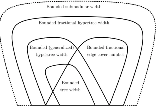
Chapter 4 introduces a the notion of bounded fractional edge cover numberand shows that if Hhas this property, then CSP(H) is polynomial-time solvable. As this property is incomparable to bounded hypertree width, it gives new tractable classes that were not known before. Chapter 5 introduces fractional hypertree width as a common generalization of fractional edge covers and hypertree width. It is shown that if Hhas bounded fractional hypertree width, then CSP(H) is polynomial-time solvable, making this property the currently known most general structural property that makes CSP(H) polynomial-time solvable. Figure 1.1 shows some of the known tractable hypergraph properties (note that the elements of this Venn diagram are sets of hypergraphs; e.g., the set “bounded treewidth” contains every setHof hypergraphs with bounded treewidth). All the inclusions in the figure are known to be proper.

Currently it is not known if there is any hypergraph classHwith unbounded fractional hypertree width that make CSP(H) polynomial-time solvable. However, if we consider a weaker form of tractability, then we can obtain algorithms for some classes with unbound fractional hypertree width.

Instead of asking for a polynomial-time algorithm, we can ask if the problem is fixed-parameter tractable parameterized by the numberk of variables, that is, there is an algorithm with running timef(k)n^O(1) for some functionf. This question is very natural in settings where the number of variables is small, but the domain size is large, making the size of the relations and the total input size much larger than the number of variables. Chapter 6 introduces the notion of submodular width and shows that if Hhas is a class of hypergraphs with bounded submodular width, then CSP(H) is

(16)

tree width

edge cover number Bounded fractional hypertree width

Bounded fractional hypertree width

Bounded (generalized)

Bounded

Bounded submodular width

Figure 1.1: Hypergraph properties that make CSP tractable. Bounded submodular width makes the problem fixed-parameter tractable, while all the othe properties make the problem polynomial-time solvable.

fixed-parameter tractable parameterized by the numberk of variables, with a functionf(k)in the running time that is double-exponential ink. Conversely, Chapter 6 shows that ifH has unbounded submodular width, then CSP(H) is not fixed-parameter tractable parameterized by the number of variables, unless the ETH fails. Thus we get a complete characterization of hypergraph classes that make CSP fixed-pararameter tractable.

1.5 Database queries

Evaluation of conjunctive queries (or equivalently, Select-Project-Join queries) is one of the most basic and most studied tasks in relational databases. A relational database consists of a fixed set of relations. A conjunctive query defines a new relation that can be obtained as first taking the join of some relations and then projecting it to a subset of the variables. As an example, consider a relational database that contains three relations: enrolled(Person,Course,Date), teaches(Person,Course,Year), parent(Person1,Person2). The following query Qdefines a unary relation ans(P) with the meaning that “P is enrolled in a course taught by her parent.”

Q:ans(P)←enrolled(P, C, D)∧teaches(P2, C, Y)∧parent(P2, P).

In theBoolean Conjunctive Query problem, the task is only to decide if the answer relation is empty or not, that is, if the join of the relations is empty or not. This is usually denoted as the relation “ans”

not having any variables. Boolean Conjunctive Query contains most of the combinatorial difficulty

(17)

1.5. DATABASE QUERIES 17 of the general problem without complications such that the size of the output being exponentially large. Therefore, the current dissertation focuses on this decision problem.

In a natural way, we can define thehypergraphof a query: its vertices are the variables appearing in the query and for each relation there is a corresponding hyperedge containing the variables appearing in the relation. Intuitively, if the hypergraph has “simple structure,” then the query is easy to solve. For example, compare the following two queries:

Q₁ :ans←R₁(A, B, C)∧R₂(C, D)∧R₃(D, E, F)∧R₄(E, F, G, H)∧R₅(H, I) Q2 :ans←R1(A, B)∧R2(A, C)∧R3(A, D)∧R4(B, C)∧R5(B, D)∧R6(C, D)

Even though more variables appear in Q₁, evaluating it seems to be easier: its hypergraph is “path like,” thus the query can be answered efficiently by, say, dynamic programming techniques. On the other hand, the hypergraph of Q₂ is a clique on 4 vertices and no significant shortcut is apparent compared to trying all possible combinations of values for(A, B, C, D).

What are those hypergraph properties that make Boolean Conjunctive Query tractable? In the early 80s, it has been noted that acyclicity is one such property [25, 26, 95, 233]. Later, more general such properties were identified in the literature: for example, bounded query width [56], bounded hypertree width [116], and bounded fractional hypertree width [126, 184]. Our goal is to find the most general hypergraph property that guarantees an efficient solution for query evaluation.

It is easy to see that Boolean Conjunctive Query can be formulated as the problem of deciding if a CSP instance has a solution: the variables of the CSP instance correspond to the variables appearing in the query and the constraints correspond to the database relations. A distinctive feature of CSP instances obtained this way is that the number of variables is small (as queries are typically small), while the domain of the variables are large (as the database relations usually contain a large number of entries). This has to be contrasted with typical CSP problems from AI, such as 3-colorability and satisfiability, where the domain is small, but the number of variables is large.

As discussed in Section 1.4, we assume that the constraints in a CSP instance are represented by explicitly listing all tuples that satisfy the constraint. This representation is perfectly compatible with our database-theoretic motivation: the constraints are relations of the database, and a relation is physically stored as a table containing all the tuples in the relation. For this representation, there are classesH with unbounded treewidth such that CSP restricted to this class is polynomial-time solvable. As mentioned in Section 1.4, with this representation CSP(H) is polynomial-time solvable whenever H has bounded fractional hypertree width and CSP(H) is fixed-parameter tractable parameterized by the number of variables wheneverHhas bounded submodular width.

Instead of just deciding if the answer to the query is empty or not (the Boolean Conjunctive Query Problem), one may want to enumerate every solution. Efficient enumeration of every solution is not always possible, simply because the number of solutions can be exponentially large even for very simple queries. Therefore, typical goals for enumeration is to obtain a running time that is constant or polynomial per the number of solutions, or more restrictively, there is only a contant-time or polynomial-time delay between outputing two solutions [23, 48, 51, 89, 90, 159, 215]. We do not consider enumeration problems in this dissertation, but study a related fundamental combinatorial problem: given a query, can we estimate what the maximum number of solutions can be? It seems that this very basic question was overlooked in the database theory literature, even though estimating the size of the result is important in query optimization [54, 119, 133, 147, 179, 204]. In Chapter 4, we give tight bounds on the maximum number of solutions: the bound is intimately related to the fractional edge cover number of the hypergraph of the query. Although this bound follows relatively easily from known combinatorial results, it was apparently new to the database theory community and inspired a substantial amount of follow up work in the premier venues of database theory [114, 143, 157, 160, 161, 195, 196, 229].

(18)

1.6 Publications related to the dissertation

This dissertation is based on six journal publications; it contains almost all results from five of them [126, 176, 184, 185, 188] and the first half of one of them [21]. Three out of these pulications are single author [184, 185, 188].

The results presented in Chapter 2 appeared in ACM Transactions on Algorithms [176] (an extended abstract appeared in the proceedings of the SODA 2011 conference [174]). It is joint work with Daniel Lokshtanov and Saket Saurabh; all three authors contributed equally to the publications.

Chapter 3 is based on a single-author publication that appeared inTheory of Computing [185]

(an extended abstract appeared in the proceedings of the FOCS 2007 conference [180]).

Chapter 4 is based on two publications. Section 4.2 of this chapter is based on the first half of an article that appeared inACM Transactions on Algorithms [126] (an extended abstract appeared in the proceedings of the SODA 2006 conference [124]). It is joint work with Martin Grohe; both authors contributed equally to the publications. Sections 4.3–4.5 of this chapter are based on the first half of an article that appeared in SIAM Journal on Computing [21] (an extended abstract appeared in the proceedings of the FOCS 2008 conference [20]). It is joint work with Albert Atserias and Martin Grohe, all three authors contributed equally to the publications.

Chapter 5 is again based on two publications. Section 5.1 is based on the second half of the above-mentioned publications appearing inACM Transactions on Algorithms [126] and SODA 2006 conference [124]) coauthored with Martin Grohe. Section 5.2 is based on a single-author publication that appeared in ACM Transactions on Algorithms [184] (an extended abstract appeared in the proceedings of the SODA 2009 conference [183]).

Chapter 6 is based on a single-author publication that appeared inJournal of the ACM[188] (an extended abstract appeared in the proceedings of the STOC 2010 conference [186]).

(19)

CHAPTER 2 Known algorithms on graphs of bounded treewidth are probably optimal

It is well-known that many NP-hard graph problems can be solved efficiently if the treewidth (tw(G)) of the input graph G is bounded. For an example, an expository algorithm to solve Vertex CoverandIndependent Setrunning in time4^tw(G)·nÔ(1)is described in the algorithms textbook by Kleinberg and Tardos [164], while the book of Niedermeier [197] on fixed-parameter algorithms presents an algorithm with running time2^tw(G)·nÔ(1). Similar algorithms, with running times on the form c^tw(G) ·nÔ(1) for a constant c, are known for many other graph problems such as Dominating Set, q-Coloring and Odd Cycle Transversal [11, 74, 99, 102, 227].

Algorithms for graph problems on bounded treewidth graphs have found many uses as subroutines in approximation algorithms [24, 84, 93, 171], parameterized algorithms [9, 76, 83, 153, 192, 225], and exact algorithms [103, 194, 216].

In this chapter, we show that any improvement over the currently best known algorithms for a number of well-studied problems on graphs of bounded treewidth would yield a faster algorithm for SAT. In particular, we show the following:

Theorem 2.1. If there exists an >0 such that

• Independent Set can be solved in time (2−)^tw(G)·n^O(1), or

• Dominating Setcan be solved in time (3−)^tw(G)·n^O(1), or

• Max Cut can be solved in time(2−)^tw(G)·n^O(1), or

• Odd Cycle Transversalcan be solved in time (3−)^tw(G)·n^O(1), or

• there is a fixedq≥3 such that q-Coloringcan be solved in time (q−)^tw(G)·n^O(1), or

• Partition Into Triangles can be solved in time (2−)^tw(G)·n^O(1), then n-variable SAT can be solved in (2−δ)ⁿ time for some δ >0.

Such an algorithm would violate theStrong Exponential Time Hypothesis(SETH) of Impagliazzo and Paturi [145] (Hypothesis 1.3 in Chapter 1). Thus, assuming the SETH, the known algorithms for the mentioned problems on graphs of bounded treewidth are essentially the best possible.

Publications. The results presented in this chapter appeared inACM Transactions on Algo- rithms[176] (an extended abstract appeared in the proceedings of the SODA 2011 conference [174]).

It is joint work with Daniel Lokshtanov and Saket Saurabh; all three authors contributed equally to

(20)

the publications. The lower bound for Independent Setappearing in Section 2.2 was reproduced in the text book of Cygan et. [74] on parameterized algorithms.

Techniques. To show our results we give polynomial time many-one reductions that transform n-variable boolean formulas φto instances of the problems in question. Such reductions are well- known, but for our results we need to carefully control the treewidth of the graphs that our reductions output. A typical reduction createsn gadgets corresponding to then variables; each gadget has a small constant number of vertices. In most cases, this implies that the treewidth can be bounded by O(n). However, to prove a lower bound of the form (2−)^tw(G)·n^O(1), we need that the treewidth of the constructed graph is(1 +o(1))n. Thus we can afford to increase the treewidth by at most one per variable. For lower bounds above(2−)^tw(G)·n^O(1), we need even more economical constructions.

To understand the difficulty, consider theDominating Set problem, here we want to say that if Dominating Setadmits an algorithm with running time (3−)^tw(G)·nÔ(1)= 2log(3−) tw(G)·nÔ(1) for some >0, then we can solveSATon input formulas withn-variables in time(2−δ)ⁿ·nÔ(1) for some δ >0 (when not noted otherwise, logarithms are always base-2 in this disseration). Therefore by naïvely equating the exponent in the previous sentence we get that we need to construct an instance for Dominating Set whose treewidth is essentially _{log 3}ⁿ . In other words, each variable should increase treewidth by less than one. The main challenge in our reductions is to squeeze out as many combinatorial possibilities per increase of treewidth as possible. In order to control the treewidth of the graphs we construct, we upper bound the pathwidth(pw(G)) of the constructed instances and use the fact that for any graphG, tw(G)≤pw(G). Thus all of our lower bounds also hold for problems on graphs of bounded pathwidth.

Related work. In several cases designing the “right algorithm” on graphs of bounded treewidth or pathwidth is not at all obvious. For example: Alber et al. [11] gave a4^tw(G)·n^O(1)time algorithm for Dominating Set, improving over the natural9^tw(G)·n^O(1)algorithm of Telle and Proskurowski [223].

Later, van Rooij et al. [227] observed that one could use fast subset convolution [29] to improve the running time of algorithms on graphs of bounded treewidth. Their results include a3^tw(G)·n^O(1) algorithm forDominating Setand a2^tw(G)·n^O(1) time algorithm forPartition Into Triangles. Interestingly, the effect of applying subset convolution was that the running time for several graph problems on bounded treewidth graphs became the same as the running time for the problems on graphs of bounded pathwidth. However, the idea of using subset convolution in designing dynamic programming algorithm over graphs of bounded treewidth was not enough to design

“optimal algorithms” for several connectivity problems such asHamiltonian PathandConnected Vertex Cover. In a seminal paper, Cygan et al. [76] introduced the method of Cut & Count and designed the first c^tw(G)·n^O(1) time algorithms, where c is a fixed constant, for plethora of connectivity problems includingHamiltonian Path andConnected Vertex Cover. However, the algorithm for Hamiltonian Path runs in time 4^tw(G)·n^O(1), which still is the best known algorithm. Later, in a surprising result, Cygan, Kratsch, and Nederlof [75] showed thatHamiltonian Pathcan be solved in time (2 +√

2)^pw(G)·n^O(1) on graphs of bounded pathwidth. The algorithms obtained using Cut & Count are randomized. Later, deterministic algorithms with running time c^tw(G)·n^O(1), wherec is a fixed constant, were designed for connectivity problems [34, 107].

Follow-up work. The problems considered in this article, and the ideas used to resolve them, led to several follow-up publications that showed lower bounds for concrete problems in the parameterized settings [38, 70, 72, 76, 91, 151, 152]. The work of Cygan et al. [76] that introduced the method of Cut

& Countto designc^tw(G)·n^O(1), wherec is a fixed constant, for connectivity problems, also showed that the base of exponent in their algorithm are optimal unless the SETH fails. Cygan, Kratsch,

(21)

2.1. PRELIMINARIES 21 and Nederlof [75] showed that the running time of (2 +√

2)^pw(G)·n^O(1) for Hamiltonian Pathon graphs of bounded pathwidth is in fact optimal under the SETH. Several other lower bounds for concrete problems were also obtained in [72]. Ideas from the current paper were recently used to design tight lower bounds forr-Dominating SetandConnected Dominating Seton graphs of bounded treewidth [38]. Curticapean and Marx obtained tight lower bounds for counting perfect matchings on graphs of bounded treewidth, cliquewidth, and genus under the SETH [70].

Recently, Jaffke and Jansen [152] strengthened our lower bounds for q-Coloring. In particular, they showed that q-Coloring parameterized by the modulator to linear forests (a forest where every connected component is a path), say lfvs(G), can not be solved in time(q−)^lfvs(G)|V(G)|^O(1).

2.1 Preliminaries

In this section we give various definitions which we make use of in the chapter. For basic definitions related to graphs, treewidth, and pathwidth, see Section 1.3. For the purposes of this section, we need an equivalent definition of pathwidth viamixed search games. In a mixed search game, a graph Gis considered as a system of tunnels. Initially, all edges are contaminated by a gas. An edge is clearedby placing searchers at both its end-points simultaneously or by sliding a searcher along the edge. A cleared edge is re-contaminated if there is a path from an uncleared edge to the cleared edge without any searchers on its vertices or edges. A search is a sequence of operations that can be of the following types: (a) placement of a new searcher on a vertex; (b) removal of a searcher from a vertex; (c) sliding a searcher on a vertex along an incident edge and placing the searcher on the other end. A search strategy is winning if after its termination all edges are cleared. The mixed search number of a graph G, denoted by ms(G), is the minimum number of searchers required for a winning strategy of mixed searching onG. Takahashi, Ueno, and Kajitani [221] obtained the following relationship between pw(G) and ms(G), which we use for bounding the pathwidth of the graphs obtained in reduction.

Proposition 2.2 (Takahashi, Ueno, and Kajitani [221]). For a graph G, pw(G) ≤ ms(G) ≤ pw(G) + 1.

An instance toSATconsists of a boolean formulaφ=C₁∧ · · · ∧C_m overnvariables{v₁, . . . , v_n} where each clause Ci is OR of one or more literals of variables. We also denote a clause Ci by the set{`₁, `2, . . . , `c}of its literals and denote by|C_i|the number of literals inCi. An assignmentτ to the variables is an element of {0,1}ⁿ, and it satisfies the formula φif for every clause C_i there is literal that is assigned 1by τ. We say that a variablev_i satisfies a clause C_j if there exists a literal corresponding tovi in{`₁, `2, . . . , `c}and it is set to1 byτ. A group of variables satisfy a clauseCj

if there is a variable that satisfies the clauseC_j. All the sections in this chapter follow the following pattern: definition of the problem; statement of the lower bound; construction used in the reduction;

correctness of the reduction; and the upper bound on the pathwidth of the resultant graph.

2.2 Independent Set

An independent setof a graphG is a setS⊆V(G) such thatG[S]contains no edges. In theInde- pendent Set problem we are given a graphGand the objective is to find an independent set of maximum size.

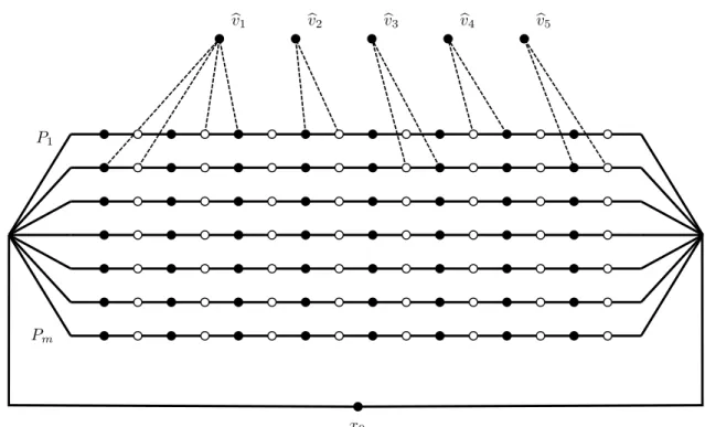
We first sketch the main idea of the proof. We give the reduction from an arbitrarySATinstance onn variables and m clauses. The idea is to create a family of n very long paths P₁, P₂, . . . , P_n of even length, corresponding to variables x1, x2, . . . , xn. Assume for now that on each of these