Cloud workload prediction based on workflow execution time discrepancies

Cloud workload prediction based on workflow execution time discrepancies

Gabor Kecskemeti^{1 •}Zsolt Nemeth^2• Attila Kertesz^3• Rajiv Ranjan⁴

Received: 27 October 2017 / Revised: 1 February 2018 / Accepted: 23 March 2018 / Published online: 16 October 2018 ÓThe Author(s) 2018

Abstract

Infrastructure as a service clouds hide the complexity of maintaining the physical infrastructure with a slight disadvantage:

they also hide their internal working details. Should users need knowledge about these details e.g., to increase the reliability or performance of their applications, they would need solutions to detect behavioural changes in the underlying system.

Existing runtime solutions for such purposes offer limited capabilities as they are mostly restricted to revealing weekly or yearly behavioural periodicity in the infrastructure. This article proposes a technique for predicting generic background workload by means of simulations that are capable of providing additional knowledge of the underlying private cloud systems in order to support activities like cloud orchestration or workflow enactment. Our technique uses long-running scientific workflows and their behaviour discrepancies and tries to replicate these in a simulated cloud with known (trace- based) workloads. We argue that the better we can mimic the current discrepancies the better we can tell expected workloads in the near future on the real life cloud. We evaluated the proposed prediction approach with a biochemical application on both real and simulated cloud infrastructures. The proposed algorithm has shown to produce significantly ( 20%) better workload predictions for the future of simulated clouds than random workload selection.

Keywords Workload predictionCloud computingSimulationScientific workflow

1 Introduction

Infrastructure as a Service (IaaS) clouds became the foundations of compute/data intensive applications [2].

They provide computational and storage resources in an on demand manner. The key mechanism of IaaS is virtuali- sation that abstracts resource access mechanisms with the help of Virtual Machines (VM) allowing their users to securely share physical resources. While IaaS clouds offer some means to control a virtual ensemble of resources (so called virtual infrastructures), they inherently provide no means for precise insight into the state, load, performance of their resources, thus the physical layer is completely hidden. Due to the multi-tenant environment of clouds, application performance may be significantly affected by other, (from the point of view of a particular user) unknown and invisible processes, the so-called background work- load. Albeit Service Level Agreements (SLA) define the expected specifics and various Quality of Service (QoS) methods are aimed at their fulfilment, yet they can provide

& Gabor Kecskemeti

g.kecskemeti@ljmu.ac.uk Zsolt Nemeth

nemeth.zsolt@sztaki.mta.hu Attila Kertesz

keratt@inf.u-szeged.hu Rajiv Ranjan

raj.ranjan@ncl.ac.uk

1 Department of Computer Science, Liverpool John Moores University, Liverpool L3 3AF, UK

2 Laboratory of Parallel and Distributed Systems, MTA SZTAKI, Budapest 1111, Hungary

3 Software Engineering Department, University of Szeged, Szeged 6720, Hungary

4 School of Computing, Newcastle University, Newcastle upon Tyne NE4 5TG, UK https://doi.org/10.1007/s10586-018-2849-9(0123456789().,-volV)(0123456789().,-volV)

a very broad range of performance characteristics only [13].

This article studies performance issues related to the—

unknown—background load and proposes a methodology for its estimation. We envision a scenario where modifi- cations in the virtual infrastructure are necessary at runtime and to make the right decisions and take actions the background load cannot be omitted. As follows, we made two assumptions: (i) the application runs long enough so that the time taken by a potential virtual infrastructure re- arrangement is negligible and (ii) the application is exe- cuted repeatedly over a period of time. Both these assumptions are valid for a considerably large class of cloud based applications. Scientific workflows are espe- cially good candidates for exemplifying this class as they are executed in numerous instances by large communities over various resources [20]. During execution, jobs of a workflow are mapped onto various resources e.g., a parallel computer, a cluster, a grid, a virtual infrastructure on a cloud, etc. Efficient execution of workflows requires a precise scheduling of tasks and resources which further- more, requires both timely information on the resources and the ability to control them. Thus we have chosen sci- entific workflows as a subject and evaluation example of our method.

The recurring nature of workflows enables the extraction of performance data and also successive adaptation, refinement and optimisation leading to dynamic workflow enactment. The main motivation for our work stems from the assumption that by extracting information from past workflow executions, one couldidentify current and pre- dict future background workloads of the resources allo- cated for the workflow. The result of this prediction subsequently enables to steer current and future cloud usage accordingly, including the option of resource re-ar- rangement if indicated. The idea is centred around a set of past load patterns (a database of historic traces). When a workflow is being enacted, some of its jobs have already been executed and some others are waiting for execution.

Our workload prediction aims at finding historic traces, that likely resemble the background of workload behind the currently running workflow. Hence, future tasks (even those that are completely independent from the workflow that was used for the prediction) are enacted taking into consideration the recent background load estimations.

The main contributions of this article are: (i) the concept of a private-cloud level load prediction method based on the combination of historic traces, aimed at improving execution quality (ii) an algorithm for realising the load prediction at runtime so that performance constraints are observed, and (iii) an evaluation of this approach using a biochemical application with simulations using historic traces from a widely used archive.

The remainder of this article is as follows: Sect. 2pre- sents related work, then Sect. 3 introduces the basic ter- minology and assumptions of our research. Section4 introduces our new algorithm. Section5 presents its eval- uation with a biochemical application. Finally, the contri- butions are summarised in Sect.6.

2 Related work

In this article, we examine past traces of certain workflows, and predict the expected background load of the clouds behind current workflow instances. Our technique fits in the analyse phase of autonomous control loops (like monitor-analyse-plan-execute [8]). Similarly, Maurer et al.

[18] investigated adaptive resource configuration from a SLA/QoS point of view using such a loop. In their work, actions to fine tune virtual machine (VM) performance are categorised hierarchically as so called escalation levels.

Generally, our work addresses a similar problem (our scope is on the background workload level instead of infras- tructure and resource management) with a different grained action set for the plan-execute steps of the autonomous loop.

Concerning workload modelling, Khan et al. [12] used data traces obtained from a data centre to characterise and predict workload on VMs. Their goal was to explore cross- VM workload correlations, and predict workload changes due to dependencies among applications running in dif- ferent VMs—while we approach the load prediction from the workflow enactment point of view.

Li et al. [14] developed CloudProphet to predict legacy application performance in clouds. This tool is able to trace the workload of an application running locally, and to replay the same workload in the cloud for further investi- gations and prediction. In contrast, our work presents a technique to identify load characteristics independent from the workflow ran on cloud resources.

Fard et al. [7] also identified performance uncertainties of multi-tenant virtual machine instances over time in Cloud environments. They proposed a model called R-MOHEFT that considered uncertainty intervals for workflow activity processing times. They developed a three-objective (i.e., makespan, monetary cost, and robustness) optimisation for Cloud scheduling in a com- mercial setting. In contrast to this approach our goal is to identify patterns in earlier workloads to overcome the uncertainty, and apply simulations to predict future back- ground load of the infrastructure.

Calheiros et al. [5] offers cloud workload prediction based on autoregressive integrated moving average. They argue that proactive dynamic provisioning of resources could achieve good quality of service. Their model’s

accuracy is evaluated by predicting future workloads of real request traces to web servers. Additionally, Magalhaes et al. [15] developed a workload model for the CloudSim simulator using generalised extreme value/lambda distri- butions. This model captures user behavioural patterns and supports the simulation of resource utilisation in clouds.

They argue that user behaviour must be considered in workload modelling to reflect realistic conditions. Our approach share this view: we apply a runtime behaviour analysis to find a workflow enactment plan that best mat- ches the infrastructure load including user activities.

Caron et al. [6] used workload prediction based on identifying similar past occurrences of the current short- term workload history for efficient resource scaling. This approach is the closest to ours (albeit, we have a different focus support for on-line decision making in scientific workflow enactors etc.), as it uses real-world traces from clouds and grids. They examine historic data to identify similar usage patterns to a current window of records, and their algorithm predicts the system usage by extrapolating beyond the identified patterns. In contrast, our work’s specific focus on scientific workflows allows the analysis and prediction of recently observed execution time dis- crepancies, by introducing simulations to the prediction and validation phases.

Pietri et al. [19] designed a prediction model for the execution time of scientific workflows in clouds. They map the structure of a workflow to a model based on data dependencies between its nodes to calculate an estimated makespan. Though the goal of this paper, i.e. to determine the amount of resources to be provisioned for better workflow execution based on the proposed prediction method is the same in our article, we rely on the runtime workflow behaviour instead of its structure. This means we aim to predict the background load instead of the execution time of a workflow.

Besides these approaches, Mao et al. proposed a com- bined algorithm in [16] for prediction, arguing that a single prediction algorithm is not able to estimate workloads in complex cloud computing environments. Therefore they proposed a self-adaptive prediction algorithm combining linear regression and neural networks to predict workloads in clouds. They evaluated their approach on public cloud server workloads, and the accuracy of their results on workload predictions are better compared to purely neural network or linear regression-based approaches.

Brito and Arau´jo [3] proposed a solution for estimating infrastructure needs of MapReduce applications. Their suggested model is able to estimate the size of a required Hadoop cluster for a given timeframe in cloud environ- ments. They also presented a comparative study using similar applications and workloads in two production Hadoop clusters to help researchers to understand the

workload characteristics of Hadoop clusters in production environments. They argued that the increased sharing of physical computing host resources reduces the accuracy of their model. In this paper we exploit these inaccuracies in order to provide insights into the inner working of the utilised shared cloud resources.

Matha´ et al. [17] stated that estimating the makespan of workflows is necessary to calculate the cost of execution, which can be done with the use of Cloud simulators. They argued that an ideal simulated environment produces the same output for a workflow schedule, therefore it cannot reproduce real cloud behavior. To address this requirement, they proposed a method to add noise to the simulation in order to equalise the simulated behavior with the real cloud one. They also performed a series of experiments with different workflows and cloud resources to evaluate their approach. Their results showed that the inaccuracy of the mean value of the makespan was significantly reduced compared to executions using the normal distribution. A similar variance based workflow scheduling technique was investigated by Thaman and Singh [21], where they eval- uated dynamic scheduling policies with the help of WorkflowSim. In both cases, the authors added artificial variance for workflow’s tasks. In contrast, we do not only introduce realistic background workload, but expose the matched workload as a characterisation of the used cloud.

3 Background

An enactment plan describes the jobs of a scientific workflow, their schedule to resources, and it is processed by a workflow enactor that does the necessary assignments between jobs and resources. If a workflow enactor is cap- able to handle dynamic environments [4], such as clouds, the resources form a virtual infrastructure (crafted to serve specific jobs). In our vision, the enactment plan also lists the projected execution time of each job in the workflow.

Workflow enactors are expected to base the projected execution time on historic executions to represent their expectations wrt. the job execution speed. This enactment extension allows the workflow enactor to offer background knowledge on the behaviour past runs of the workflow that combined the use of various distinct inputs and resource characteristics. As a result, during the runtime of the workflow, infrastructure provisioning issues could be pin- pointed by observing deviations from the projected exe- cution time in the enactment plan.

The virtual infrastructures created by the enactor are often hosted at IaaS cloud providers that tend to feature multi-tenancy and under provisioning for optimal costs and resource utilisation. These practices, especially under pro- visioning, could potentially hinder the virtual

infrastructure’s performance (and thus the execution times of jobs allocated to them). In accordance with the first phase (monitor) of autonomous control loops, to maintain the quality and to meet the SLAs set out for the virtual infrastructure in the enactment plan, the workflow enactor or a third party service continuously monitors the beha- viour of the applications/services/workflows running on the virtual infrastructure. In case of deviations, actions in the management of the virtual infrastructure should take place, such as adding or removing new computing/storage com- ponents, to minimize fluctuations in the quality of execu- tion (note: these reactive actions are out of scope of this article). We assume sufficiently small, likely private, cloud infrastructures where the workflow instances could expe- rience significant enough portion of the whole infrastruc- ture allowing the exploitation of the identified deviations for prediction purposes.

We represent workflowsW2 W(whereWis the set of all possible abstract workflows) as an ordered set of jobs:

W¼ fj1. . .jNg, where the total number of jobs in the

workflow isN2N. The job order is set by their projected completion time on the virtual infrastructure whereas the job inter-relations (dependencies) are kept in the domain of the workflow enactors. The projected execution time of the a job (jx2W) isrexðjxÞ– whererex:W!R^þ. We expect the enactor to calculate the projected execution times based on its background knowledge about thousands of past runs.

We refer to a workflow instance (i.e., a particular exe- cution of the abstract workflow W) with the touple:

½W;t:W T—i.e., the workflow and the start time (tand T depicts the set of all time instances) of its first job½j1;t.

Hence, all instances of jx2W are also identified as

½jx;t:j_x2 ½W;T . Once the workflow started, the enac- tor’s monitoring facilities will collect the observed exe- cution times for each job instance. We denote these as:

robðjx;tÞ—whererob:W T !R^þ.

Using the acquired data from the enactors and its monitoring facilities, we define the error function of (partial) workflow execution time to determine the devia- tion in execution time of a particular workflow suffered compared to the projected times in the enactment plan.

Such function is partial if the evaluated workflow instance is split into two parts: jobsj₁; :::j_kalready executed whereas j_kþ1; :::jN are not yet complete or waiting for execution;

when k¼N the workflow instance is done and the error function determines its final execution time error. So in general, the error function of workflow execution time is defined as:E:W T N!R^þ.

We require that error functions assign higher error val- ues for workflow instances that deviate more from the projected runtime behaviour set in their enactment plan.

These functions should also penalise both positive and

negative execution time differences ensuring that the exe- cution strictly follows the plan. The penalties applied here will allow us to detect if the background workload reduces/

improves the performance of the workflow instance com- pared to the enactor’s expectations. These penalties are exploited by the later discussed workload prediction tech- nique: it can tell if a particular workload estimate is not sufficiently close to its actual real life counterpart. For example, when the execution times show improvements—

negative differences—under a particular workload esti- mates, then the prediction technique knows it still has a chance to improve its estimate (allowing other, not nec- essarily long running, applications to better target the expected background workload on the cloud of the workflow).

The penalties are also important from the point of view of the workflow enactor. The enactment plan likely con- tains projected values resulted from several conflicting service level requirements (regarding the quality of the execution). These projected values are carefully selected by the enactor to meet the needs of the workflow’s user and follow the capabilities of the used cloud resources. Thus, error functions should indicate if the fulfilment of the projected values set by the enactor are at risk (i.e., they should penalize with higher error values even if the observed execution times turned out to be better than originally planned). For example, if we have jobsjxandjy

wherejyis dependent on the output ofjxand several other factors, these factors could make it impossible forj_y to be ready for execution by a the time a better performing jx

completes. Thus, the enactor could make a plan relaxed for jxand explicitly ask for its longer job execution time. If the job is executed more rapidly in spite of this request, the penalty of the error function would show there were some unexpected circumstances which made the job faster.

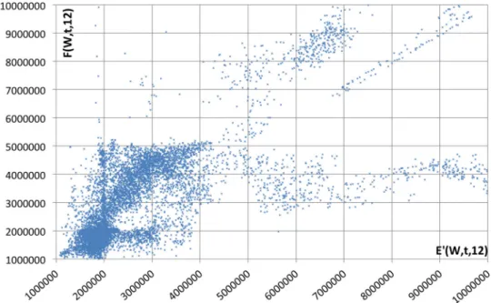
The deviation from the projected execution times (as indicated by the error function) could either be caused by (i) an unforeseen reaction to a specific input, or by (ii) the background load behind the virtual infrastructure of the workflow. In case (i), the input set causes the observed execution times to deviate from the projected ones. Such deviations are rare, because job execution times on a dedicated infrastructure (i.e., only dependent on input values) usually follow a Pareto distribution [1]. Thus, job execution times mostly have small variances, but there could be jobs running several orders of magnitude slower than usual. Figure1 exemplifies this behaviour with a sample of over 20 k jobs ran for various cloud simulation workflows. As it can be observed on the example figure, the long execution times in the slowest 5 % of the jobs cannot be mistaken for perturbations caused by background load.

On the other hand (ii), under-provisioning in IaaS clouds can cause significant background load variation yielding observable (but minor) perturbations in job execution times. In this article, we focus on case (ii) only, therefore we must filter observed execution times whether they belong to case (i) or (ii). Consequently, when observing a significant increase in job execution time (i.e., enactor’s predicted execution time is a magnitude smaller than what was actually observed), we assume that the particular job belongs to case (i) and we do not apply our technique.

However, when we only observe minor deviations from our execution time expectations, we assume that they are of case (ii), caused by the under-provisioned cloud behind the virtual infrastructure executing the observed jobs.

Below, we present a few workflow execution time error functions that match the above criteria. Later, if we refer to a particular function from below, we will use one of the subscripted versions of E, otherwise, when the particular function is not relevant, we just use E without subscript.

Although the algorithm and techniques discussed later are independent from the applied E function, these functions are not interchangeable, their error values are not compa- rable at all.

Average distance. This error function calculates the average time discrepancy of the firstkjobs.

ESQDðW;t;kÞ:¼

ffiffiffiffiffiffiffiffiffiffiffiffiffiffiffiffiffiffiffiffiffiffiffiffiffiffiffiffiffiffiffiffiffiffiffiffiffiffiffiffiffiffiffiffiffiffiffiffiffiffiffiffiffiffiffi P

1ikðrexðjiÞ robðji;tÞÞ² k

s

ð1Þ

Mean absolute percentage error.Here the relative error of the observed runtime is calculated for each job, then it is averaged for allkjobs:

EMAPEðW;t;kÞ:¼100 k

X

1ik

jrexðjiÞ robðji;tÞj

r_exðjiÞ ð2Þ

Time adjusted distance.The function adjusts the execu- tion time discrepancies calculated in ESQD so that the jobs started closer (in time) tojk will have more weight in the final error value.

E_TAdjSQDðW;t;kÞ:¼

ffiffiffiffiffiffiffiffiffiffiffiffiffiffiffiffiffiffiffiffiffiffiffiffiffiffiffiffiffiffiffiffiffiffiffiffiffiffiffiffiffiffiffiffiffiffiffiffiffiffiffiffiffiffiffiffiffiffiffi P

1ik i

kðrexðjiÞ robðji;tÞÞ² P

1ik i k

s

ð3Þ

4 Workflow enactment and simultaneous prediction

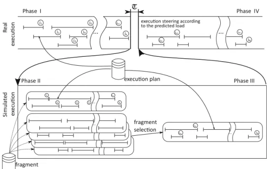
When jobjkis completed during the execution (phase I in Fig.2), a deviation analysis is performed using one of the error functions of Eqs.1–3 to compare the actual job execution times to the ones in the enactment plan. Signif- icant deviations—EðW;t;kÞ[E, where E is predefined by the workflow developer—initiate the background workload prediction phase that corresponds to the second, Analysis phase of autonomous control loops. This phase is omitted, if the workflow enactor estimates the remaining workflow execution time is smaller than required for background workload prediction. The maximum time spent on workload prediction is limited by a predefinedT, rep- resented as a gap in the execution in Fig. 2. Thus, workload prediction is not performed ifPN

i¼kþ1r_exðjiÞ\T.

4.1 Background workload prediction

In essence, we simulate the workflow execution on a given cloud infrastructure while adding known workloads as background load (phase II in Fig.2). The workflow is sim- ulated according to the enactment plan specified runtime properties, like job start time, completion time, and times for creating virtual machines. We expect the simulated work- flow to match its real-world counterpart (in terms of runtime properties), when the added background load closely esti- mates the real-world load. We use Eqs. 1–3to find the known workload closest to the observed one (note: only one function should be used during the whole prediction procedure). Next, we present the details of Algorithm 1 that implements this background workload matching mechanism.

4.1.1 Base definitions

Before diving into the details, we provide a few important definitions: trace fragment—used to provide a particular background workload –, past error—determines the pre- viously collected execution time error values regarding the completed jobs j1; :::jk—finally, future error—defines the previously collected execution error evaluations of the jobs j_kþ1; :::j_N that have not yet run in the current workflow instance (i.e., what was the level of error in the ‘‘future’’

that after a particular past error value was observed).

Atrace fragment is a list of activities characterised by such runtime properties (e.g., start time, duration, Fig. 1 Example distribution of job execution times in a scientific

workflow (where 95% of the execution time is spent on 5 % of the jobs)

performance, etc.) that are usable in simulators, their col- lection is denoted as fragment database in Fig.2. Each fragment represents realistic workloads i.e., real-world system behaviour. Fragments are expected to last for the duration of the complete simulation of the workflow with all its jobs. The fragment duration is independent from the actual real life situation modelled—which stems from the actual½jk;tjob which triggered the prediction. In a worst case, fragments should last for the completely serial exe- cution of the workflow:P

i¼1...krobðjiÞ þP

i¼kþ1...NrexðjiÞ.

Thus fragment durations vary from workflow-to-workflow.

Apart from their duration, fragments are also characterised and identified by their starting timestamp, i.e., the time instance their first activity was logged, denoted as t2T (whereT T); later we will refer to particular fragments by their identifying starting timestamp (despite these fragments often-times contain thousands of activities). As a result, when the algorithm receives an identifying times- tamp, it queries the trace database for all the activities that follow the first activity for the whole duration of the fragment. Note, that our algorithm uses the relative posi- tion of these timestamps. Therefore, when storing historic traces as fragments, they are stored so that their timestamps are consistent and continuous, this requires some dis- placement of their starting positions. This guarantees that we can vary the fragment boundaries (according to the workflow level fragment duration requirements) at will.

Arbitrary selection of fragment boundaries would result in millions of trace fragments. If we would simulate with every possible fragment, the analysis of a single situation would take days. However, as with any prediction, the longer time it takes the less valuable its results become (as

the predicted future could turn past by then). Predictions typically are only allowed to run for a few minutes as a maximum, thus the entire simulation phase must not hinder the real execution for more than T. In the following, we survey the steps that are necessary to meet this requirement i.e., reducing the analysis time from days to T. The frag- ment database needs to be pre-filtered so only a few fragments (T_filtT) are used in the analysis later on.

Although this is out of scope of the current article, pre- filtering can use approaches like pattern matching, runtime behaviour distance minimisation (e.g., by storing past workflow behaviour—for particular fragments—and by comparing to the current run to find a likely start timestamp), or even random selection. Filtering must take limited and almost negligible time. In our experiments, we assumed it belowT=1000 (allowing most of the time to be dedicated to the simulation based analysis of the situation). As a result of filtering, the filtered fragment count must be reduced so that the time needed for subsequent simulations does not exceed the maximum time for predictions: jTfiltj\T=tsimðWÞ, wheretsimis the mean execution time ofWin the simulated cloud. Our only expectation that the pre-filtering happens only in memory and thus the fragment database is left intact.

As a result, when we run the algorithm, it only sees a portion of the fragment database. On the other hand, future runs of the algorithm might get a different portion from the database depending on the future runtime situation.

Finally, we dive into the error definitions. Alongside fragments, several error values are stored in the fragment database, but unlike fragments, which are independent from workflows, these error values are stored in relation to a particular workflow and its past instances. Later, just like

...

...

...

Real execuonSimulated execuon

jk+1

j₁ j₂

j₃ j₄

j₅ j_k-1

j_k

j1

j2 j3 j4

jk-1

jk

...

...

...

...

fragment databse

jk+2

jN

execuon plan T

fragment selecon

V I e s a h P I

e s a h P

Phase III Phase II

execuon steering according to the predicted load

jk+1 jk+2

jN jN-1

...

Fig. 2 Phases of our workload prediction in relation to the workflow being ran

projected execution times, these stored error values are also used to steer the algorithm. First, in terms ofpast errors, we store the values from our previous partial execution time error functions, Eqs.1–3. Past errors are stored for every possiblekvalue for the particular workflow instance.

We calculate future errors similarly to past errors. Our calculation uses the part of the workflow containing the jobs after jk:W^FðW;kÞ:¼ f8ji2W :i[k^iNg, whereW^F 2 W. Thus, the future error function determines how a particular, previously executed workflow instance continued after a specific past error value:

FðW;t;kÞ:¼EðW^FðW;kÞ;t;NkÞ: ð4Þ This function allows the evaluation and storage of the final workflow execution time error for those parts of the past workflow instances, which have not been executed in the current workflow execution.

4.1.2 Overview of the algorithm

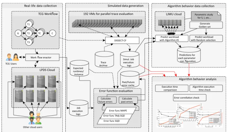
Algorithm 1Fitting based prediction

Require: T^{f ilt}⊂T – the filtered trace fragment set Require: S∈R⁺– the primary search window size Require: Π∈R⁺– the precision of the trace match Require: I∈N– the maximum iteration count

Require: P ∈R⁺ – max evaluations for searching in func- tionφ(x)

Require: [W, t^curr] – the current workflow instance Require: R^ex :={r^ex(jⁱ) :{jⁱ∈W}} – the model execu-

tion times

Require: Rob :={rob(tcurr, ji) :{ji∈W∧i≤k}} – the observed execution times

Ensure: ttargetis around the approximated workload 1: tinit←t∈Tf ilt

2: Tlist← ∅ 3: repeat

4: I←(t^init−S/2, t^init+S/2) 5: R∈2^I\{∅}– arbitrary choice 6: for allt∈Rdo

7: for alljⁱ∈W:i < kdo 8: rex (jⁱ)←r^ob(t^curr, jⁱ) 9: rob (jⁱ, t)←sim(W, R^ex, i, t) 10: end for

11: end for

12: T^red∈2^T\Tlist :|T^red|=P 13: T^min← {t∈T|φ(t) = min

x∈{T_red}φ(x)} 14: t^min←minT^min

15: Tlist←Tlist∪ {t^min}

16: t^target(|Tlist|)← {tl∈T:F(W, tl, k)−E(W, tl, k) = min

tmin−S/2<t<tmin+S/2(F(W, t, k)−E(W, t, k))} 17: tinit ← tx ∈ Tf ilt : |tx − ttarget(|Tlist|)| =

mint∈Tf ilt|t−ttarget(|Tlist|)|

18: until (|ttarget(|Tlist|)− ttarget(|Tlist| −1)| > Π)∧ (|Tlist|< I)

19: return ttareget(|Tlist|)

Algorithm 1 (also depicted functionally in Fig.3 and structurally as phases II–III in Fig. 2) aims at finding a timestamp so that the future estimated error is minimal, while past error prediction for this timestamp is the closest to the actual past error (i.e., the estimated and actual ‘‘past errors are aligned’’). The algorithm is based on the assumption that if past workloads are similar (similarity measured by their error functions) then future workloads would be similar, too.

In detail, line 1 picks randomly one of the fragments identified by the timestamp in the filtered setTfiltand stores int_init. This will be the assumed initial location of the frag- ment that best approximates the background load. Later, in line 17, thistinitwill be kept updated so it gives a fragment that better approximates the background load. Theprimary search window—Rof line 5 also shown between the dashed lines of the lower chart in Fig.3represents a set of times- tamps within aS / 2 radius from the assumed start of the fragment specified by tinit. The algorithm uses set Tlist to store timestamps for the approximate trace fragments as well as to count the iterations (used after line 15).

A simulator is used to calculate observed execution times r⁰_ob for the jobs in the simulated infrastructure (see line 9).

This is expressed withsimðW;Rex;i;tÞthus, each simulation receives the workflow to be simulated, the set of execution time expectations (Rex) that specify the original enactment plan, the identifier of the job (1iN) we are interested in and the timestamp of the trace fragment (t2T) to be used in

Iteration N Iteration a

eration N n N Iteration N N+1

x x x x

xx

x x

x

S S

t

t

E'(W ,t,k)

t

x

a te

x

t

E(W ,t,k)

t t

t

F(W ,t,k)

t

Iteration N on N

2 ation N a S

on N

x

N tera

tion N at Itera

tiont It

erate It t

x x

lines 1,17 ->

lines 17,18 ->

line 12 ->

lines 13,14 ->

line 9 ->

line 4 ->

<- line 16

<- line 17

S/2 S/2

Fig. 3 Visual representation of the algorithm

the simulation as background load to the workflow, respec- tively. With these parameters the simulator is expected to run all the activities in the trace fragment identified bytin par- allel to a simulated workflow instance. Note: the simulation is done only once for the complete workflow for a given infrastructure and a given fragment, later this function sim- ply looks up the past simulatedr_ob⁰ values.

Next, we use one of the error functions of the workflow execution time as defined in Eqs.1–3. As we have simu- lated results, we substitute the observed/expected execution time values in the calculation with their simulated coun- terparts. In the simulation, the expected execution timesr⁰_ex are set as the real observed execution timesrob(see line 8).

To denote this change in the inputs to the error function, we use the notation ofE⁰ðW;t;kÞ—error of simulated execu- tion time. This function shows how the simulated workload differs from the observed one. The evaluation of the E⁰ function is depicted withmarks at the bottom chart of Fig.3.

Afterwards, lines 12–14 search through the past error values for each timestamp (using the same error function as we used for the evaluation ofE⁰). With the help of function /:T !R:

/ðxÞ:¼X

t2R

E⁰ðW;t;kÞ EðW;xþtt_initþS=2;kÞ

ð5Þ This function offers the difference between the simulated and real past error functions (Fig.3represents this with red projection lines between the chart ofEand themarks of E⁰). The algorithm uses the/ðxÞfunction to find the best alignment between the simulated and real past error func- tions: we settminas the time instance inRwith the smallest difference between the two error functions. The alignment is searched over an arbitrary subset of the timestamps:

T_red—thesecondary search window. The algorithm selects aTred with a cardinality ofPin order to limit the time to search for tmin. The arbitrary selection of Tred is used to properly represent the complete timestamp set ofT.

After finding tmin, we have a timestamp from the frag- ment database, for which the behaviour of the future error function is in question, this corresponds to the fragment selection in Fig.2. Line 16 finds the timestamp that has the closest past and future error values in the range aroundtmin

within radius S / 2—see also in the top right chart of Fig.3. Note, this operation utilises our assumption that past and future errors are aligned (i.e., a trace fragment with small past error value is more likely to result in similarly small future error value). The timestamp with the future error value closest to the past error is used asttargetfor the current iteration (i.e., our current estimate for the start timestamp of the approximate background load).

Finally, the iteration is repeated until the successive change in ttarget is smaller than the precision P or the iteration count reaches its maximum—I, represented as phase III in Fig.2. Note, I is set so the maximum time spent on workload prediction (T) is not violated. The algorithm then returns with the last iteration’sttarget value to represent the starting timestamp of the predicted trace fragment that most resembles the background load cur- rently experienced on the cloud behind the workflow. This returned value (and the rest of the trace fragment following ttarget) then could be reused by when utilizing the real life version of the simulated cloud. For example, the workflow enactor could use the knowledge of the future expected workload for the planning and execution phases of its autonomous control loop (phase IV in Fig.2). Note, the precise details on the use of the predicted workload is out of the scope of this article.

5 Evaluation with a biochemical workflow

We demonstrate our approach via a biochemical workflow that generates conformers by unconstrained molecular dynamics at high temperature to overcome conformational bias then finishes each conformer by simulated annealing and/or energy minimisation to obtain reliable structures. It uses the TINKER library [11] for molecular modelling for QSAR studies for drug development.

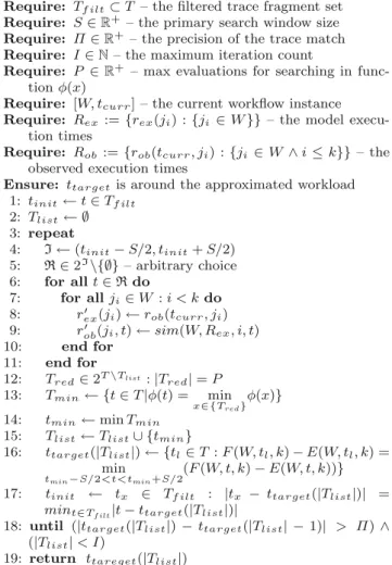
Our evaluation approach is summarized in Fig. 4. It is composed of three main phases: (i) data collection from a real life environment, (ii) modelling the TCG workflow and simulating its behaviour under various background loads, and (iii) evaluating the algorithm based on the collected real life and simulated data.

5.1 The tinker workflow on the LPDS cloud

The TINKER Conformer Generator (TCG) workflow [11]

consists of 6 steps (see the top left corner of Fig.4): (i)G:

generating 50,000 input molecule conformers (taking around 12 h, compressed into 20 zip files by grouping 2500 conformers); (ii)T1: minimising the initial conformational states generated at high temperature; (iii)T2: performing a short low temperature dynamics with the high temperature conformations to simulate a low temperature thermody- namic ensemble, and minimising the above low tempera- ture states; (iv)T3: cooling the high temperature states by simulated annealing, and minimising the annealed states;

(v) TC: collecting parameter study results; (vi) C: re- compressing results to a single file. The sequential execu- tion of the workflow on a single core 2 GHz CPU takes around 160 h.

Note that the parallel section of the workflow could be partitioned arbitrarily: by changing howGsplits the input molecule conformers. For example, any options could be chosen from the extreme case of each molecule becoming an input for a separateT1/2/3/Crun, to the other extreme of having a single zip file produced and processed in a singleT1/2/3/C. Also, if a larger infrastructure is available, more input molecule conformers could be considered in a single run (this would result in a longer execution time for G).

In the period of over half a year, the workflow was ran several times on the cloud of the Laboratory of Parallel and Distributed Systems—LPDS cloud—, which ran OpenNe- bula 4.10 and consisted of 216 cores, 604 GBs of memory and 70 TBs of storage at the time of the experiments. We used a workflow enactor without autonomous control mechanisms. We have collected the job execution times for all jobs in the workflow, as well as the time instance when the workflow was started. We have calculated the expected job execution times—r_exðjiÞ—as an average of the execu- tion times observed. This average was calculated from over 500 runs for each step of the TCG workflow. To enable a more detailed analysis of the workflow executions, we have generated larger input sets allowing us to repeatedly exe- cute the parallel section with 20 virtual machines (in our implemented workflow, the 20 machine parallel section was executed 15 times before concluding with the final re-

compression phase—C). This allowed us to populate our initial past and future error values in the cache (i.e., we have calculated how particular workflow instances behaved when expected job execution times are set to be the aver- age of all). Not only the error cache was populated though, the individual robðji;tÞ values were also stored in our database (in total, the collected data was about 320 MBs).

These data stores are shown in Fig.4 as a per instance expected runtimes database,job execution logs) and Past/

Future error cache. The stored values acted as the foun- dation for the simulation in the next phase of our evaluation.

5.2 Modelling and simulating the workflow

This section provides an overview on how the TCG workflow was executed in a simulator. Our choice for the simulator was the open source DISSECT-CF.¹ We have chosen it, because it is well suited for simulating resource bottlenecks in clouds, it has shown promising performance gains over more popular simulators (e.g., CloudSim, Sim- Grid) and its design and development was prior work of the authors [10]. The section also details the captured proper- ties of the TCG workflow, which we collected in previous phase of the evaluation. Then, as a final preparatory step

Real -life data collection

LPDS Cloud

Other cloud users TCG Users

TCG Work ow

T1

T2

T3 TC

G C

Work ow enactor

Simulated data generation

Job execuon

logs Expected runmes/

instance

Error funcon evaluaon

Calculate past errors Calculate

future errors

Error func SQD Error func TAdj-SQD

Error func MAPE Past/Future error cache DISSECT-CF

Trace Archive

Simul. Job execuon logs 192 VMs for parallel trace evaluaon

Algorithm behavior data collecon

Generate Golden set

Predict workload with Algorithm #1

Predict workload with Random selecon

Predicons for each parameter con guraon

LJMU cloud Parametric study for S, I, etc...

Algorithm behavior analysis

Execuon me comparision

Error correllaon check Algorithm execuon

me check

Fig. 4 Our detailed evaluation approach

1 https://github.com/kecskemeti/dissect-cf.

for our evaluation, we present the technique we used to add arbitrary background load to the simulated cloud that is used by the enactor to simulate the workflow’s run.

5.2.1 The model of the workflow’s execution

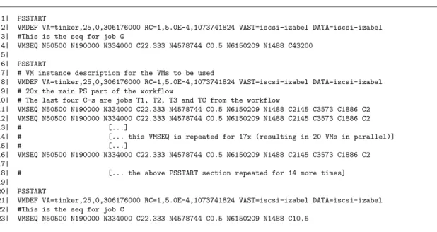
The execution of the TCG workflow was simulated according to the description presented in Fig.5. The description is split into three main sections, each starting with aPSSTART tag (see lines 1, 6 and 20, which corre- spond to the three main sections G–[T1/T2/T3–TC]–C of the TCG workflow shown in the top left corner of Fig.4).

This tag is used as a delimiter of parallel sections of the workflow, thus everything that reside in between two PSSTARTlines should be simulated as if they were exe- cuted in parallel. Before the actual execution though, every PSSTARTdelimited section contains the definition of the kind of VM that should be utilized during the entire parallel section. The properties of these VMs are defined by the VMDEFentry (e.g., see lines 2 or 8) followingPSSTART lines. Note, the definition of a VM is dependent on the simulator used, so below we list the defining details specific to DISSECT-CF:

The virtual machine imageused as the VM’s disk. This is denoted with property nameVA. In this property, we specify that the image is to be called ‘‘tinker’’. Next, we ask its boot process to last for 25 seconds. Afterwards, we specify the VM image to be copied to its hosting PM before starting the VM—0 (i.e., the VM should not run on a remote filesystem). Finally, we set the image’s size as 306 MBs.

The required resourcesto be allocated for the VM on its hosting PM. These resources are depicted behind the property name of RC in the figure. Here we provided details for the number of cores (1), their performance (5.0E-4—this is a relative performance metric com- pared to one of the CPUs in LPDS cloud) and the amount of memory (1 GB) to be associated with the soon to be VMs.

Image originwhere the VM’s disk image is downloaded from before the virtual machine is instantiated. We used the property name ofVASTto tell the simulator the host name of the image repository that originally stores the VM’s image.

Data store is the source/sink of all the data the VM produces during its runtime. This is defined with the property calledDATA. This field helps the simulation to determine the target/source of the network activities later depicted in theVMSEQentries.

The real-life workflow was executed in the LPDS cloud (see the leftmost section of Fig.4). Thus, we needed to model this cloud to match the simulated behaviour of the workflow to its real life counterpart ran in phase one.

Therefore, the storage nameiscsiizabelin the workflow description (e.g., in line 2 of Fig.5) refers to the particular storage used on LPDS cloud, just like the VMI image name tinkerdoes.

Now, we are ready to describe the runtime behaviour of the workflow observed in phase one in a format easier to process by the simulation. This behaviour is denoted with the VMSEQ entries (e.g., see lines 4 or 10) that reside in eachPSSTART delimited parallel section. VMSEQentries are used to tell the simulator a new VM needs to be

1| PSSTART

2| VMDEF VA=tinker,25,0,306176000 RC=1,5.0E-4,1073741824 VAST=iscsi-izabel DATA=iscsi-izabel 3| #This is the seq for job G

4| VMSEQ N50500 N190000 N334000 C22.333 N4578744 C0.5 N6150209 N1488 C43200 5|

6| PSSTART

7| # VM instance description for the VMs to be used

8| VMDEF VA=tinker,25,0,306176000 RC=1,5.0E-4,1073741824 VAST=iscsi-izabel DATA=iscsi-izabel 9| # 20x the main PS part of the workflow

10| # The last four C-s are jobs T1, T2, T3 and TC from the workflow

11| VMSEQ N50500 N190000 N334000 C22.333 N4578744 C0.5 N6150209 N1488 C2145 C3573 C1886 C2 12| VMSEQ N50500 N190000 N334000 C22.333 N4578744 C0.5 N6150209 N1488 C2145 C3573 C1886 C2

] . . . [

#

| 3 1

] ) l e l l a r a p n i s M V 0 2 n i g n i t l u s e r ( x 7 1 r o f d e t a e p e r s i Q E S M V s i h t . . . [

#

| 4 1

] . . . [

#

| 5 1

16| VMSEQ N50500 N190000 N334000 C22.333 N4578744 C0.5 N6150209 N1488 C2145 C3573 C1886 C2 17|

] s e m i t e r o m 4 1 r o f d e t a e p e r n o i t c e s T R A T S S P e v o b a e h t . . . [

#

| 8 1 19|

20| PSSTART

21| VMDEF VA=tinker,25,0,306176000 RC=1,5.0E-4,1073741824 VAST=iscsi-izabel DATA=iscsi-izabel 22| #This is the seq for job C

23| VMSEQ N50500 N190000 N334000 C22.333 N4578744 C0.5 N6150209 N1488 C10.6

Fig. 5 The description of the TCG workflow’s execution for the simulation

instantiated in the parallel section. Each VM requested by the VMSEQentries will use the definition provided in the beginning of the parallel section. All VMs listed in the section are requested from the simulated LPDS cloud right before the workflow’s processing reaches the next PSSTART entry in the description. This guarantees they are requested and executed in parallel (note, despite requesting the VMs simultaneously from the cloud, their level of concurrency observed during the parallel section will depend on the actual load of the simulated LPDS cloud). The processing of the next parallel section, only starts after the termination of all previously created VMs.

In the VMSEQ entries, a VM’s activities before termi- nation. There are two kinds of activities listed: network and compute. Network activities start withNand then followed by the number of bytes to be transferred between theDATA store and the VM (this is the store defined by theVMDEF entry at the beginning of the parallel section). Compute activities, on the other hand, start with the letterCand then they list the number of seconds till the CPUs of the VM are expected to be fully utilised by the activity. VM level activities are executed in the simulated VM in a sequence (i.e., one must complete before the next could start).

For example, line 12 of Fig.5 defines how job execu- tions are performed in a VM. First, we prepare the VM to run the tinker binaries by installing three software pack- ages. This results in three transfers (49 KB, 186 KB and 326 KB files) and a task execution for 22 seconds. Next, we fetch thetinkerpackage (4.4 MBs) and decompress it (in a half a second compute task). Then, we transfer the input files with the 2500 conformers and the required runtime parameters to use them (5.9 MBs and 1.5 KBs). After- wards, we execute the T1, T2, T3 and TC jobs sequentially taking 35, 60, 32 minutes and 2 seconds, respectively.

These values were gathered as the average execution times for the jobs while the real life workflows were running in the LPDS cloud. Finally, this 2 second activity concludes the VMs operations, therefore it is terminated.

The PSSTARTentry in line 6 and the virtual machine executions, defined until line 16, represent a single exe- cution of the parallel section of the TCG workflow.

Because of repetitions, we have omitted the severalVMSEQ entries from the parallel section, as well as several PSSTARTentries representing further parallel sections of conformer analysis. On the other hand, the description offered for the simulator did contain all the 14 additional PSSTARTentries which were omitted here for readability purposes.

To conclude, the description in Fig.5 provides details for over 1800 network and computing activities to be done for a single execution of the TCG workflow. If we consider only those activities that are shown in the TCG workflow,

we still have over 1200 computing activities remaining.

These activities result in the creation and then destruction of 302 virtual machines in the simulated cloud. When calculating the error functions, we would need expected execution details for all these activities or VMs. The rest of the article will assume that the workflow enactor provides details about the computing activities directly relevant for the TCG workflow only (i.e., the jobs ofG/Tx/C). Thus our N value was 1202. The partial workflow execution error functions could be evaluated for every job done in the simulated TCG. This, however, is barely offering any more insight than having an error evaluation at the end of each parallel section (i.e., when all VMs in the particular parallel section are complete). As a result, in the rest of the article, when we report kvalues, they are going to represent the amount of parallel sections complete and not how many actual activities were done so far. To transform between activity count and the reportedkvalues one can apply the following formula:

kreal:¼

k¼0 0

k\15 1þ80k

k¼15 1þ80kþ1;

8<

: ð6Þ

where 15 is the number of parallel sections, and 80 is the number of TCG activities per parallel section. Finally, the kreal is the value used in the actual execution time error formulas from Eqs.1–3.

Although, the above description was presented with our TCG workflow, the tags and their attributes of the description were defined with more generic situations in mind. In general, our description could be applied to workflows and applications that have synchronisation barriers at the end of their parallel sections.

5.2.2 Simulating the background load

In order to simulate how the workflow instances of TCG would behave under various workload conditions, we needed a comprehensive workload database. We have evaluated previously published datasets: we looked for workload traces that were collected from scientific com- puting environments (as that is more likely to resemble the workloads behind TCG). We only considered those traces that have been collected over the timespan of more than 6 months (i.e., the length of our experiment with TCG on the LPDS cloud—as detailed in Sect.5.1). We further filtered the candidate traces to only contain those which would not cause significant (i.e., months) overload or idle periods in the simulated LPDS cloud. This essentially left 4 traces (SharcNet, Grid5000, NorduGrid and AuverGrid) from the Grid Workloads Archive (GWA [9]), we will refer to the summary of these traces asT^GWA T. Note, it is irrelevant

that the traces were recorded on grids—for our purposes the user behaviour, i.e., the variety of tasks, their arrival rate and duration are important. Fortunately, these char- acteristics are all independent from the actual type of infrastructure.

Trace fragments were created using GWA as follows:

we started a fragment from every job entry in the trace.

Then we identified the end of the fragment as follows. Each fragment was expected to last at least for the duration of the actual workflow instance. Unfortunately, the simulated LPDS cloud could cause distortions to the job execution durations (e.g., because of the different computing nodes or because of the temporary under/over-provisioning situa- tions compared to the trace’s original collection infras- tructure), making it hard to determine the exact length of a fragment without simulation. Thus, we have created frag- ments that included all jobs within 3 times the expected runtime of the workflow. As a result each of our fragments was within the following time range: ½t;tþ3P

0\i\N

rexðjiÞ. All these fragments were loaded in the trace archiveof Fig.4 (see its middle section titled ‘‘simulated data generation’’). All together, our database have con- tained more than 2 million trace fragments.

With the trace fragments in place, we had every input data ready to evaluate ther_ob⁰ values under various work- load situations (i.e., represented by the fragments). Thus, we have set out to create a large scale parametric study. For this study, we have accumulated as many virtual machines from various cloud infrastructures as many we could afford. In total, we have had 3 cloud infrastructures (SZTAKI cloud,² LPDS cloud, Amazon EC2³) involved which hosted 192 single core virtual machines with 4 GBs of memory and 5 GBs of hard disk storage (and the closest equivalent on EC2). We offered the trace archive to all of them as a network share. Each VM hosted DISSECT-CF v0.9.6 and was acting as a slave node for our parametric study. The master node (not shown in the figure), then instructed the slaves to process one trace at a time as follows⁴:

1. Load a trace fragment as per the request of master.

2. Load the description of LPDS cloud.⁵

3. Load the description of TCG workflow execution (i.e., the one shown in Fig. 5).

4. Start to submit the jobs from the loaded fragment to the simulated LPDS cloud (for each submitted job, our

simulation asks a VM from the cloud which will last until the job completes).

5. Wait until the 50th job—this step ensures the simu- lated infrastructure is not under a transient load.

6. Start to submit the jobs and virtual machines of the workflow execution specified in the previously loaded description (the VMs here were also ran in the simulated LPDS cloud).

7. For each task, record its observed execution time—

r⁰_obðji;tÞ. Note, here t refers to the start time of the simulated workflow.

8. After the completion of the last job and VM pair in the workflow, terminate the simulation.

9. Send the collected job execution times to master.

The simulation of all trace fragments took less than 2 days.

The mean simulation execution time for a fragment run- ning on our cloud’s model is tsimðTCGÞ ¼756 ms. We have stored the details about each simulation in relation to the particular trace fragment in our simulated job execution log database (see Fig.4).

To conclude our simulated data generation phase, we populated ourpast and future error cacheof Fig.4. Later our algorithm used this to represent past workflow beha- viour. We calculated the past and future error values with the help of allr⁰_obwe collected during the simulation phase.

The error values were cached from all 3 error functions we defined in Eqs.1–3 as well as from their future error counterparts from Eq.4. This cached database allowed us to evaluate the algorithm’s assumptions and behaviour in the simulated environment as we discuss it in the next section.

5.3 Evaluation

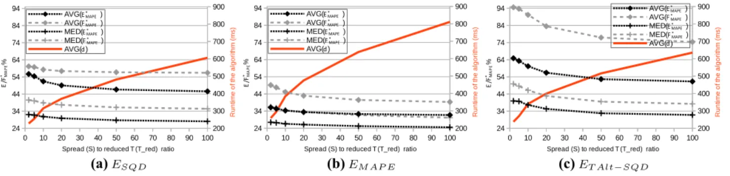
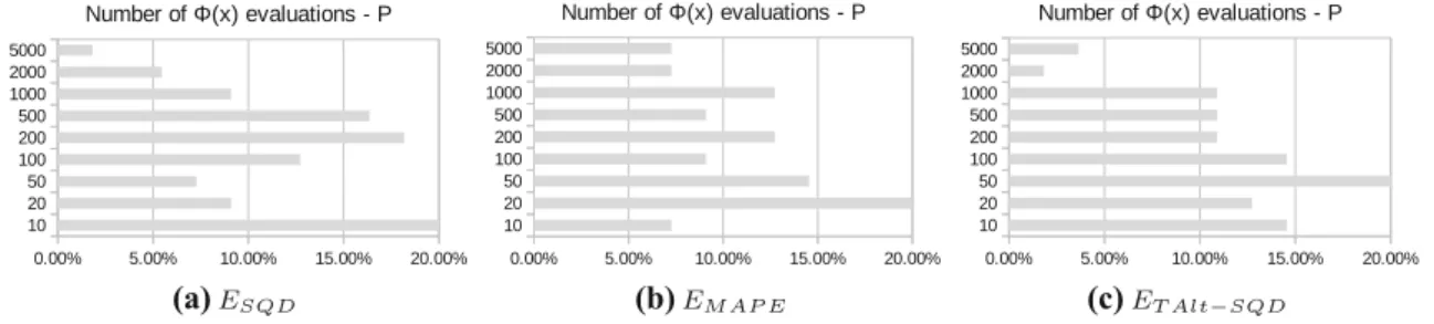
In this section, we evaluate our algorithm using the col- lected data about the simulated and real life TCG workflow instance behaviour. We focused on three areas: (i) analyse our assumption on the relation of past and future errors, (ii) provide a performance evaluation of the algorithm, and (iii) analyse how the various input variables to the algorithm influence its accuracy. These are shown as the last two phases (algorithm behaviour data collection and analysis) in Fig. 4.

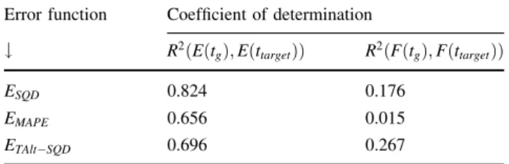
5.3.1 Relation between past and future errors

To investigate our assumption on the relation of past and future error values, we have analysed the collected values in the error cache. In Fig.6, we exemplify how the simu- lated past and future error values (using theESQDfunction) vary within a subset of the past/future error cache (which we collected in the previous phase of our evaluation). Here,

2 http://cloud.sztaki.hu/en.

3 https://aws.amazon.com/ec2.

4 The source code of these steps are published as part of the following project:https://github.com/kecskemeti/dissect-cf-examples/.

5 http://goo.gl/q4xZpe.