COMPUTATIONAL PHYSICS

(1)

COMPUTATIONAL PHYSICS

The Computational Physics Section publishes articles that help students and their instructors learn about the physics and the computational tools used in contemporary research. Most articles will be solicited, but interested authors should email a proposal to the editors of the Section, Jan Tobochnik (jant@kzoo.edu) or Harvey Gould (hgould@clarku.edu). Summarize the physics and the algorithm you wish to include in your submission and how the material would be accessible to advanced undergraduates or beginning graduate students.

Molecular dynamics simulation of a two-dimensional dusty plasma

Istv!anDonk!o,

Faculty of Informatics, E€otv€os Lor!and University, P!azm!any P!eter stny. 1/c, H-1117 Budapest, Hungary

PeterHartmann,and Zolt!anDonk!o^a)

Institute for Solid State Physics and Optics, Wigner Research Centre for Physics, Konkoly-Thege Miklos str.

29-33, H-1121 Budapest, Hungary

(Received 23 July 2019; accepted 20 September 2019)

Two-dimensional dusty plasmas can be realized experimentally and are examples of a classical many body system with a screened Coulomb interaction. After discussing experimental approaches, we present the basics of molecular dynamics simulations of dusty plasmas. A web-based platform is developed that allows users to perform molecular dynamics simulations, visualize the system for selected system parameters, and obtain results for the pair correlation function and the dispersion relation of waves in the system.^V^C2019 American Association of Physics Teachers.

https://doi.org/10.1119/10.0000045

I. INTRODUCTION

Dusty plasmas are systems where millimeter to nanometer sized particles are suspended in a partially ionized gaseous environment consisting of neutral atoms/molecules, electrons, and ions. The initial interest in dusty plasmas origi- nated in the fields of space physics and astrophysics,^1,2 where it was realized that dust particles are naturally present in these environments. More recent developments in gas discharge physics and microelectronics³have led to the recog- nition that dust contamination is naturally present in industrial plasmas due to plasma etching effects as well as dust particle growth through chemical reactions.⁴

A recent experimental breakthrough has been the ability to optically track individual dust grains suspended in discharge plasmas, which provides the possibility of examining the dynamics at the level of individual dust particles.^5–7

In addition to its relevance to numerous topics in plasma physics, including dust charging, dust shielding, ion drag forces, and plasma–surface interactions, dusty plasmas play an important role as analogue systems for investigating complex cross-disciplinary phenomena. For example, experimental studies of nonlinear dynamics and long-range interactions in strongly correlated systems are often challenging because these systems generally require extreme conditions such as very low temperatures (ultracold ion/atom systems) or high densities (high energy density physics). Dusty plasmas allow the formation and study of analogs to such strongly coupled systems, where the potential energy dominates the kinetic energy.⁸ Such studies can be conducted under laboratory conditions at close-to-room temperatures and easily attain- able pressures.⁹Dusty plasma analogues have recently been used to model crystallization dynamics in two dimensions,¹⁰

quantum dot excitation,¹¹nonlinear and shock waves,¹²electrorheological fluids,¹³and viscoelastic materials.¹⁴

Strongly coupled dusty plasmas were initially established in radio frequency excited noble gas discharges using spherical monodisperse solid particles made of glass,¹⁵melamine- formaldehyde,¹⁶ silica,¹⁷ or titanium-dioxide.⁷In these systems, the dust particles acquire a negative electric charge to balance the electron and ion currents flowing to their surfaces, and become confined by the sheath electric fields that form near the electrodes and other surfaces surrounding the gas discharge plasma. In the presence of gravity, thousands of micrometer sized particles can arrange themselves in a quasi-two-dimensional (2D) layer.

In Sec.II, we discuss experimental systems in more detail.

We then discuss the “one component plasma” model and its main parameters in Sec. III. This model has successfully been applied to 2D dusty plasma systems. The basics of the molecular dynamics method, which is one of the main tools for the simulation of dusty plasmas, are presented in Sec.IV, along with illustrative numerical results. SectionVexplains the implementation of this technique using a web-based tool that is freely available and supplements this article.

Suggested problems are given in Sec.VI.

II. EXPERIMENTAL SYSTEMS

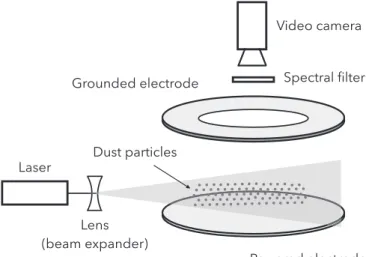
A schematic of an experimental setup is shown in Fig.1.

A low-pressure capacitively coupled radio frequency plasma is established within a vacuum chamber (not shown) between the powered and grounded electrodes. When small dust grains (with a diameter typically in the micrometer range) are introduced into this plasma, they acquire a negative charge¹⁸ of typically 10³–10⁴ elementary charges.

(2)

Because of their high electric charge, the dust particles are levitated above the powered electrode due to the balance of gravity and the electrostatic force that originates from the sheath electric field.¹⁹The horizontal confinement of the dust suspension is ensured by the radial electric field which arises due to the charging of a confining element, for example, a glass tube surrounding the system (not shown in Fig.1).

Images of the particle layer are recorded by a video camera. The observation is aided by illuminating the dust layer with an expanded laser beam with a specific wavelength.

The spectral filter placed in front of the camera transmits this wavelength but blocks most of the radiation from the plasma thereby significantly increasing the contrast. A sequence of recorded images can be used to identify and trace individual particles, providing the position and velocity coordinates of each particle. The length and time scales allow relatively easy observation of the dynamics.

Figure2shows a snapshot of the particles recorded in our experimental setup. Due to the strong interaction between

the particles, most of the particles are located at sites of a triangular lattice. The crystalline ordering is a consequence of the strong electrostatic interaction of the highly charged dust particles which creates a potential energy that is much greater than the kinetic energy of the system. The particles cannot form a perfect lattice due to the boundary conditions in the experimental system and their density slightly varies spatially. Therefore, we observe lattice defects, predomi- nantly dislocations, which appear as bounded pairs of sites with 5 and 7 particles in their nearest neighbor shells, determined by performing a Delaunay triangulation.²⁰The signifi- cance of the different types of lattice defects and their consequences on the topological phase transitions in 2D materials was discovered by Kosterlitz and Thouless.²¹ In dusty plasmas, the static and dynamical properties of these systems have been investigated in detail.^22,23

III. THE ONE-COMPONENT PLASMA MODEL We will discuss the properties of the dust particle system in the plasma environment within the framework of the “one component plasma” model. This model considers only one of the species of the system (the dust particles in our case).

As we have discussed, dust particles acquire a large negative charge in the plasma environment. In the absence of other charged species (the electrons and ions of the surrounding plasma), the dust particles would interact via the r^–1 Coulomb potential. However, the presence of electrons and ions modifies this potential due to an important property of plasmas, Debye screening, which results in deviations of the electron and ion densities from their average density around the dust particles, and leads to the screening of the potential created by the dust particles. It can be shown that, as a consequence, the Coulomb potential is modified by an exponential factor, resulting in a dust particle pair potential of the form²⁴

/ðrÞ ¼Qexpð$r=kDÞ

4pe0r ; (1)

whereQis the charge of the dust particles,kDis the screening (Debye) length, and e0is the permittivity of free space.

The form of the potential in Eq. (1) is known as the Debye–H€uckel or Yukawa potential. If the particles interact via the potential in Eq.(1), the model is often referred to as the “Yukawa one component plasma” model.

The main parameter of the system is the coupling parameter

C¼ Q²

4pe0akBT; (2)

which is the ratio of the Coulomb potential energy at a char- acteristic particle separation aws to the thermal energy kBT (equal to the mean kinetic energy per particle in 2D), where Tis the dust temperature and kBis the Boltzmann constant.

The Wigner-Seitz radius is defined as

aws¼ ðpn0Þ^$1=2; (3)

wheren0is the areal number density of the particles.

The strength of the screening of the Coulomb interaction can be expressed in terms of the dimensionless parameter

j¼aws=kD: (4)

Fig. 1. Schematic of a dusty plasma experiment.

Fig. 2. Experimentally recorded snapshot of a dusty plasma layer for a large value of the coupling parameterC. The configuration is highly ordered with an underlying triangular lattice (identification is aided by the lines in a part of the snapshot). Although most particles have six neighbors, lattice defects result in exceptions that are indicated by circles (five neighbors) and trian- gles (seven neighbors).

(3)

Another important quantity is the plasma frequency x0¼ ffiffiffiffiffiffiffiffiffiffiffiffiffiffiffiffiffiffiffiffiffiffiffiffiffiffiffi

nQ²=2awse0m

p ; (5)

which governs the dynamics of the system. Here,mis the mass of the particles. (Note that the plasma frequency for a 2D system differs from the 3D plasma frequencyx0;3D¼ ffiffiffiffiffiffiffiffiffiffiffiffiffiffiffiffiffiffiffiffiffiffi

n3DQ²=e0m p .)

IV. MOLECULAR DYNAMICS SIMULATIONS Molecular dynamics (MD) simulations produce particle trajectories in phase space by accounting for the interactions between the particles and for the effects of additional forces originating from an external potential (for example, a trap- ping potential) and/or the effect of an embedding environment (for example, friction²⁵). The case that we discuss here is one of the simplest:

(1) We consider a microcanonical (“NVE”) ensemble, where the number of particles, the volume of the system, and the total energy is conserved.

(2) We use point-like charged particles which have only translational degrees of freedom. (Molecules may have additional (for example, rotational) degrees of freedom and their pair interaction may depend on their mutual orientation. The mutual orientation may also become important if the particles have a magnetic moment, which also contributes to inter-particle forces.)

(3) The particles interact via an isotropic pair potential. In experiments, the particle charging is anisotropic due to streaming ions. Neglecting this anisotropy is well justified as long as the particles arrange themselves into a single layer.

(4) The motion the particles is assumed to be frictionless, which is a good approximation for low gas pressures (!1 Pa).

(5) Although particles are confined within a layer by a trap- ping potential in experiments, we idealize the system by assuming that the motion of the particles is restricted to a plane.

(6) We consider a system consisting of a single type of species, although in reality there exists a broad range of multi-component systems.

Our simulations are relevant to the central domain of a large experimental system where the density can be consid- ered to be homogeneous.

The system consists ofNidentical particles confined to a square,H%Hsimulation cell. Given the simplifications we have discussed, the form of the equations of motion for parti- cleiis

m€ri¼X

i6¼j

Fðri;jÞ; (6)

where F (ri,j) is the force between particles i and j, which depends only on their separation ri,j. The summation goes over the particles that make a non-negligible contribution to the total force acting on particlei.

Equation (6)can be solved by using a numerical integra- tion method. We use the velocity-Verlet algorithm²⁶

rðtþDtÞ ¼rðtÞ þvðtÞDtþ1

2aðtÞðDtÞ²; (7) vðtþDtÞ ¼vðtÞ þ1

2½aðtÞ þaðtþDtÞ(Dt: (8)

Because the acceleration appears both attandtþDtin Eq.(8), the computation proceeds as follows:

(1) The particle positions are updated according to Eq.(7), based on the values of the relevant quantities at timet.

(2). From Eq. (8), we compute the intermediate velocity v⁾¼vðtÞ þ ð1=2ÞaðtÞDt.

(3) We calculate the force and aðtþDtÞ based on the updated positions of the particles.

(4) Finally, we calculatevðtþDtÞ ¼v⁾þð1=2ÞaðtþDtÞDt.

These steps are repeated many times to obtain the particle trajectories.

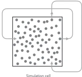
In the simulations, we apply periodic boundary conditions, which eliminate any surfaces so that a particle that leaves the simulation cell is introduced into the cell at the opposite side, without any change of its velocity (see Fig. 3). This condition ensures a homogeneous system and makes it unnecessary to use a confining potential.

The solution of the equations of motion requires the computation of the total force acting on each particle. For a potential that decays sufficiently quickly, for example, the Yukawa potential, we can define a cutoff distancercbeyond which the pair interactions are negligible. As illustrated in Fig.4(a), the force acting on a particle can be obtained by summing over neighboring particles that are situated within a circle of radius rc,centered at the given particle. For particles near the edges of the simulation cell, the circle, which encloses the neighbors, may be partly outside the cell, as shown in Fig. 4(b). In this case, neighbors also have to be searched for in the replicas of the simulation cell (which are copies of the simulation cell shifted by the cell length in one or both directions and which surround the primary simulation cell).

Finding the neighbors efficiently is aided by the “chaining mesh” technique: The simulation cell is divided into sub- cells, and at each time step the particles are assigned to lists corresponding to one of these cells.²⁷The edge length of the sub-cellshis chosen such thath>rc,so that it is sufficient to search for neighbors only in the sub-cell where the given particle resides and in neighboring sub-cells.

Molecular dynamics simulations can be performed at constant temperature, constant pressure, or constant energy. The choice depends on the nature of the effects that are

Fig. 3. Illustration of periodic boundary conditions. Particles that leave the simulation cell are re-introduced at the opposite side, with the same velocity.

(4)

investigated. The results discussed in this section were obtained from simulations where the energy is conserved.

The interactive MD tool that supplements this article, on the other hand, applies an Andersen thermostat²⁶ to ensure that the system equilibrates within a reasonable time at the given values ofCandjvalues set by the user.

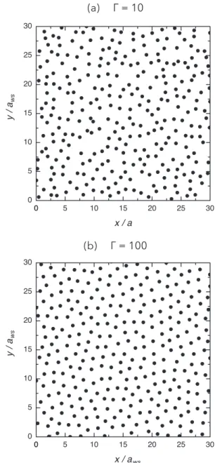
In the following, we illustrate some of the results that can be obtained from the simulations. Figure 5 shows particle snapshots obtained from the simulations for different values ofCandj¼1. ForC¼10, we observe a weak order in the particle positions, which is significantly enhanced when the coupling is increased toC¼100. Ordering is a consequence of the dominance of the interparticle potential energy over the kinetic energy of the particles.

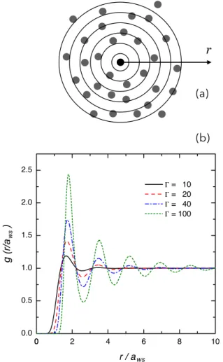
One measure of the degree of regularity of the particle configurations is the pair correlation function g(r). To determineg(r), we count, around a given particle, the number of particles situated within concentric rings as illustrated in Fig. 6(a), and normalize this number by the respective area of these domains and by the average particle density. We then average over all particles. For a random arrangement of the particles (for which the most important example is the ideal gas) the resulting value isgideal(r)¼1.

The pair correlation function g(r) thus expresses the rela- tive density of neighbors around a given particle. By assuming isotropy of the system, which is an inherent char- acteristic of the fluid phase, the pair correlation function

has a single scalar argument, the separation of the particles.

If the system crystallizes, the pair correlation function has a vector argument.

The pair correlation function for the Yukawa fluid at different values ofC is plotted in Fig.6(b). The function g(r) exhibits a “correlation hole” at small separations as a consequence of the repulsion between the particles, which pre- vents them from getting close to each other due to their lack of sufficient kinetic energy. At a distance corresponding to the most probable first neighbor distance, g(r) exhibits a peak, which marks the first coordination shell. This peak is followed by a depleted region and a sequence of other coordination shells, which appear as smaller amplitude peaks in g(r) due to the decay of correlations over longer distances.

The spatial order of fluids extends over a finite distance such that within this distance the fluid “inherits” the structure of the lattice, which is why the peak positions ofg(r) change only slightly with increasingCin Fig.6(b).

Fig. 4. (a) For short-range potentials, it is sufficient to consider neighboring particles within a circle of radiusrcto compute the total force acting on a particle. (b) When periodic boundary conditions are applied, these neighbors might also need to be searched for in replicas of the primary simulation cell.

Fig. 5. Snapshots for (a)C¼10 and (b)C¼100 atj¼1. The spatial coordinates are normalized by the Wigner-Seitz radius. Note the less regu- lar particle arrangement forC¼10 and the more ordered configuration for C¼100.

(5)

The prominent structure of the system for largeCgives rise to quasi-localization of the particles, which means that the particles oscillate in local potential wells of the potential surface created by other particles. For strong coupling⁸(C*1), the change of the potential surface due to the diffusion of the particles is much slower than the time scale of these oscillations. This behavior is the basis of the quasi-localized charge approximation where the dynamical properties are derived from the pair correlation function and the interaction potential.^28,29

An intrinsic property of many-body systems is that they can support collective excitations; for example, gases and liquids support sound waves, which are propagating compressional density perturbations. Waves are not only generated by an external perturbation of the system, but can also be thermally excited, where the motion of the particles of the system gener- ates a (usually low amplitude) density perturbation. The wavelength and the frequency of the waves are determined by the structure of the system and the interparticle interaction.

If the motion of the particles is confined to a plane, two types of waves may develop: longitudinal and transverse waves, as illustrated in Fig. 7(a). (If the motion is not restricted to a plane, but is confined by a parabolic potential that allows particles to move perpendicularly to the plane, there are three different types of waves: Two of them are the same as here; the third, which is also a transverse mode with particle oscillations perpendicular to the plane, has an optic character due to the confining potential.) For longitudinal or

compressional waves, the direction of oscillations is in the same direction as the wave propagation [represented by the wave vector kin Fig. 7(a)]. For transverse or shear waves, the direction of oscillations of the particles is perpendicular to the wave vectork. Transverse waves are unusual in gases and liquids, which cannot sustain shear. The presence of strong correlations enables the existence of shear waves,^23,30 which are strongly damped and consequently have a shorter lifetime compared to compressional waves.

Longitudinal waves propagating in thex–direction can be characterized by the dynamical structure function S(kx,x),

Fig. 6. (Color online) (a) Illustration of the measurement of the pair correlation functiong(r). (b) The pair correlation function of the Yukawa liquid for different values ofCandj¼1.

Fig. 7. (Color online) (a) Longitudinal and transverse waves in a plane;kis the wave vector, which points in the direction of wave propagation, and the arrows indicate the oscillations of the particles. (b) The current fluctuation functionL(k_x,x) forC¼100 andj¼1. The argumentk_xofLimplies that data were collected along thexaxis. The frequency and the wave number are normalized, respectively, by the plasma frequency and the Wigner–Seitz radius. Large values ofL(kx,x) identify waves in the system, and the loci of these values yield the dispersion relationxðkxÞ. Because the system is in the fluid phase, the loci is not a sharp line. The dispersion relation of Yukawa fluids is quasi-acoustic; that is, it is linear for small wave numbers and acquires a square root form at intermediate wave numbers. The slope of xðkxÞat smallkdefines the longitudinal sound speed (Ref.23).

(6)

which gives the spectrum of the density fluctuations. The peaks ofS(kx,x) identify the collective excitations. IfS(kx,x) is computed for a series of wave numbers, the dispersion relationx(kx) of the longitudinal wave can be obtained from the simulations by identifying the x values where S has a peak as a function ofkx. This procedure is easy to carry out for C * 1 for which S exhibits sharp peaks, but is more ambiguous when the peaks of S become broad due to the higher damping or decreasing lifetime of the modes at lower Cvalues.

The computation ofS(kx,x) proceeds by decomposing the particle density in terms of its Fourier components

qðkx;tÞ ¼X^N

j¼1

e^$^ik^x^x^j^ð^t^Þ: (9)

Given a time series ofq(k_x,t), another Fourier transform (in time) is performed to obtain q(kx,x), from which the dynamic structure function is computed as^31,32

Sðkx;xÞ ¼ 1 2pN

1

T0 ½qðkx;xÞq⁾ðkx;xÞ(; (10) whereq⁾ðkx;xÞis the complex conjugate ofq(kx,x) andT0

is the duration of the recording ofq(kx,t).

In addition to the spectrum of density fluctuations, we can compute the spectrum of the current fluctuations, L(kx,x). The longitudinal current fluctuation spectrum is obtained in a similar way as S(kx,x) from Eq. (10) by replacingq(k_x,t) by

kðkx;tÞ ¼X

j

vj;xe^$^ik^x^x^j^ð^t^Þ; (11)

where v_j,x is the x component of the velocity vector of the j-th particle. We note thatS(kx,x) andL(kx,x) are related by Lðkx;xÞ ¼ ðx=kxÞ²Sðkx;xÞ.³³ Because L(kx,x) is usually obtained with better signal to noise ratio in simulations, we computeL(kx,x). (In case of sharp peaks inSðkx;xÞthe positions of the corresponding peaks inL(k_x,x) are very nearly the same, but in general, thex² factor in the above relation may shift the peak positions to some extent.)

For propagation along thexdirection, information can be obtained for waves whose wavelength fits integer times (1;2;…) into the simulation cell, that is, for which the wave numbers obeykx¼nkminðn¼1;2;…Þ, wherekmin ¼2p=H is the minimum wave number. It is conventional to introduce the normalized wave number k#¼kminaws. The normalized minimum wave number, k#min¼2pffiffiffip= ffiffiffiffi

pN

(using Eq. (3) withn0¼N=H²) decreases with increasing density.

Figure7(b)shows an example of the longitudinal current- current fluctuation spectrum,L(k_x,x), forC¼100 andj¼1.

The region with high amplitude indicates that longitudinal waves are present at the given frequency and wave number.

At low wave numbers, kxaws!1, the peaks ofL(kx,x) as a function of x (at a givenkx) are quite sharp, but at higher wave numbers the peaks broaden due to the decrease in the lifetime of collective excitations with increasingkx. At small wave numbers, the dispersion relationxðkxÞis linear, and its slope defines the sound speed. With increasing wave number, the mode frequency starts to deviate from this linear dependence on the wave number, and the mode is said to have a quasi-acoustic character. At even higher values of kx, the

mode frequency saturates and subsequently starts to decrease.

This behavior is reminiscent of the behavior of a mode in a solid, where the frequency is a periodic function of the wave number in the principal directions.

The transverse waves can be analyzed similarly to longitudinal waves by computing the transverse current fluctuation spectrumT(kx,x) from the transverse current

sðkx;tÞ ¼X

j

v_j;ye^$ik^x^x^j^ðtÞ; (12)

by replacingv_j;xby v_j;y in Eq.(11), wherev_j;y?kx. As men- tioned previously, transverse waves are unusual in the liquid phase and can exist in the present system only because of the strong correlations at high C. Because these waves are strongly damped for C*1, their spectrum is quite broad and the mode frequency is more difficult to identify compared to the longitudinal modes.²³ Therefore, we consider only the longitudinal modes in our simulation tool.

V. IMPLEMENTATION

Our MD simulation followsN¼500 particles in a plane.³⁴ Our desire to obtain results and visualize the system in real time limits the value of N. For research purposes, much larger particle numbers are routinely used. The simulation uses a 5%5 chaining mesh, which, with the choice of rc¼H=5, provides sufficient accuracy for the forces acting on the particles even for the smallest value of the screening parameter,j ¼1, for which the decrease in the potential is the slowest.

The particles are initially placed randomly within the square simulation cell with their initial velocity vectors sampled from a Maxwell–Boltzmann distribution. Due to the randomness of the initial configuration, the system needs to be thermalized to reach equilibrium, which is achieved by rescaling the veloci- ties of the particles at each time step to match the desired system temperature. This procedure ensures a fast thermalization of the system, but creates a non-Maxwell–Boltzmann distribution from the initial Maxwell–Boltzmann distribution, and therefore no data are collected during this initial thermalization period.

After turning on data collection at later times, the Andersen thermostat³⁵ is applied to the system: Randomly chosen particles interact with a defined frequency with a heat bath that has a temperature defined by the value ofC. Upon interaction with the heat bath, the particles acquire new velocity vectors that are randomly sampled from a Maxwell–Boltzmann distribution at the desired temperature.

During the simulation, the particle positions are displayed as a function of time, while the actual value of C, the pair correlation function g(r), and the wave behavior are moni- tored in separate panels.

The system parametersCandjcan be adjusted using the graphical interface shown in Fig. 8. Following a change, velocity rescaling is conducted for 1000 time steps, and then accumulation of data forg(r) andL(kx,x) at the new parameter values begins.

The simulation is implemented in JavaScript with the lay- out and interactions defined using HTML and CSS, which runs either in a browser or as a self-contained Electron³⁶ package with the open source Chromium browser bundled with the contents. The rendering of the particles, graphs, and the wave dispersion map use the Web Canvas technology.³⁷

(7)

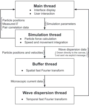
To increase performance, the application is divided into four kinds of threads as illustrated in Fig.9.

• The Main thread handles the front-end, while the three others running in the background handle the bulk of the computation. The results of these worker threads are then sent back to the main thread and displayed on the interface.

• TheSimulation threadprovides the necessary data for the visualization and other calculations.

• The Buffer thread preprocesses the data it receives, thus providing buffer contents for theWave dispersion thread.

There are two instances of this thread running at the same time, one for handling each of the dimensions in the simulation.

• When enough information is accumulated, the Wave dispersion threadexecutes the final steps needed to produce the “heat map” displayed on the interface.

Further details about the implementation can be found in theReadme file, which is attached to the source code of the application, that is available at: https://github.com/Isti115/

dusty-plasma-molecular-dynamics. The online version can be accessed by visiting: https://isti115.github.io/dusty- plasma-molecular-dynamics/. The packaged executables are downloadable from the AJP servers.³⁴

VI. SUGGESTED PROBLEMS

(1) In a hexagonal lattice, the six nearest neighbors are situated at a distance of r1¼b, and the second and third nearest neighbors are atr2 ¼ ffiffiffi

p3

bandr3 ¼2b, respectively, wherebis the lattice constant, which is related to the Wigner-Seitz radius byb¼aws

ffiffiffiffiffiffiffiffiffiffiffiffiffiffiffiffiffi p3

=2p q

ﬃ1:905aws. The first peak ofg(r) occurs at r¼r1forC*1. In the fluid phase, the coordination shells at r2 and r3 are

usually not resolved ing(r). Find the value ofCforj¼ 1, which results in distinct peaks in g(r) for the second and third coordination shells. Does this value of C belong to the fluid or the solid phase? (The transition between the two phases occurs atC,186.²²)

Fig. 8. (Color online) Screenshot of the output of the simulation program. The simulation cell on the right is indicated by the square. When the switch

“Periodic display” is on, the particles situated in the replicas are also visible.

Fig. 9. Schematic representation of the program’s structure and the commu- nication between its parts.

(8)

(2) Observe the domain coarsening process after a temperature quench by setting the screening parameter to a low valuej ¼1, and quickly changing C from a low to a high value (for example, fromC¼10 to 500). The system should change from a fluid to a crystalline phase.

This process is not instantaneous, and some time is needed for crystalline order to form. There are in princi- ple different pathways for this process, such as crystallization front propagation, simple diffusion, and domain coarsening, where in the beginning several small crystal- lites form, and then later merge into a few bigger ones, which eventually form a single ordered structure.¹⁰ (3) Observe how the peak value of the frequency of the longi-

tudinal waves depends onCandj. Which of these parameters results in a strong dependence and which in a weak dependence? The slope of thexðkÞdispersion relation at small k defines the sound speed. How does this speed change with the dust-dust interaction potential? Note that the potential depends onj, but notC[see Eq.(1)].

(4) Similar values ofg(r) can be obtained for certain combi- nations of C and j. Find the value of C for j¼1;2;

3;4;5 that results in the same amplitude, for example, 2.0, of the first peak of g(r). Observe how the L(kx,x) spectrum differs for the different ðC;jÞ pairs, even though the structure of the system is very nearly the same. Recall that the interaction potential between the particles softens with increasing j, which then slows down the dynamics.

ACKNOWLEDGMENTS

This work was supported by the National Office for Research, Development and Innovation (NKFIH) via Grant Nos. 119357 and 115805.

a)Electronic mail: donko.zoltan@wigner.mta.hu

1D. A. Mendis, “Dust in cosmic plasma environments,”Astrophys. Space Sci.65, 5–12 (1979).

2M. Horanyi, H. L. F. Houpis, and D. A. Mendis, “Charged dust in the Earth’s magnetosphere,”Astrophys. Space Sci.144, 215–229 (1988).

3H. Kersten, H. Deutsch, E. Stoffels, W. W. Stoffels, and G. M. W.

Kroesen, “Plasma–powder interaction: Trends in applications and diag- nostics,”Int. J. Mass Spectrom.223–224, 313–325 (2003).

4J. R. Mitchell and B. A. Knollenberg, “New techniques move in-situ particle monitoring closer to the wafer,” Semicond. Int.19, 145–154 (1996).

5J. H. Chu and I. Lin, “Direct observation of Coulomb crystals and liquids in strongly coupled rf dusty plasmas,”Phys. Rev. Lett. 72, 4009–4012 (1994).

6H. Thomas, G. E. Morfill, V. Demmel, J. Goree, B. Feuerbacher, and D.

Mhlmann, “Plasma crystal: Coulomb crystallization in a dusty plasma,”

Phys. Rev. Lett.73, 652–655 (1994).

7A. Melzer, T. Trottenberg, and A. Piel, “Experimental determination of the charge on dust particles forming Coulomb lattices,”Phys. Lett. A191, 301–308 (1994).

8Strongly Coupled Coulomb Systems, edited by G. J. Kalman, K. Blagoev, and M. Rommel (Plenum Press, New York, 1998); Physics of Strongly Coupled Plasmas, edited by V. E. Fortov, A. G. Khrapak, and I. T.

Iakubov (Oxford U.P., Oxford, 2005).

9M. Bonitz, C. Henning, and D. Block, “Complex plasmas: A laboratory for strong correlations,”Rep. Prog. Phys.73, 066501 (2010).

10P. Hartmannet al., “Crystallization dynamics of a single layer complex plasma,”Phys. Rev. Lett.105, 115004 (2010).

11H. K€ahlert and M. Bonitz, “How spherical plasma crystals form,”Phys.

Rev. Lett.104, 015001 (2010).

12R. L. Merlino, J. R. Heinrich, S.-H. Hyun, and J. K. Meyer, “Nonlinear dust acoustic waves and shocks,”Phys. Plasmas19, 057301 (2012).

13A. V. Ivlevet al., “Electrorheological complex plasmas,”IEEE Trans.

Plasma Sci.38, 733–740 (2010).

14Y. Feng, J. Goree, and B. Liu, “Viscoelasticity of 2D liquids quanti- fied in a dusty plasma experiment,” Phys. Rev. Lett. 105, 025002 (2010).

15I. Lin, Ch. Chiang, J. Chu, and W. Jaun, “Order-disorder structures in strongly coupled dusty plasmas – from Coulomb crystals to gases,” Chin.

J. Phys.33, 453–465 (1995).

16A. Homann, A. Melzer, S. Peters, and A. Piel, “Determination of the dust screening length by laser-excited lattice waves,” Phys. Rev. E 56, 7138–7142 (1997).

17E. Thomas and M. Watson, “Charging of silica particles in an argon dusty plasma,”Phys. Plasmas7, 3194–3197 (2000).

18J. Goree, “Charging of dust particles in a plasma,”Plasma Sources Sci.

Technol.3, 400–406 (1994).

19P. Chabert and N. Braithwaite, Physics of Radio-Frequency Plasmas (Cambridge U.P., Cambridge, 2011).

20P. Cignoni, C. Montani, and R. Scopigno, “DeWall: A fast divide and con- quer Delaunay triangulation algorithm in E^d,”Computer-Aided Des.30, 333–341 (1998).

21J. M. Kosterlitz and D. J. Thouless, “Ordering, metastability and phase transitions in two-dimensional systems,”J. Phys. C: Solid State Phys.6, 1181–1203 (1973). Kosterlitz and Thouless shared the Nobel prize in 2016 with F. D. M. Haldane for their work on topological phase transitions and topological phases of matter.

22P. Hartmann, G. J. Kalman, Z. Donk!o, and K. Kutasi, “Equilibrium properties and phase diagram of two-dimensional Yukawa systems,” Phys.

Rev. E72, 026409 (2005).

23Z. Donk!o, G. J. Kalman, and P. Hartmann, “Dynamical correlations and collective excitations of Yukawa liquids,”J. Phys. Condensed Matter20, 413101 (2008).

24R. Fitzpatrick,Plasma Physics: An Introduction(CRC Press, Boca Raton 2014).

25K. N. Dzhumagulova, T. S. Ramazanov, and R. U. Masheeva, “Velocity autocorrelation functions and diffusion coefficient of dusty component in complex plasmas,”Contrib. Plasma Phys.52, 182–185 (2012).

26D. Frenkel and B. Smit,Understanding Molecular Simulation(Academic Press, New York, 1996).

27R. W. Hockney and J. W. Eastwood,Computer Simulation Using Particles (A. Hilger, Bristol and New York, 1988).

28K. I. Golden and G. J. Kalman, “Quasilocalized charge approximation in strongly coupled plasma physics,”Phys. Plasmas7, 14–32 (2000).

29Z. Donk!o, G. J. Kalman, and K. I. Golden, “Caging of particles in one- component plasmas,”Phys. Rev. Lett.88, 225001 (2002).

30M. S. Murillo, “Critical wave vectors for transverse modes in strongly coupled dusty plasmas,”Phys. Rev. Lett.85, 2514–2517 (2000).

31J.-P. Hansen, I. R. McDonald, and E. L. Pollock, “Statistical mechanics of dense ionized matter. III. Dynamical properties of the classical one- component plasma,”Phys. Rev. A11, 1025–1039 (1975).

32S. Hamaguchi, “Strongly coupled Yukawa plasmas–models for dusty plasmas and colloidal suspensions,”Plasmas Ions2, 57–68 (1999).

33M. S. Liman, C. Totsuji, K. Tsutura, and H. Totsuji, “Dynamical properties of two-dimensional Yukawa liquids: A molecular dynamics study,”

Mem. Faculty Eng., Okayama University38, 33–38 (2004).

34See supplementary materials for https://doi.org/10.1119/10.0000045, packaged executables are provided for OSX, Linux, and Windows plat- forms along with installation instructions in the readme file.

35H. C. Andersen, “Molecular dynamics simulations at constant pressure and/or temperature,”J. Chem. Phys.72, 2384–2393 (1980).

36“Build cross platform desktop apps with JavaScript, HTML, and CSS,”

<https://electronjs.org>.

37See <https://html.spec.whatwg.org/multipage/canvas.html and https://devel-

oper. mozilla.org/en-US/docs/Web/API/Canvas_API>.