Dorottya Rita Cserpán THEORETICAL METHODS FOR EXPLORING THE NEUROPHYSIOLOGICAL BEHAVIOR OF SINGLE NEURONS BASED ON EXPERIMENTAL DATA

(1)

THEORETICAL METHODS FOR EXPLORING THE NEUROPHYSIOLOGICAL BEHAVIOR OF SINGLE NEURONS BASED ON EXPERIMENTAL

DATA

PhD thesis

Dorottya Rita Cserpán

János Szentágothai Doctoral School of Neurosciences Semmelweis University

Supervisor: Zoltán Somogyvári , Ph.D Official reviewers: Richárd Fiáth , Ph.D

Lajos Kozák, MD, Ph.D

Head of the Complex Exam Committee: Alán Alpár, MD, D.Sc.

Members of the Complex Exam Committee: Árpád Dobolyi, D.Sc.

Emília Madarász, D.Sc.

Budapest

2018

(2)

List of Abbreviations

CSD CurrentSourceDensity EC ExtraCellularPotential kCSD kernelCurrentSourceDensity LFP LocalFieldPotential

MEA MultiElectrodeArray MUA MultiUnitActivity

sCSD spikeCurrentSourceDensity

skCSD singlekernelCurrentSourceDensity SUA SingleUnitActivity

(5)

1 Introduction

1.1 Motivation for studying single neurons with multi- electrode arrays

We all observe, consider options, plan, predict and act during everyday tasks, such as, reaching the food, finding a potential sex partner and escape danger. This behavior is not unique to humans, majority of the animal kingdom possesses the organ required for these actions, the brain. Generally, more complex structure and bigger brain results in more advanced and refined versions of the behavior. Humans are capable of much more, they can overcome our physical limitations. They use tools to extend our memories, to move bigger distances, to conquer the originally unfriendly places of the earth. Furthermore, humans, like myself, want to understand how they function and why they are able to do these things.

1.1.1 Levels of functioning

The nervous system comes in various shapes, structure and complexity, hence the neurons are considered as basic functional building blocks. While a roundworm (Caenorhabditis elegans) is able to operate with 302 neurons, brown rats with around 2·10⁸, humans have 10¹⁰ neurons. All these creatures have the same goal: to live and to produce offspring;

and all of these and many other species are successful in it. The difference is in the complexity of these actions, which require more complex brains. Based on anatomy and functionality a human brain can be divided on high level to cerebrum, brainstem and cerebellum. As the next step, the cerebral cortex can be further split to lobes and then to areas, columns, minicolumns, microcolumns until the cell level is reached. In the quest for understanding ourselves, especially our cognitive functions, we can seek answers in multiple levels. The answers given by a philosopher, psychologist, neurobiologist and computational neuroscientist etc. will be different and complementary. Various questions and the state of the art of technology imply various tools to be used for the investigation.

1.1.2 Open questions on the level of single neuron

The time has come, when technical tools bring us closer to monitor the activity of single neurons and identify correlations with cognitive functions. As to mention few examples, the mirror cells [Rizzolatti et al. 2004] are active, not only when the subject is performing

(6)

neuron [Quiroga et al. 2005] would fire by various sensory inputs, which are related to her.

The world famous place [O’Keefe et al. 1971], head direction cell [Taube et al. 1990], grid [Hafting et al. 2005] and boundary cells [O’Keefe et al. 1996] help in creating a cognitive map. The newest is the bravery cell [Mikulovic et al. 2018], which increase the risk-taking behavior. Neurons are part of a network, and in many cases cannot be connected to be

”responsible” for identifying concepts.

Even though the physical modeling models of neurons are advanced, it doesn’t mean, that we know how a neuron processes the incoming signals and reacts to those. Based on the properties of the dendrites, soma, even conclusions regarding the non-linearity of computations [Wei et al. 2001] can be drawn. The most interesting would be to see, that in case of certain inputs, how does the cell react, that is to understand the computations related to cognitive functions.

1.1.3 Multielectrode arrays

Although, electophysiological studies started with Luigi Galvani in the 1780-ies, it was not until the 1870-ies that Richard Caton observed electrical signals from the surfaces of animal brains. The first human EEG (electroencephalography) was recorded by Hans Berger in the early 20th century and identified various waves. In these studies the recorded signals originated from a bunch of neurons, hence are related to the population activity of the brain. Meanwhile Camillo Golgi developed a method for staining neurons and Ram´on y Cajal found proof to the neuron theory stating, that the functional and structural units of the brain are the neurons. The characteristic electrophysiological behavior of a neuron namely the action potential, was first measured by Alan Lloyd Hodgkin and Andrew Fielding Huxley by a micro-electrode from the axon of a giant squid.

Since then, a variety of methods are used to investigate the electrophysiological properties of neurons. To date, patch-clamp [Neher et al. 1976] is the most commonly used technique to monitor neuronal membrane potential. Despite its unquestionable utility it remains challenging to monitor the activity of a cell at more than one or two sites. Extracel- lular recordings, on the other hand, deliver a more global picture of neural activity [Buzsáki et al. 2012; Einevoll et al. 2013]. With modern multielectrodes and microelectrode arrays it is now possible to record neuronal activity from many thousands of channels [Buzsáki 2004; Berdondini et al. 2005; Obien et al. 2015]. However, this technique does not permit direct recording of membrane potentials but instead spiking activity [which may be of individual cells (single-unit activity, SUA) or multiple cells (multiunit activity or MUA, which is the mean firing rate of cell populations)] and components of postsynaptic activity visible at low frequencies (<300 Hz, so-called local field potential, LFP); see [Buzsáki et al. 2012; Einevoll et al. 2013; Głabska et al. 2016a] for discussion.

(7)

So far, the main advantages of high density array recordings have been improved resolution of spike detection [Rey et al. 2015], as more cells can be identified in a single recording, improved stimulation precision [Hottowy et al. 2012; Chichilnisky 2001], of particular importance for retinal neuroprosthetics, and new features observed in the profiles of slow fields [Ferrea et al. 2012]. Recently, high density probes have also been used in studies of axon tracking [Bakkum et al. 2013; Lewandowska et al. 2016] and multisynaptic integration [J¨ackel et al. 2017].

Multielectrode recordings have been traditionally used for improved spike sorting [Buzs´aki 2004; Berdondini et al. 2005; Obien et al. 2015; Muthmann et al. 2015] and for the reconstruction of current source densities (CSD) behind the recorded LFP [Pitts 1952; Mitzdorf 1985; “Current Source Density (CSD) Analysis”], although more specific methods have since been devised [“Local field potential: Biophysical origin and analysis”;

Głabska et al. 2014; Głabska et al. 2016b]. Several attempts have been made, using different approaches, to localize cells from multielectrode recordings. For example, accounting for the properties of electric field propagation in the tissue [Muthmann et al. 2015], that form the basis of CSD methods [Somogyv´ari et al. 2005; Somogyv´ari et al. 2012], or other triangulation approaches [Mechler et al. 2011b; Mechler et al. 2011a]. We are not aware of any prior attempts, however, to reconstruct the CSD of individual neurons using their available morphologies, which we propose here.

Our method assumes we have a set of extracellular recordings, coming from a specific neuron, whose morphology and location with respect to the electrode is known, collected with multiple contacts. This could be realized experimentally by patching a neuron close to the multielectrode and driving it through an intracellular injection or monitoring its activity. In this way it is possible to determine the contribution of this specific cell to the extracellular field. Computing spike-triggered average of the potential, which we do in our proof-of-concept experiment, or driving the neuron with sinusoidal current and averaging the extracellular potential (EC) over periods of the driving current, are ways in which this could be achieved. When the recordings are complete, we inject dye into the cell and reconstruct its morphology. Thus we obtain a set of synchronous multichannel extracellular recordings reflecting the activity of a single neuron whose morphology is also known, as well as the position of the neuron relative to the electrode contacts. Here we show how to use this approach to infer the distribution of current sources based on cell morphology as they change in time. The data necessary to apply presented method have been available for some time [Henze et al. 2000; Gold et al. 2006], although recently have became much more comprehensive [J¨ackel et al. 2017]. While we believe the estimation of transmembrane currents along the cell morphology using this type of data has not been reported previously, similar questions have been posed by [Gold et al. 2006], who attempted to identify the

(8)

biophysical properties of a neuron membrane based on the extracellular signature of the action potential. A similar strategy was used by [Frey et al. 2009] in their studies of extracellular action potential shape observed with high-definition multi-electrode arrays.

Thesingle cell kernel Current Source Densitymethod (skCSD) we introduce here is an application of the framework of thekernel Current Source Density method[Potworowski et al. 2012 to the data coming from a single cell. This is done by restricting current sources to cell morphology. This can be done efficiently for arbitrarily complex morphologies and arbitrary electrode configurations.

The importance of this work is that for the first time we show here how a collection of extracellular recordings in combination with cell morphology can be used to estimate how the current sources located on a studied cell contribute to the recorded field potential.

Since it is feasible to acquire the relevant data, we believe that the method proposed here may be used to constrain the biophysical properties of the neuron membrane and facilitate consistency of the reconstructed morphology. Further, this method can help guide new discoveries by providing a more global picture of the current distribution based on neuronal morphology, leading to a coherent spatiotemporal view of synaptic drive and return currents of the observed neuron.

1.2 Monopole phenomena

There is ongoing discussion in the neuroscience society about the existence of current source monopoles. Riera et al. [Riera et al. 2012] measured the above mentioned phenomenon and several explanation appeared in various papers, though a satisfactory one still has not been provided. The central question is, that the long standing belief of instan- taneous balance of neural currents, often referred as quasistatic approximation, fails or holds. The significance of this question extends well beyond itself, as Gratiy et al. [Gratiy et al. 2013] pointed out, since many electrophysiological theory from the Hodgkin-Huxley model to the interpretation of electrocardiograms use this basic assumption. Gratiy et al. raised two possible explanations, which could cause an observed monopole moment:

First, that the currents carried by long neural processes leaving the observed volume of the electrode array could lead significant charge out, thus those currents will be missing from the CSD distribution, appearing as an unbalanced, monopole source. The second possibility according to them is, that the actually observed CSD distribution may not satisfy all the assumptions of the applied CSD calculation method, especially assumptions on the lateral distribution of the CSD far from the electrode. In a response Riera and Cabo [Riera et al. 2013], that the applied vCSD method [Cabo et al. 2014] uses 3D potential measurements and no assumptions on the lateral distribution of the CSD. Furthermore, that

(9)

the diameter of the dendritic tree of the observed cortical neuron types are well bellow the lateral extent of the applied electrode system, so this can not be the case. The pitfalls of the lateral assumptions could explain the earlier observation of unbalanced currents based on measurements of 1D electrode system [Somogyv´ari et al. 2005], but not the case described in [Riera et al. 2012].

(10)

2 Objectives

2.1 Monopole current sources explained

As there is the ongoing discussion about the emergence of the monopole source, which contradicts the quasistatic estimation of charge conservation, we aim to understand and explain the possible causes leading to this observation. We state, that the finite spatial sampling of the extracellular medium strongly contributes to the emergence of monopole current sources. Therefore, we simulate the electrophysiological behavior of a neuron and calculate the extracellular potential at certain points in space. These points are chosen to form a grid of various inter-electrode distances. The traditional CSD and the vCSD methods are used to estimate the current source density distribution. The monopole, dipole and quadrupole moments are calculated and compared.

2.2 Sensitivity of sCSD method to the arrangement

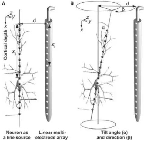
One of the key assumptions of the sCSD method is, that the main axis of the cell is parallel to the electrode. Although, this is roughly possible experimentally, for example when recording from pyramidal neurons the linear probe is inserted perpendicular to the brain surface. Therefore, we wanted to investigate, how much distortion in the result is done when our assumption is not met. As shown in 2.1, we described the position of the cell with the(d)distance of the soma from the electrode and with 2 angles,α marks the angle between being parallel and the main axis of the cell,β shows the rotation around thexaxis.

To see the effect, we created known current source distributions and a certainα,β andd and performed the reconstruction as if the cell was perfectly parallel with the linear probe.

2.3 Development of the skCSD method

The skCSD method aims to provide information about the fine details of the electrophysiological behavior of an observed cell by estimating the membrane current source density distributions. Due to the high temporal and spatial resolution of the multielectrodes used for recording and hence providing the extracellular potentials to the skCSD method, the resolution of the method is belowmsand few tens ofµm. Definitely such a new method must stand must be tested in diverse situations. This goal is challenging in terms of experimental and theoretical methods as well, but the first one we leave to others. As the

(11)

Figure 2.1: Schematic figure about the ideal experimental setup and when the cell is tilted and rotated. In the ideal case, the main axis of the cell is parallel and each current sources marked by grey dots are d distance away from the electrodes. When the cell is tilted withα and rotated withβ, d marks the distance of the soma from the nearest electrode.

(12)

basis of the mathematical model we rely on the already existing current source density method and build on these our novel ideas and approaches.

The first milestone was to create the theoretical relationship between the continuous membrane CSD distribution and the finite sampled extracellular potentials. Second, validation of the method is vital, for this reason simulated data was generated. In this way the ground truth is known and we could construct various scenarios from simple to complex ones. As a third milestone, we applied the method on real experimental data.

(13)

3 Methods

The content of this chapter is a guide and description of the method, the techniques and the experimental data used in the following chapter.

3.1 Overview of current source density reconstruction meth- ods

The methods described here are all used with the exception of the inverse CSD for deriving our results, which was included here for the completeness of the list.

3.1.1 Traditional CSD

For the reader’s convenience, here we briefly present the basic ideas behind the traditional and recent approaches to reconstruction of current source density (CSD analysis).

The relation between current sources in the tissue and the recorded potentials is given by the Poisson equation

C=−∇(σ∇V), (3.1)

whereCstands for CSD andV for the potential. While this can be studied numerically for nontrivial conductivity profiles [Torbjrn et al. 2016], here we shall mostly assume a constant and homogeneous conductivity tensor,σ. In that case, the above equation simplifies toC=−σ∆V and can be solved forCgiven the potential in the whole space.

On the other hand, given the potential in the whole space, the potential is given by V(x) = 1

4πσ Z

d³x^′ C(x^′)

|x−x^′|. (3.2)

Thetraditional CSD methodrelies on the discretised, 1 dimensional (z) form of the Poisson-equation

C(z) =−σd²V(z)

dz² (3.3)

Walter Pitts observed that having recordings on a regular grid of electrodes we can estimate CSD by taking numerical second derivative of the potential [Pitts 1952], we call this approachtraditional CSD method. Pitt’s idea gained popularity only after Nicholson and Freeman popularized its use for laminar recordings [Nicholson et al. 1975] in the cortex. Considering the assumptions below:

(14)

• quasistatic approximation of Maxwell’s equations

• linear extracellular medium

• ohmic (resistive) medium

the following approximation can be derived:

C(zj) =−σV(zj+h)−2V(zj) +V(zj−h)

h² , (3.4)

wherez_j is the position of the j^th electrode andhis the inter-electrode distance. As this is based on the finite differences solution and the precision is of orderO(h²), in higher dimension the error of the approximation is even bigger. Furthermore, the CSD method relies on several other

3.1.2 Inverse CSD (iCSD)

To overcome limitations of the traditional approach, such as difficulty of handling the data at the boundary and hidden assumptions about the dimensions we do not probe, Pettersen et al. proposed a model-based inverse CSD method [Pettersen et al. 2006].

Initially proposed in 1D, the method was later generalized to other dimensionalities [Łeski et al. 2007; Łeski et al. 2011]. Given a set of recordingsV₁, . . . ,VN at regularly placed electrodes atx₁, . . . ,xN this method assumes a model of CSD parameterized with CSD values at the measurement points,C(x) =∑^N_k=1C_kf_k(x), where f_k(x)are functions taking 1 at x_k, 0 at other measurement points, with the values at other points defined by the specific variant of the method, for example, spline interpolated in spline iCSD [“Current Source Density (CSD) Analysis”]. Assuming the modelC(x)one computes the potential at the electrode positions obtaining a relation between the model parameters,C_k, and the measured potential,V_k, which can be inverted leading to an estimate of the CSD in the region of interest.

3.1.3 Volume CSD (vCSD)

The method Riera et al. 2014 estimates the currents as point sources distributed evenly along a 3-dimensional grid. The current distribution (C) is calculated from the extracellular potential (V) by the following formula:

C= (G^′G+λL^′L)⁻¹G^′V (3.5)

(15)

where G is the discrete generalized Green’s function matrix, L is the discrete spatial Laplacian operator,λ is the regularization parameter. In this case, thei j-th element of G takes the value of:

G_{i j}= 1

4πd_{i j}, (3.6)

wheredi j is the distance between the i-th electrode and j-th current source. According to our experience, this method may give a better reconstruction of the current source distribution compared to the traditional CSD method, but the result highly depends on the regularization parameter and the calculation is computationally very demanding. We used a regular grid with 50µminterelectrode distance covering the whole volume of recording.

3.1.4 Kernel CSD (kCSD)

The kernel Current Source Density method [Potworowski et al. 2012] can be considered a generalization of the inverse CSD. It is a non-parametric method which allows reconstructions from arbitrarily placed electrodes and facilitates dealing with the noise. Conceptually, the method proceeds in two steps. First, one does kernel interpolation of the measured potentials. Next, one applies a “cross-kernel” to shift the interpolated potential from the potential to the CSD space. In 3D space, in a homogeneous and isotropic conductivity field, this amounts to applying the Laplacian to the interpolated potential, Eq. (3.1). To handle all cases in a general way, including data of lower dimensionality or with non-trivial conductivity, we construct the interpolating kernel and cross-kernel from a collection of basis functions. The idea is to consider current source density in the form of a linear combination of basis sourcesebj(x), for example Gaussians,

C(x) =

M

∑

j=1

ajebj(x), (3.7)

where the number of basis sources M ≫N, the number of electrodes, and a_j are the weights with which the basis sources are combined into the model CSD. Letbj(x)be the contribution to the extracellular potential fromebj(x), which in 3D is

b_j(x,y,z) =Aeb_j(x,y,z) = 1 4πσ

Z dx^′

Z dy^′

Z

dz^′ eb_j(x^′,y^′,z^′)

p(x−x^′)²+ (y−y^′)²+ (z−z^′)², (3.8) but in 1D or 2D we would need to take into account the directions we do not control in the experiment (for example, along the slice thickness for a slice placed on a 2D MEA). There exists a linear operatorA :space of sources→space of potentials, that the potential will

(16)

have a form

V(x) =AC(x) =

M

∑

i=1

aibi(x). (3.9)

Since we cannot estimateMcoefficientsa_jfromNmeasurements forN<M, we construct a kernel for interpolation of the potential,

K(x,x^′) =

M

∑

i=1

b_i(x)bi(x^′). (3.10)

Then, any potential fieldV(x)spanned byb_i(x)can be written as V(x) =

L

∑

l=1

β_lK(x_l,x), (3.11)

for someL,x_l, andβ_l, but it minimizes the regularized prediction error

N

∑

k=1

(V(xk)−Vk)²+λ

L

∑

l=1

β_l², (3.12)

when L=N. Here, x_k are the positions of the electrodes, V_k are the corresponding measurements,λ is the regularization constant. The minimizing solution is obtained for

β = (K+λI)⁻¹·V. (3.13)

whereVis the vector of the measurementsV_k, andK_jk=K(xj,x_k).

To estimate CSD we introduce a cross-kernel K(e x,x^′) =

M

∑

j=1

b_j(x)eb_j(x^′). (3.14) If we define

e

K^T(x):= [K(e x₁,x), . . . ,K(e x_N,x)], then the estimated CSD takes form of

C^∗(x) =Ke^T(x)·(K+λI))⁻¹·V, (3.15) whereλ is the regularization parameter andIthe identity matrix; see [Potworowski et al.

2012] for derivation and discussion.

(17)

3.1.5 Spike CSD (sCSD)

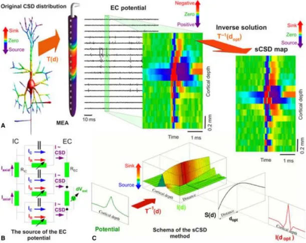
The Spike CSD [Somogyv´ari et al. 2012] is the forerunner of the method presented here, as it aims to estimate the current source distribution of single neurons with unknown morphology. The sCSD method provides an estimation of the cell-electrode distance and uses a simplified model of the shape of the neuron to reach this. Separating potential patterns generated by different neurons is critical and it is obtained by clustering extracellular fingerprints of action potentials which are different for every neuron. The limitation of sCSD is the assumed simplified morphology of the model and low spatial resolution.

Despite that, even with this simplified model, it was possible to demonstrate for the first time the EC observability of backpropagating action potentials in the basal dendrites of cortical neurons, the forward propagation preceding the action potential on the dendritic tree and the signs of the Ranvier-nodes [Somogyv´ari et al. 2012].

Theoretical formalism In this approach, the current source density distribution of a cell will be modelled as N point sources along a line, which is parallel with the linear probe, which has N recording sites. In this case the connection between the recorded potentials and the point sources can be describes by the discrete form of the Poisson equation can be written as:

V_i(ri) = 1 4πσ

N

∑

j=1

C_j

|ri−pj|, (3.16)

wherer_iis the position of thei-th electrode and p_j of the j-th current source. It can be written also in a matrix formalism:

V=TC (3.17)

WhereT is the transfer matrix. In order to get the current sources:

C=T⁻¹V (3.18)

Where the elements ofT can be calculated as T_{i j} = 1

4πσdi j

(3.19) , whered_{i j} is the distance of thei-th electrode from the j-th current source. Asd_{i j} is not known, a measure is introduced (Figure 3.1.C) based on apriori knowledge in order to get an estimation. This method focuses on estimating the CSD around the time of the spike, the expected CSD pattern can be used for creating a metric for estimating the correct distance. As at the emission of an action potential positive ions flow into and negative ions out from the soma, int the neighboring part of the cell membrane the opposite happens,

(18)

there is a balancing counter current. In cases of few tens of micrometers this should result in a sCSD pattern with a:

• peak at the level of the soma

• small, inverse signed values neighboring sources.

The following measureScaptures this behavior:

S(d) =∑I_−s(d)− |Is|

I_s(d) (3.20)

wheredis the hypothetical cell to electrode distance for the reconstruction,Isthe reconstructed current source for the soma and∑I−s is the sum of all the other current sources at the peak of the spike. The maximum value of this function will give the best assumption for the cell-to-electrode distance. Once the most appropriate distance is identified, it is straightforward to solve the Poisson equation for N point sources and N electrodes. The schematic description and main steps of the method are presented on Figure 3.1.

(19)

Figure 3.1: Schematic picture of the basic steps and assumptions of the sCSD method.

A. Assumed experimental setup. The linear probe is parallel to the main axis of the neuron.

We model the current source distribution of the cell showed by the colorscale as N point current sources along the main axis of the cell. The exracellular potential is then recorded by N electrodes. On the measured extracellular potentials we take the potential with a certain time-window around a spike and on all channels, this is shown as spatio-temporal colormap of the extracellular potential. For a better signal-to-noise ratio we used the spike triggered averages. Then by using an estimated cell-to-electrode distance, the sCSD is calculated by using a transfer matrix. The resulting sCSD is also shown as a colormap, on which red color indicates current sinks, value colors current sources. B. Schematic figure shows the connection between currents and the extracellular potential. The CSD is composed of resistive and capacitive membrane currents and the extracellular potential at a point in space is the superposition of the potentials related to the CSD current sources. C.

To get an estimation for the cell-to-electrode distance, a measure is introduced which finds the biologically most relevant distance based on the sCSD pattern at the spike. As the first step, the sCSD distributions are calculated for 1,2... 200µm distances at the time of the spike. Then by using a measure, the peakiest spatial distribution is used, as by the time of the spike we expect a large current sink at the soma and small sources in the neighboring

points.

(20)

3.1.6 Technical tools for the validation of the CSD methods

3.1.6.1 Construction of ground truth data

To validate the method we used simulated data which allows us to consider arbitrary cell- electrode setups and test various current patterns. The LFPy package [Lind´en et al. 2014]

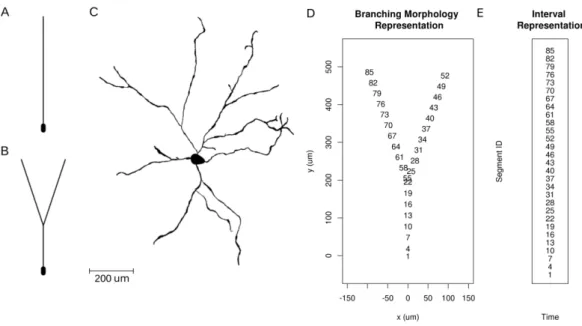
was used to simulate the extracellular potential at arbitrarily placed virtual electrodes. We assumed the.swcmorphology description format Cannon et al. 1998 and the sections were further divided to segments. The coordinates of every segment’s ends were used to find the connections. Once the connection matrix was calculated, we used the Chinese postman algorithm to obtain the morphology loop. We calculated the potential using neuron models with various morphologies shown in Fig. 3.2 and different input distributions, assuming one- and two-dimensional multielectrode arrays. We used toy models to better understand and characterize the method as well as a biologically realistic neuron model to estimate performance of skCSD in an experimentally realistic scenario.

Figure 3.2: Neuron morphologies used for simulation of ground truth data. A. Ball- and-stick neuron. B. Y-shaped neuron. C. Ganglion cell. D. Branching morphology representation of the Y-shaped neuron. The numbers show the segment ID of the morphology.

E. Interval representation of the Y-shaped neuron. The dendrites of the neuron are aligned along a line.

The simplest setup we used was a ball-and-stick neuron recorded with a laminar probe.

Various artificial CSD patterns and also biologically more realistic CSD distributions served as test distributions in order to quantify the spatial resolution and reconstruction errors. To generate the ground truth data we simulated a 500µm long linear cell model of 52 segments in LFPy. The diameter of the two segments representing the soma was 20µm,

(21)

while the other segments were 4µm wide. 100 synaptic excitation events were distributed randomly along this morphology in order to imitate a biologically realistic scenario.

To test the effect of branching on the results, a simple Y-shaped morphology was used (Fig. 3.2B). The synapses were placed at segments 33 and 62 on different branches close to the branching point. The first was stimulated at 5, 45, 60 ms, the other at 5, 25, 60 ms after the onset of the simulation. The idea here was to consider the inputs stimulated together and separately. The times of activation were randomly selected in such a way as to leave enough time for the membrane activity to settle down. This can be viewed as extreme cases of correlated and uncorrelated events. Note that the skCSD reconstruction is not affected directly by the temporal correlation of the synaptic inputs. Just like any CSD estimation method, skCSD is applied to the potentials recorded at a given point in time. Of course, it is affected indirectly, in the sense that slower or faster oscillating inputs lead to different spatial patterns due to filtering effects of the dendritic membrane: fast oscillations induce short dipoles, slow oscillations allow the current to spread along the cell leading to stronger dipoles [Lind´en et al. 2010]. We address these effects indirectly in Fig. 4.10.

As a realistic example we used a mouse retinal ganglion cell morphology Kong et al.

2005 from NeuroMorpho.Org Ascoli 2006. In the simulations 608 segments were used.

100 synaptic excitation events were distributed randomly along this morphology within the first 400 ms of the simulation. The cell was also driven with an oscillatory current. In the dendrites, only passive ion channels were used.

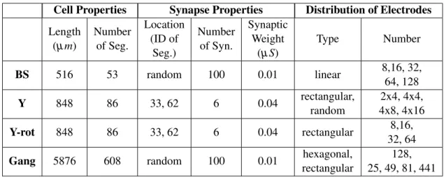
Parameters of the simulations. We simulated three different model morphologies: ball- and-stick (BS), Y-shaped (Y), and a ganglion cell (Gang). The Y-shaped neuron was considered in two situations, when it was parallel (Y) or orthogonal (Y-rot) to the MEA plane. The extracellular potential was computed at multiple points modeling different experimentally viable recording configurations (cell and setup). All combinations used are summarized in Table 3.1. The parameters describing the neuron membrane physiology are given in Table 3.2. The length of the simulation was 70 s in case of the ball-and-stick and Y-shaped neurons, and 850 s for the ganglion cell model.

Parameters of synapses. In most simulations we modeled synaptic activity. We used synapses with discontinuous change in conductance at an event followed by an exponential decay with time constantτ (ExpSyn model as implemented in the NEURON simulator).

When simulating the Y-shaped neuron we placed two synapses with the following parameters: reversal potential: 0 mV , synaptic time constant: 2 ms, synaptic weight: 0.04µS.

The synapses were placed at segments 33 and 62 (See Fig. 3.2 and 4.12). When simulating

(22)

Table 3.1: Main parameters of the simulated cells and setups.

Cell Properties Synapse Properties Distribution of Electrodes Length

(µm)

Number of Seg.

Location (ID of

Seg.)

Number of Syn.

Synaptic Weight

(µS)

Type Number

BS 516 53 random 100 0.01 linear 8,16, 32,

64, 128

Y 848 86 33, 62 6 0.04 rectangular,

random

2x4, 4x4, 4x8, 4x16

Y-rot 848 86 33, 62 6 0.04 rectangular 8,16,

32, 64

Gang 5876 608 random 100 0.01 hexagonal,

rectangular

128, 25, 49, 81, 441

Table 3.2: Biophysical parameters characterizing the simulated cell models.

Quantity Value Unit

Initial potential -65 mV

Axial Resistance 123 Ωcm

Membrane resistivity 30000 Ωcm²

Membrane capacitance 1 µF/cm²

Passive mechanism reversal potential -65 mV

the other models (ball-and-stick and ganglion cell) we used the same type of synapse, however, the synaptic weights were a quarter of the above (0.01µS) since they were more numerous (Table 3.1).

3.1.6.2 Measuring the Quality of Reconstruction

To validate the skCSD method we need to consider two situations. When we know the ground truth — the actual distribution of sources which generated the measured potentials

— we can compare the reconstruction with it. This is available directly only in simulations.

In that case we can measure the prediction error between the reconstruction and the original.

However, the skCSD method by its nature gives smooth results. This is a consequence of kernel interpolation of the potential which occurs in the first step of the method. The same phenomenon occurs in regular CSD estimation [“Current Source Density (CSD) Analysis”]. Thus, we can never recover the original CSD distribution but only a coarse- grained approximation. This is not a significant problem as the coarse-grained CSD should have equivalent physiological consequence. However, to compare the reconstructed density with the ground-truth, which is typically very irregular in consequence of multiple synaptic activation, we always smoothed the ground truth CSD with a Gaussian kernel. The width

(23)

of the kernel was 15µmfor ball-and-stick model, while for the Y-shaped and ganglion cell models we used 30µm.

Thus, whenever ground truth was known, we computed L1 norm of the difference between the reconstructionC^∗and smoothed ground truthCnormalized by the L1 norm of C:

ε_L1=

∑

segments,time|C−C^∗|

∑

segments,time|C| . (3.21)

When analyzing experimental data we only have access to the noisy measurements and cannot apply the above strategy directly. Thus we consider two strategies. One is to use cross-validation error (CV). In leave-one-out cross-validation [Potworowski et al. 2012]

we estimate CSD from all the measurements but one and compare estimated prediction with actual measurement on the removed electrode. Repeating this procedure for all the electrodes gives us a measure of prediction quality for a given set of parameters for this specific dataset. Scanning over some parameter range we identify optimal parameters as those giving minimum error. They are further used to analyze the complete data. The advantage of using cross-validation error is that it does not require the knowledge of the ground truth current source density distribution and can still provide an estimation about the performance of the skCSD method. As this algorithm is quadratic in the number of electrodes, for large arrays one might prefer to use the leave-p-out cross-validation instead.

When we test how the quality of the reconstruction changes with the number of electrodes we use CV error normalized by the number of electrodes which can then be compared between different setups.

The other strategy we use and recommend in the experimental context. The idea is to simulate different current source distributions, either placing specific distribution by hand or by modeling activity of the cell assuming passive membrane and random or specific synaptic activation, both of which are relatively inexpensive both in computational time and coding complexity. This reduces the problem to the modeling case. We can use thus generated data (CSD and potentials) scanning for optimal reconstruction parameters to be used in analysis of actual experimental data from the setup.

To handle the effects of noise one should study its properties on electrodes, e.g., assuming white measurement noise identify its variance, then tune the regularization parameterλ on simulated sets with comparable simulated noise added.

3.1.6.3 Parameter selection

To apply the skCSD method we need to decide upon the number of basis functions, set their width (R), and choose the regularization parameterλ. In this work the number of

(24)

basis function was set to 512 for all cases, which is at least twice the number of electrodes used. This is usually not a limitation, the more the better. For the basis width (Eq. (4.5)) we took the following values: 8, 16, 32, 64, 128µm. Selection of the regularization parameter is not trivial [Potworowski et al. 2012;Discrete Inverse Problems]. Here, we tested the effect of the regularization parameter taking values of 0.00001, 0.0001, 0.001, 0.01, 0.1 The optimal parameters were identified by the lowest value of reconstruction error.

3.1.6.4 Visual representation of CSD on the morphology

To visualize the distribution of current sources and other quantities along a neuron morphology we use two representations of the cell:

1. Interval representation: we stack all the compartments consecutively along the y- axis so that the part of the dendrite stemming from the soma is shown first, followed by one branch, followed by the other. The order of the branches in the stack is taken from the morphology loop to make these representations consistent. Thex-axis either shows different time instants of the simulations or various distribution patterns.

2. Branching morphology representation: in this case a two-dimensional projection of the cell is shown which is colored according to the amplitudes of the membrane current source densities at a time instant. To visually enhance the current events, gray circles proportional to the amplitude of CSD at a point are placed centered at the point to facilitate comprehension.

3.2 Recording and pre-processing the experimental data

As a proof-of-concept of the skCSD method (Section 4.3), its performance was tested on experimental data. In this section the methods of the recording and data pre-processing is to be found.

In vitro experiment One male Wistar rat (300g) was used for the slice preparation procedure. The in vitro experiment was performed according to the EC Council Directive of November 24, 1986 (86/89/EEC) and all procedures were reviewed and approved by the local ethical committee and the Hungarian Central Government Office (license number: PEI/001/695-9/2015). The animal was anesthetized with isoflurane (0.2 ml/100g).

Horizontal hippocampal slices of 500 m thickness were cut with a vibratome (VT1200s;

Leica, Nussloch, Germany). We followed our experimental procedures developed for human in vitro recordings [Kerekes et al. 2014], adapted to rodent tissue. Briefly, slices were transferred to a dual superfusion chamber perfused with artificial cerebrospinal

(25)

fluid. Intracellular patch-clamp recordings, cell filling, visualization and three-dimensional reconstruction of the filled cell was performed as described in [Kerekes et al. 2014]. For the extracellular local field potential recordings, we used a 16-channel linear multielectrode (A16x1-2mm-50-177-A16, Neuronexus Technologies, Ann Arbor, MI, USA), with an INTAN RHD2000 FPGA-based acquisition system (InTan Technologies, Los Angeles, CA, USA). The system was connected to a laptop via USB 2.0. Wideband signals (0.1—7500 Hz) were recorded with a sampling frequency of 20 kHz and with 16-bit resolution. The recorded neuron was held by a constant−40 nA current injection.

Data pre-processing 154 spikes were detected on the 180s long intra-cellular recording by 0mV upward threshold crossing. A 5ms wide time windows were cut around the moments of each spikes on each channels of the extra-cellular (EC) potential recordings and averaged, to access the fine details of the EC spatio-temporal potential pattern which accompanied the firing of the recorded neuron on all channels. Two channels were broken (2, 5), however, as the skCSD method allows retrieving CSD maps from arbitrarily distributed contacts, this has not prevented the analysis; the broken channels were excluded from further consideration. The averaged spatio-temporal potential maps were high-pass filtered by subtracting a moving window average with 100 ms width. This filtering, together with the spike triggered averaging procedure, ensured that the resulted EC potential map contains only the contribution from the actually recorded cell. The price we paid was filtering out EC signals of the spontaneous repetitive sharp-wave like activity of the slice which was correlated by the firing of the recorded neuron and thus the presumptive synaptic inputs of the recorded neuron as well. An additional temporal smoothing by a moving average with 0.15 ms window was used to reduce the effect of noise.

(26)

4 Results

4.1 Results related to the existence of monopole sources

In order to check our hypothesis, the following steps were carried out:

1. Simulate extracellular potential of a firing cell on a 3D electrode grid and take various interelctrode distances, in order to see the change in the spatial sampling, for the same volume

2. Use tCSD and vCSD methods to calculate the current source distributions source distribution

3. Calculate the monopole, dipole and quadrupole moments for both tCSD and vCSD:

4.1.1 Description of the simulations

To validate the method we used simulated data which allows us to consider arbitrary cell- electrode setups and test various current patterns. The LFPy package [Lind´en et al. 2014]

was used to simulate the extracellular potential at arbitrarily placed virtual electrodes.

Y-shaped neuron In this investigation we started with a simple cell model, very similar to the one described in Paragraph 4.3.2.2, with the only difference, that the size of the cell was scaled up, but other parameters regarding the electrophysiological properties remained unchanged. The soma of the cell was placed to the (0,-800,0) position. The dimensions of the electrode grid was 1200µmx 800µmx 1400µmwith interelectrode distances varying between 50, 100, 200µm. A 2 dimensional projection of the setup is show on Figure 4.1.k, where the black circles represent the densest electrode grid setup and the shape of the cell is also shown.

Pyramidal neuron The electrodes were distributed in the same volume of 1200 µm x 800µmx 1400 µm, in the 3 different basic setups the interelectrode distances in all directions were 50, 100, 200µm. In this case a CA3 pyramidal neuron [Ishizuka et al. 1995]

was selected from the NeuroMorpho database for the electrophyisiological simulations.

The simulation lasted for 70 ms, active channels were located only on the soma, passive channels as well as synapses were similarly distributed on the apical and basal dendrites.

TheExpSynsynapse model was used with time constantτ =2 ms, synaptic weight: 0.01 µS, reversal potential: 0 mV. During the time of the simulation altogether 1000 synaptic

(27)

inputs arrived to 100 synapses, these were distributed randomly along the cell. More parameters of the simulation are to be found in Table 3.2.

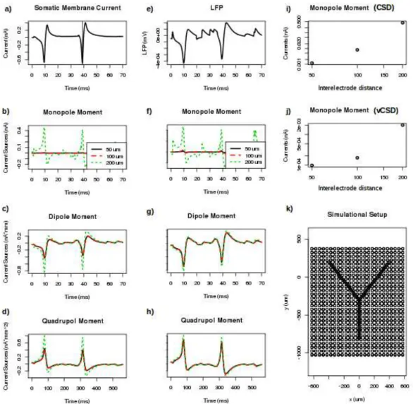
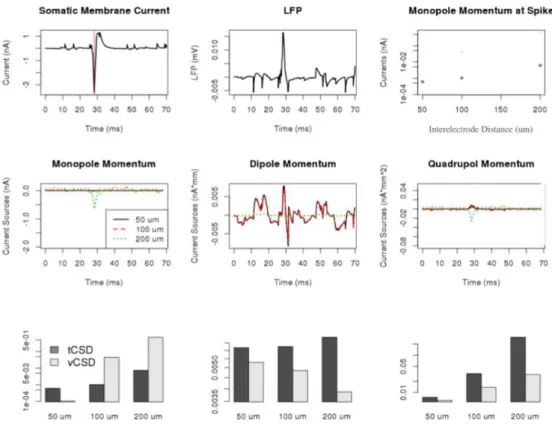
Figure 4.1: tCSD and vCSD reconstruction of simulated extracellular potential. a) So- matic membrane current. The vertical line shows the time instant, when the current moments were compared on part f). b) CSD monopole current moments, where the colour indicate various interelectrode distances. c) CSD dipole moments. d) CSD quadrupol moments.

e) Extracellular potential measured by the electrode placed nearest to the soma. f) vCSD monopole current moments, where the colours indicate various interelectrode distances. g) vCSD dipole moments. h) vCSD quadrupol moments. i) CSD monopole moments at the peak of spike as a function of the interelectrode distance. j) vCSD monopole moments at the peak of spike as a function of the interelectrode distance. k) Section of the simulational setup, where the circles mark the location of electrodes in case of 50 µm interelectrode

distance and the black shape shows the morphology of the toy neuron.

(28)

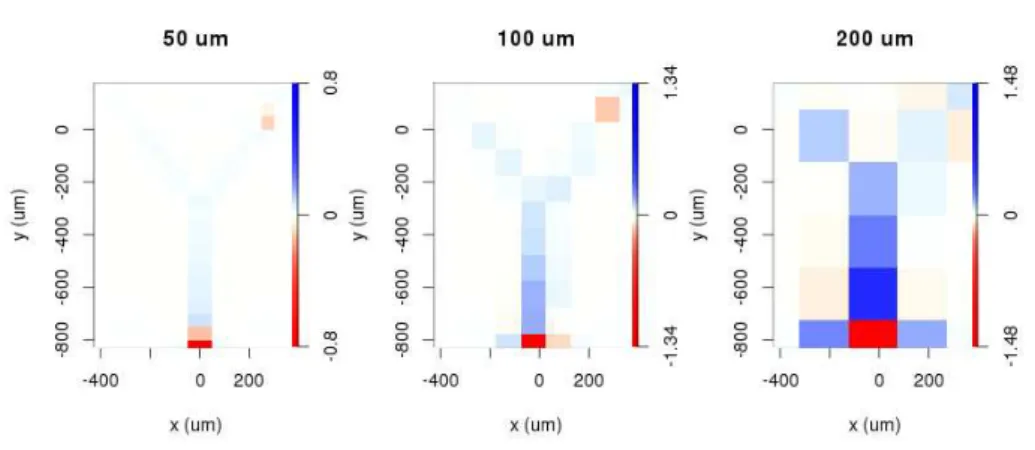
4.1.2 Calculation of current source density distributions

From the extracellular potentials retrieved from the simulation, the tCSD and vCSD can be calculated for each interelectrode distance. The regularization parameter for vCSD had the value ofλ=100. The CSD values on the x-y planes closest to the soma for the Y-shaped cells are shown on Figures 4.2 and 4.3 for 50,100 and 200µminterelectrode distances. Note, that as the vCSD method calculates to CSD values at the electrode grid points and the tCSD method at in between, in case of the same electrode setup used, it was only possible to show the values 25µmapart from each other. Still, the effect of finite spatial sampling is clearly visible, the resolution gets worse and worse with the increase of the interelectode distance, the finite details are lost.

4.1.3 Calculation of the moments

The moments were calculated by using the following equations:

• Monopole moment:

M(t) =

∑

^I(r), ^(4.1)

whereM(t)is the the monopole moment at timetandI(r)is the current in location r.

• Dipole moment:

D_y(t) =

∑

^I(r)(r^y⁻^r⁰^), ^(4.2)

where D_y(t) is the the dipole moment for the y axis at time t and r_y−r₀ is y component of the position of the current source measured from the origo.

• Quadrupole moment:

Q_y(t) =

∑

^I(^r^)(ry−r₀)² (4.3) whereQ_y(t)is the the quadrupole moment for the y axis.

Thereafter in order to get currents (I) from the current source density (C) at a point, each value was multiplied by the volume of the cube with the sides of the interelectode distances in case of tCSD. As in case of VCSD we calculated the current in each point of a grid with 50µmgrid constant, the CSD values were multiplied by 50³µm³.

4.1.4 Revealing the moments

For a more quantitative understanding, we plotted the monopole, dipole quadrupole moments for the 70 ms of the simulations for both vCSD and tCSD together with the

(29)

Figure 4.2: Reconstruction with the traditional CSD method at the plane 25 µm from the plane of the Y-shaped cell. The interelectrode distance is increasing from left to right,

which is inducing a reconstruction error.

Figure 4.3: Reconstruction with the vCSD method at a plane of the Y-shaped cell by using the regularization parameter value 100 in each cases.The reconstruction is distorted

in a different way compared to CSD.

somatic membrane current and measured extracellular potential by the electrode closest to the soma on Figure 4.1. Not surprisingly, the biggest deviation of the moments happens, when there are big changes in the membrane currents and so in the extracellular potential.

When looking at the values of the monopole moment at the peak of the spike on Figure 4.1 i) and j), the tendency for both methods is the same, the better the resolution, the smaller the monopole moment is.

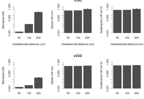
Furthermore as Figure 4.4 highlights, while the other moments are not that effected by the resolution, the apparent monopole moment highly depends on the interelectrode

(30)

distance. In order to get a more robust idea about the appearance of monopole, we considered the average monopole, dipole and quadrupole moment values for three experimental setups, where the electrode grid was shifted by 0, 5, 10, 15, 20, 25µmin case of 50 µm grid constant , 0, 10, 20, 30, 40, 50 in case of 100µmgrid constant, 0, 20, 40, 60, 80, 100 in case of 100µmgrid constant MEAs respectively in the direction ofz.

Figure 4.4: Monopole (left), dipole (middle) and quadrupole moments at the time of spiking activity in case of traditional CSD (above) and vCSD (below) reconstruction in case of the Y-shaped neuron model. The value of monopole moment is highly dependent on the mesh size, a sparse electrode distribution induces bigger ”measured” monopole.

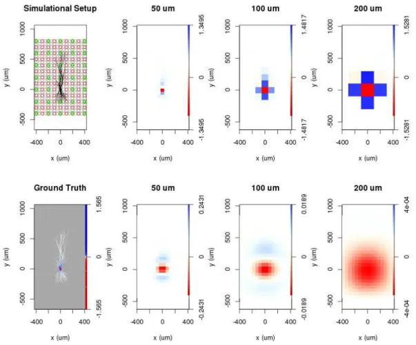
When using a more complicated cell morphology, this conclusion was strengthened.

While the fine electrode grid captures the local changes of membrane current and extracellular potentials during the spike, when using a sparse electrode grids, all details are lost.

The quantitative values presented on Figure 4.6 again support this findings.

(31)

Figure 4.5: Simulational arrangement and visualization of the reconstructed current source distributions estimated by the traditional CSD and vCSD methods in the x-y plane in case of the pyramidal neuron model. The 2 dimensional projections of the morphology of the cell is drawn in black, the position of the recording electrodes are marked by colored circles. According to the various interelectrode-distance, grey, red and green circles correspond to the 50, 100, 200 µm interelectrode-distances. The bottom left figure presents the ground truth membrane current density distribution, red indicates current sinks, blue current sources. The reconstruction with the traditional CSD is shown on the first row, with the vCSD in the second; the 2nd, 3rd and 4th column correspond to the usage of 50, 100, 200µm interelectrode-distances. It is clearly visible that bigger interelectode-distances lead to the distortion of the details of the CSD distribution in case

of both methods.

4.2 Results related to the sensitivity of the sCSD method in case of a tilted cell

The main goal of this section is to present the result related to the investigation of an imperfect cell-electrode setup. There are numerous ways of how this can happen, we limit the studied scenarios to the case, when the cell is tilted with anglesα,β and the distance

(32)

Figure 4.6: Quantitative analysis of CSD reconstructions in case of finite spatial sampling in case of the pyramidal neuron model. The top left and middle figure show the ground truth somatic membrane current and extracellular potential on an electrode close to the soma. The red line indicates the peak of the spike, the monopole-, dipole- and quadrupole moments calculated with the traditional CSD (dark grey dots) and vCSD (light grey dots) at this moment are shown on the top right figure. The detailed temporal course for the vCSD method in case of all interelectrode distances are shown in the second row.

The same quantities are shown in the 3rd row at the the peak of the spike. The standard deviations on the error bars were calculated from averaging the absolute value of moments in the reconstructions in case of shifting electrodes with one-tenth, two-tenth and three-tenth

of the interelectrode distances.

of the soma isd from the electrode as shown in Fig. 2.1.

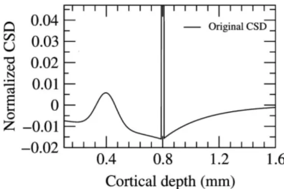
Simulation of ground truth data A ground truth CSD distribution, which is similar to one when firing, was generated as 160 point sources 10µmapart from each other, as shown on Fig. 4.7. The distribution was dominated by a large, point-like sink with an amplitude of 1. The counter currents were symmetric and decayed exponentially as the distance from the soma. A Gaussian-shaped positive current was added to the first branch of. The relative amplitude of these dendritic currents was as small as 1-3 % of the main sink, but in accordance with zero sum requirement, the sums of the currents along the line sources were set to zero in all the three cases.

(33)

Figure 4.7: Ground truth CSD distribution for analyzing the effect of a setup, in case the cell is not completely parallel to the electrode. The amplitudes of the main sinks are normalized to 1, but the graph in the is cut in order to make visible the differences of the

small-amplitude counter currents.

The extracellular potentials were calculated as a superposition of the potential of the point sources,which were distributed on the axis of the cells. The axis of the cell was tilted with anglesα [0^◦,10^◦, ...,60^◦],β[0^◦,45^◦,90^◦], the soma to electrode distance was d [20µm,40µm,60µm]. Tilt towards the electrode within a common plane is denoted by β =0^◦and the tilt perpendicular to the cell–electrode direction is denoted byβ =90^◦. Findings Fig. 4.8 shows how the precision of the CSD reconstruction and the distance estimation depends on the relative angle of cell and the electrode. It was found, that the smaller details of the original CSD diminished on the reconstruction with the increasing tilt, but no spurious sources appeared on the sides of the main sink, which was typical for the tCSD (Fig. 4.8, top row). Parallel, the reconstruction error increased slightly for the sCSD with the increasing tilt, but the RMSE remained lower for sCSD than for tCSD for allα,β and distance combinations (Fig. 4.8, middle row). As the tilt increased, the originally equal distances between different parts of the cell and the line of the electrode became different. This effect is most pronounced in case ofβ =0^◦, thus the reconstruction deteriorates most rapidly in this direction. In these non-parallel cases, we defined the cell–electrode distance as the distance between the soma and the probe, and compared the sCSD distance estimations to it (Fig. 6, bottom row). The distance estimation was relatively insensitive to the tilt forβ =90^◦ and 45^◦ cases, but β =0^◦ results in rapid increase in the distance estimation error with the increasing tilt. Even in this worst case, distance estimation error remained under 20µmup to=20^◦for all examined distances (d

=20, 40, 60µm), thus we concluded, that the distance estimation gives reasonable results up to=20^◦deviation for any case.

(34)

Figure 4.8: Test of CSD sensitivity to the angular deviation between the cell and the electrode. α denotes the deviation from the parallel andβ denotes the direction of the deviation.β=90^◦means, that the deviation is perpendicular to the cell–electrode direction, whileβ =0^◦ marks cell leaning towards the electrode. First row: comparison of sCSD and tCSD reconstruction on examples with increasing leaning fromα =5^◦ toα =20^◦. CSD methods were applied on V patterns calculated from source shown in Fig. 4.7. The small details diminished with the increased leaning. Middle row: leaning dependency of the average CSD reconstruction error in three different leaning directions and distances.

While error increases with the increasing leaning (most rapidly forβ =0^◦), sCSD resulted in smaller error for all cases. The root mean square error (RMSE) values are averages over the 10 different electrode–soma relative positions. Bottom row: leaning dependency of the distance estimation error. Mean errors and the standard error of means are shown.

The distance estimation is relatively insensitive inβ =90^◦andβ =45^◦cases, butβ =0^◦ results in a rapid increase in the distance estimation error. Note the different scale for

β =0^◦.

4.3 Results related to the skCSD Method

4.3.1 Main result regarding the skCSD method

The main result of this work is the introduction of the skCSD method, so we start here with the developement of the theoretical framework. Next, we study the properties of the skCSD reconstruction for three representative morphologies of increasing complexity and

(35)

for different setups.

First, for a ball-and-stick neuron, we study the general quality of reconstruction of fine detail by considering CSD distributions in the form of standing waves of increasing spatial frequency which form the Fourier basis of any possible CSD profile. It is unlikely that standing waves would be naturally observed in a cell, therefore, to better understand how the results for the Fourier space representation relate to a specific distribution which might arise in a physiological situation, we also consider reconstruction of sources for random synaptic activation of the ball-and-stick cell.

Secondly we consider a Y-shaped neuron with a single branching point, we check if skCSD can differentiate between synaptic activation located on the different branches close to the branching point. We also investigate the effects of random distribution of contacts on skCSD reconstruction. Finally, we investigate the possibility of skCSD reconstruction on a realistic model of a ganglion cell placed on a microelectrode array (MEA) as well as the sensitivity of the method to noise.

After establishing and validating skCSD on these fully controlled model datasets, to demonstrate neurophysiological viability, the CSD distribution was reconstructed for a pyramidal cell using the experimental spike-triggered averages of the recorded potentials.

4.3.2 Theoretical framework

The single cell kCSD method (skCSD), which we introduce in this work, is an application of the kCSD framework where we assume that the measured extracellular potential comes mainly from a cell of known morphology and known spatial relation to the MEA. To estimate the CSD in this case we must cover the morphology of the cell with a collection of basis functions. To do this, a one dimensional parametrization of the cell morphology is needed. This could be done independently for each branch of the neuron or globally for the whole cell at once. While the first approach might seem easier, handling of the branching point is non-trivial. Instead, we decided to fit a closed curve on the morphology, which we call themorphology loop(Fig. 4.9). This curve should cover all the segments of the cell, be as short as possible, and be aligned with the morphology. For example, in case of a ball-and-stick neuron, the curve starts at the soma, goes towards the tip of the dendrite, turns back, goes back to the soma, and closes there. One parametersis enough to unambiguously determine a position on this line, although most points on the morphology are mapped to twosparameters. We also need a method to handle the branching points and guide the parametrization so that all the branches will be visited in an optimal way.

This problem is a special case of the Chinese postman problem known from graph theory [Kwan 1962]. Given this information we can distribute the basis functionseb_j(x)along the morphology of the cell (Fig. 4.9).

(36)

In practice, based on the morphology information we define an ordered sequence of all the segments such that the consecutive segments are always physically connected and preference is given to those neighbors which have not been visited yet. The process is continued until all the segments are covered and the last element in the sequence connects to the first element. Note that in the sequence the final segments of the branches are present once, the branching point multiple times and the intermediate ones twice. Then we fit a spline on the coordinates of the segments following the ordered sequence resulting in a morphology loop construction. The CSD basis functions are distributed along this loop uniformly. Any pointx≡(x,y,z)on the morphology can be parameterized withs∈[0,l]

on the loop:

x = f_x(s),

y = f_y(s), (4.4)

z = f_z(s),

wherel is twice the length of all the branches. Consider the following basis functions:

eb_i(s) =e^−(s−sⁱ⁾²^/R² (4.5) wheresiis the location of thei-th basis function on the morphology loop,Rits width.

The contribution to the extracellular potential from a basis sourceeb_i(s)is given by b_i(x,y,z) = 1

4πσ

Z eb_i(s)

p(x−f_x(s))²+ (y−f_y(s))²+ (z−f_z(s))²ds. (4.6)

As in kCSD, for CSD of the form

C(s) =

M

∑

i=1

aiebi(s)

we obtain the extracellular potential as V(x) =

M

∑

i=1

a_ib_i(x). (4.7)

As before, for estimation of potential we use kernel interpolation. Note that in this case the basis functions in the CSD space,eb(s), live on the morphology loop, while the basis functions in the potential space,bi(x), live in the physical 3D space. To determine the current source density distribution along the fitted curve we introduce the following kernel

Dorottya Rita Cserpán THEORETICAL METHODS FOR EXPLORING THE NEUROPHYSIOLOGICAL BEHAVIOR OF SINGLE NEURONS BASED ON EXPERIMENTAL DATA

THEORETICAL METHODS FOR EXPLORING THE NEUROPHYSIOLOGICAL BEHAVIOR OF SINGLE NEURONS BASED ON EXPERIMENTAL

DATA

PhD thesis

Dorottya Rita Cserpán

János Szentágothai Doctoral School of Neurosciences Semmelweis University

Supervisor: Zoltán Somogyvári , Ph.D Official reviewers: Richárd Fiáth , Ph.D

Lajos Kozák, MD, Ph.D

Head of the Complex Exam Committee: Alán Alpár, MD, D.Sc.

Members of the Complex Exam Committee: Árpád Dobolyi, D.Sc.

Emília Madarász, D.Sc.

Budapest

2018

Contents

List of Abbreviations

1 Introduction

1.1 Motivation for studying single neurons with multi- electrode arrays

1.1.1 Levels of functioning

1.1.2 Open questions on the level of single neuron

1.1.3 Multielectrode arrays

1.2 Monopole phenomena

2 Objectives

2.1 Monopole current sources explained

2.2 Sensitivity of sCSD method to the arrangement

2.3 Development of the skCSD method

3 Methods

3.1 Overview of current source density reconstruction meth- ods

3.1.1 Traditional CSD

3.1.2 Inverse CSD (iCSD)

3.1.3 Volume CSD (vCSD)

3.1.4 Kernel CSD (kCSD)

∑

∑

∑

∑

∑

∑

∑

3.1.5 Spike CSD (sCSD)

∑

3.1.6 Technical tools for the validation of the CSD methods

3.2 Recording and pre-processing the experimental data

4 Results

4.1 Results related to the existence of monopole sources

4.1.1 Description of the simulations

4.1.2 Calculation of current source density distributions

4.1.3 Calculation of the moments

∑

∑

∑

4.1.4 Revealing the moments

4.2 Results related to the sensitivity of the sCSD method in case of a tilted cell

4.3 Results related to the skCSD Method

4.3.1 Main result regarding the skCSD method

4.3.2 Theoretical framework

∑

∑